Existence of Quasi-stationary states at the Long Range threshold

Abstract

In this paper the lifetime of quasi-stationary states (QSS) in the $\alpha-$HMF model are investigated at the long range threshold ($\alpha=1$). It is found that QSS exist and have a diverging lifetime $\tau(N)$ with system size which scales as $\mbox{$\tau$(N)$\sim$}\log N$, which contrast to the exhibited power law for $\alpha<1$ and the observed finite lifetime for $\alpha>1$. Another feature of the long range nature of the system beyond the threshold ( $\alpha>1$) namely a phase transition is displayed for $\alpha=1.5$. The definition of a long range system is as well discussed.

1 Introduction

Studying the dynamics of Hamiltonian systems with a large number of degrees of freedom and its connection to equilibrium statistical mechanics has been a long standing problem. The relaxation to statistical equilibrium has been under scrutiny ever since the pioneering work of Fermi and the FPU problemFPU55 . Moreover, since the advent of powerful computers and for specific systems within a class of initial conditions, integrating numerically Hamiltonian dynamics has proven to be competitive in regards to Monte-Carlo schemes for the study of statistical properties (see for instance Leoncini98 ; Torcini99 and references therein). The assumption made is that since the system admits only a few conserved quantities for generic initial conditions, once the dimensions of phase space are large enough, microscopic Hamiltonian chaos should be at play and be sufficiently strong to provide the foundation for the statistical approach within the micro-canonical ensemble. However recent studies have shown that there is an increase of regularity with system size in the microscopic dynamics when considering systems with long range interactions Chavanis-RuffoCCT07 ; Bachelard08 ; Leoncini09b ; Vandenberg10 . Indeed, the statistical and dynamical properties of these systems are still under debate. For instance extensivity is not always provided and discrepancies between canonical and micro-canonical ensembles can be found such as negative specific heats for the latter Dauxois_book2002 ; Campa09 . Moreover, phase transitions for systems embedded in one dimension can be found.

In particular, long range systems often display a slow relaxation to equilibrium. Starting from an initial condition they are in fact trapped in long-lasting out of equilibrium regimes, termed in the literature Quasi Stationary States (QSS) which have distinct macroscopic characteristics, when compared to the equilibrium configuration.

A now paradigmatic model of long range interactions Hamiltonian systems is the Hamiltonian Mean Field (HMF) model Antoni95 , which corresponds to a mean field $XY$-model with a kinetic energy term (rotators). In the limit of infinite system size the HMF model can be described using a Vlasov equation Chavanis2006 ; Campa09 . More recently, stationary states have been constructed using invariant measures of systems composed of uncoupled pendula Leoncini09b , more specifically it was emphasized that the microscopic dynamics in the magnetized stationary state is regular and explicitly known. This observation lead to explain the abundance of regular orbits as revealed in Bachelard08 . These results first obtained for the HMF have been extended for the case when the coupling constant depends on the distance between sites, namely for $\alpha-$HMF model in its long range version ($\alpha<1$)Vandenberg10 . This model was introduced for instance in Anteneodo98 and and displays identical equilibrium features as the HMFTamarit00 ; Campa09 . In fact it was shown that all stationary states of the HMF model are as well stationary states of the $\alpha-$HMF model, that microscopic dynamics is as well regular, at the price of microscopic spatial complexity, which is locally scale invariantVandenberg10 . Before going on we write the governing Hamiltonian of the model:

$$H=\sum_{i=1}^{N}\left[\frac{p_{i}^{2}}{2}+\frac{1}{2\tilde{N}}\sum_{j\neq i}^{N}\frac{1-\cos\left(q_{i}-q_{j}\right)}{\|i-j\|^{\alpha}}\right]\>,$$ (1)

where $q_{i}$ stands for some spin angle located on the lattice site $i,$ and $p_{i}$ is its canonically conjugate momentum. The distance $\|i-j\|$ is actually the shortest distance on the circle of perimeter $N-1$, so that the systems can be isolated and still translational invariant along the lattice. The mean field model is recovered for $\alpha=0$, and for $N$ even, we write

$$\tilde{N}=\left(\frac{2}{N}\right)^{\alpha}+2\sum_{i=1}^{N/2-1}\frac{1}{i{}^{\alpha}}\>,$$ (2)

to insure extensivity. The equations of motions of element $i$ are derived from the Hamiltonian (1):

$$\dot{p_{i}} = -\sin(q_{i})C_{i}+\cos(q_{i})S_{i}=M_{i}\sin(q_{i}-\varphi_{i})\>,$$ (3)

$$\dot{q_{i}} = p_{i}\>,$$ (4)

where

$$C_{i} = \frac{1}{\tilde{N}}\sum_{j\neq i}\frac{\cos q_{j}}{\|i-j\|^{\alpha}}$$ (5)

$$S_{i} = \frac{1}{\tilde{N}}\sum_{j\neq i}\frac{\sin q_{j}}{\|i-j\|^{\alpha}}\>.$$ (6)

$C_{i}$ and $S_{i}$ identify the two components of a magnetization per site, with modulus $M_{i}=\sqrt{C_{i}^{2}+S_{i}^{2}}$ , and phase $\varphi_{i}=\arctan(S_{i}/C_{i})$. For large $N$ , and assuming $0<\alpha<1$, we have

$$\tilde{N}\approx\frac{2}{1-\alpha}(N/2)^{1-\alpha}\>.$$ (7)

We then can use (7) in Eq.(5) and, make the $N\rightarrow\infty$ limit while introducing the continuous variables $x=i/N$ and $y=j/N$ to arrive at

$$C(x)=\frac{1-\alpha}{2^{\alpha}}\int_{-1/2}^{1/2}\frac{\cos\left(q(y)\right)}{\|x-y\|^{\alpha}}dy\>,$$ (8)

where $\|x-y\|$ represents the minimal distance on a circle of perimeter one. We can recognize the fractional integral $I^{1-\alpha}$and consequently write

$$C(x)=\frac{1-\alpha}{2^{\alpha}}\Gamma(1-\alpha)I^{1-\alpha}\left(\cos q(x)\right)\>.$$ (9)

In this large size limit, the $\alpha-$HMF dynamics implies studying the evolution of the scalar fields $q(x,t)$ and $p(x,t)$ which are ruled by the fractional (non-local) partial differential equations

$$\frac{\partial q}{\partial t} = p(x,t)$$

$$\frac{\partial p}{\partial t} = \frac{\mu}{2^{\alpha}}\Gamma(\mu)\left(-\sin(q)I^{\mu}\left(\cos q\right)+\cos(q)I^{\mu}\left(\sin q\right)\right)\>.$$

where $\mu=1-\alpha$. It has then been shown in Vandenberg10 that stationary states are solutions of

$${\mathcal{D}}^{\alpha}\cos q=\frac{d^{\alpha}\cos q}{dx^{\alpha}}=0\>.$$ (10)

where the operator $D^{\alpha}$ stands for the fractional derivative, and that actually this property was shared with non stationary QSS’s. All these results were obtained for the model in its long range version, meaning when $\alpha$ is smaller than one.

2 What happens for $2>\alpha\geq 1$

Figure 1: Magnetization vs energy, for $\alpha=1.5$. A phase transition is displayed with $\epsilon_{c}\approx 0.6$. The transition point seem to be different from the long-range one which is $\epsilon_{c}=0.75$, but the qualitative behavior of curve is the same.

We recall that systems are considered long range when the two body interacting potential $V(r)$ decays at the most as $1/r^{\alpha}$ with $\alpha<d$, where $d$ stands for the dimension of the embedding space. Having only one degree of freedom $d=1$ for the $\alpha-$HMF model. In these regards, considering situations where $1<\alpha<2$ is actually studying short range models, In fact $\tilde{N}$ is finite so there is no need of system size renormalization of the couling constant for $\alpha>1$. However something is peculiar about this lattice model. Indeed when considering the dynamics of a long range system, we would expect the force to be ruled by a $1/r^{\beta}$ decay with $\beta=\alpha+1$, which is not the case for the lattice model for which the decay exponent is unchanged ($\beta=\alpha$). Moreover given the particular importance of the microscopic dynamics and possible ergodicity breaking, one could naturally raise the question if the long range nature of a system is not ruled by the dynamics, which would then imply a system to be long ranged if $\beta<d+1$, which for the $\alpha-$HMF model would imply $\alpha<2$. Most of the previous analysis of the model has been performed for $\alpha<1$, and can not simply be extended to $1<\alpha<2$. A first numerical analysis is therefore necessary.

2.1 Phase transitions

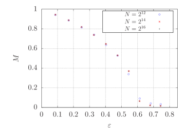
One peculiarity of one dimensional systems, is that there should not bare any phase transition if the interaction is short ranged. A first numerical study of the magnetization versus density of energy is performed for $\alpha=1.5$ in Fig. 1. The numerical integration of the microscopic dynamics is performed using a simplectic scheme, (optimal fifth order seeMcLachlan92 ), a typical time step used is $\delta t=0.05$, and the initial conditions are Gaussian distributed. The fast Fourier transforms are done with the fftw libraries. As can be seen in Fig. 1 a phase transition is displayed at a transition point $\epsilon_{c}\approx 0.6$ which is then different from the universal value obtained for $\alpha<1$ which is $\epsilon_{c}=0.75$. Preliminary results show actually that the critical point depends on the value of $\alpha$ and results seem to show that it approaches $\epsilon=0$ for $\alpha=2$.

Figure 2: Top: Magnetization curve vs time for $\alpha=1.0$, $N=2^{1}8$ and $\epsilon=1.2$. During the QSS the magnetization is oscillating for a time $\tau_{1}$, then it relaxes down to it’s equilibrium value in a time $\tau_{2}$.
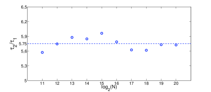
Bottom: $\frac{\tau_{2}}{\tau_{1}}$ for different values of $N$, $\alpha=1$ and $\epsilon=0.6$. The two times are approximately proportional, so the knowledge of $\tau_{1}$ gives a good approximation for $\tau_{2}$. This proportionality is respected for all $\alpha$ values in this paper, even if the proportionality constant may vary.

This existence of a phase transition beyond the “classical” long range threshold in one dimension had already been noticed for the Ising model by Dyson in the sixties, but this feature seems to favor the dynamical definition of what a long range system ought be. However an important feature to assert this new definition would be to find as well quasi-stationary states in this region of $\alpha$’s.

2.2 QSS lifetime

In long range interacting systems, generally, the limit $N\rightarrow\infty$ and $t\rightarrow\infty$ doesn’t commute, so the thermodynamic limit is not unequivocally defined and one may end up in different equilibrium states depending on the order of the previous limits. Physically it’s more feasible to compute the continuous limit before the time limit, so if the lifetime $\tau$ of the QSS diverges with $N$ it becomes the effective real equilibrium of the system, which in general is not obeying Boltzmann’s statistics Chavanis-RuffoCCT07 . We studied how the QSS lifetime scales with the exponent $\alpha$ in the decay parameter of the potential.

First we studied the behavior of the lifetime $\tau$ around the crucial value $\alpha=1$ to better understand the transition between a long range system and a supposedly short range one, but as mentioned in the case of $\alpha$-HMF there are convincing arguments that the requirement for the emergence of long range behavior could be relaxed, and we can expect some long range feature to survive above $\alpha=1$.

Figure 3: Poincaré sections for $\alpha=1$, $\epsilon=1.2$ and $N=2^{20}$. Top refers to the QSS, while bottom represent the relaxation state between $\tau_{1}$ and $\tau_{2}$. It can be easily seen that the second small isle disappear during the relaxation and the phase space becomes symmetric in $q$, thus ending the oscillations of the magnetization.

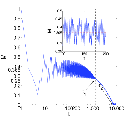
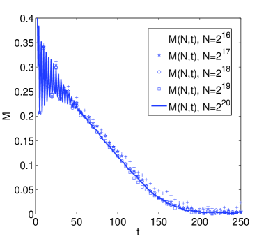
We considered the initial condition already used in Vandenberg10 which was giving rise to a QSS, namely a long lived magnetized state above the critical energy. The initial condition used is all $q_{i}=0$, wile the $p_{i}$’s are Gaussian. To characterize the QSS lifetime we monitor the behavior of the global macroscopic parameter magnetization which can be $M=|\sum_{j}e^{iq_{j}}|$. In Fig. 2 we show the behavior for $\alpha=1$, which is qualitatively representative for the all studied values of $\alpha$ in this paper.

Figure 4: Scaling of $\tau_{1}$ with $N$ for different $\alpha$ values and $\epsilon=1.2$. Top shows the scaling for $\alpha=0.9$; middle refers to $\alpha=1.0$ and shows both $\tau_{1}$ and $\tau_{2}$; while bottom refers to $\alpha=1.1$ . All curves seems to grow at least logarithmically.

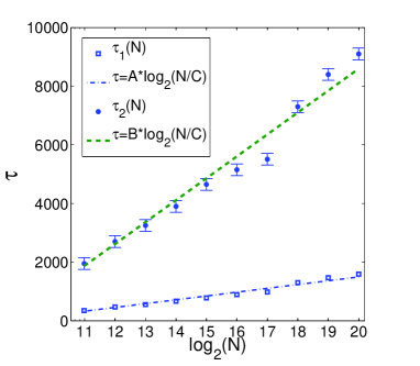
Here a first transition at $t=\tau_{1}$ can be identified until which the system oscillates around an almost constant magnetization value, and beyond which the system starts to relax towards the equilibrium $M=0$ value. A second transition at $t=\tau_{2}$ is as well identified, it corresponds to the time at which the system finally reaches it’s equilibrium state. As can be seen in Fig. 2, we find that these two values are almost linearly proportional for each $\alpha$-value that we took into consideration, so we will refer to the first lifetime $\tau_{1}$ as the lifetime of the QSS, since is an order of magnitude faster to compute and we are interested only in the qualitative form of the scaling law for the lifetimes.

Figure 5: Magnetization curve vs time for $\alpha=1.5$, $\epsilon=1.0$ and increasing $N$ values. The initial oscillation lifetime $\tau_{1}$ is independent of $N$ and the system relaxes to equilibrium in a time which should be constant in the continuous limit.

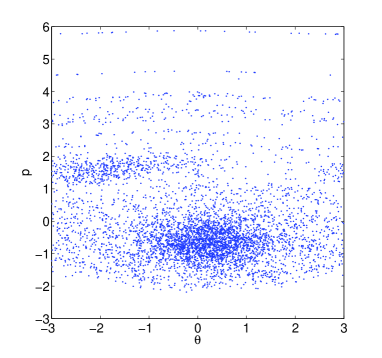
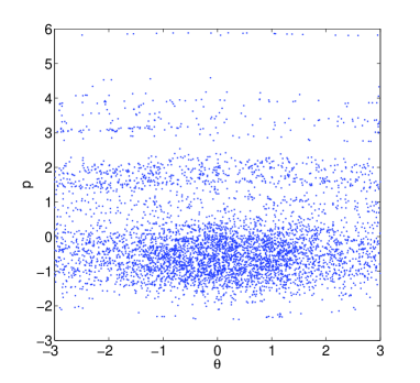
The difference of the two dynamical regimes defined by the above thresholds are better understood when looking at the Poincaré section captured in each of this regimes displayed in Fig. 3. At first the system is forms two distinct islands in the phase space, which start moving around and create the oscillations in the magnetization that characterize the QSS, and then one of the isles disappear during the relaxation period, while the phase space becomes symmetric in $q$ thus ending the oscillations.

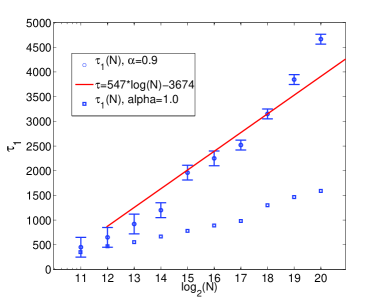
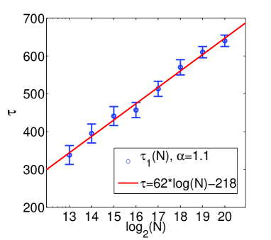
Now we analyze the lifetime of the QSS versus the size of the system around the classical long range threshold $\alpha=1$, if the system is long range it should diverge with $N$. The cases $\alpha=0.9$, $\alpha=1$ and $\alpha=1.1$ are displayed in Fig. 4. We can see that around $\alpha=1$ the scaling of $\tau$ with $N$ approaches a logarithmic curve, meaning that the QSS survive at least until $\alpha=1$ and maybe beyond as it appears as well true for $\alpha=1.1$. However when looking at the data for larger value of $\alpha$, namely $\alpha=1.5$ the scaling of $\tau$ appears to saturate as displayed in Fig. 5, where the magnetization curves obtained for $\alpha=1.5$ appear to all be identical no matter the size of the system. At this value of $\alpha$ there is still a short initial oscillation in $M$ typical of the QSS, but now it’s lifetime seems to be independent of $N$ and finite so the system will reach the equilibrium state in a large enough time. Conversely we may expect that we may actually observe the same feature for $\alpha=1.1$, but that we have not seen yet the saturation in the lifetime as we were not able to simulate systems that would be large enough. In other words, we have as now not enough data to identify if there is a transition value between $1.1<\alpha<1.5$ where the system becomes suddenly short-range dropping the logarithmic law of $\tau_{1}$, or it still saturates at some larger value of $N>2^{20}$ even for $\alpha=1.1$. Preliminary results shows that this saturation becomes quite fast for $\alpha\sim 1.2,1.3$ where even for low values of $N$ it may still be possible to observe a scaling which is sub-logarithmic, but even if it did this would be only relevant for systems with an astronomical scale of constituants.

However even if the QSS lifetime seems to saturate at some point, so that the system dynamics change into a short range one, the phase transition from a magnetized to an homogeneous state, typical of the long range regime, is still present (figure 1). Hence is appears that the dynamical definition may be more relevant for macroscopic features, such as the presence of a QSS (even with a finite lifetime) or a phase transition, while the more classical statistical definition of a long range system corresponds actually to different dynamical behavior of the system and the existence of QSS with diverging lifetimes.

References

- (1) E. Fermi, J. Pasta, and S. Ulam. Los Alamos Reports, (LA-1940), 1955.
- (2) Xavier Leoncini, Alberto Verga, and Stefano Ruffo. Hamiltonian dynamics and the phase transition of the xy model. Phys. Rev. E, 57(6):6377, 1998.
- (3) A. Torcini and M. Antoni. Equilibrium and dynamical properties of two dimensional n-body systems with long range attracting interactions. Phys. Rev. E, 59:2746, 1999.
- (4) P. H. Chavanis, G. De Ninno, D. Fanelli, and S. Ruffo. Out of equilibrium phase transitions in mean-field hamiltonian dynamics. In C. Chandre, X. Leoncini, and G. Zaslavsky, editors, Chaos, Complexity and Transport, pages 3–26, Singapore, 2008. World Scientific.
- (5) R. Bachelard, C. Chandre, D. Fanelli, X. Leoncini, and S. Ruffo. Abundance of regular orbits and out-of-equilibrium phase transitions in the thermodynamic limit for long-range systems. Phys. Rev. Lett., 101(26):260603, 2008.
- (6) X. Leoncini, T. L. Van den Berg, and D. Fanelli. Out of equilibrium solutions in the xy-hamiltonian mean field model. EPL, 86:20002, 2009.
- (7) T. L. Van den Berg, D. Fanelli, and X. Leoncini. Stationary states and fractional dynamics in systems with long range interactions. EPL, 89:50010, 2010.
- (8) T. Dauxois, S. Ruffo, E. Arimondo, and M. Wilkens, editors. Dynamics and Thermodynamics of Systems with Long Range Interactions, volume 602 of Lect. Not. Phys. Springer-Verlag, Berlin, 2002.
- (9) Alessandro Campa, Thierry Dauxois, and Stefano Ruffo. Statistical mechanics and dynamics of solvable models with long-range interactions. Phys. Rep., 480:57–159, 2009.
- (10) M. Antoni and S. Ruffo. Phys. Rev. E, 52:3261, 1995.
- (11) P. H. Chavanis. Lynden-bell and tsallis distributions for the hmf model. Eur. Phys. J. B, 53(4):487–501, 2006.
- (12) Celia Anteneodo and Constantino Tsallis. Breakdown of exponential sensitivity to initial conditions: Role of the range of interactions. Phys. Rev. Lett., 80:5313–5316, 1998.
- (13) Francisco Tamarit and Celia Anteneodo. Rotators with long-range interactions: Connection with the mean-field approximati. Phys. Rev. Lett., 84:208–211, 2000.
- (14) R. I. McLachlan and P. Atela. The accuracy of symplectic integrators. Nonlinearity, 5:541–562, 1992.