Oded Schramm: From Circle Packing to SLE

1 Introduction

When I first met Oded Schramm in January 1991 at the University of California, San Diego, he introduced himself as a “Circle Packer”. This modest description referred to his Ph.D. thesis around the Koebe-Andreev-Thurston theorem and a discrete version of the Riemann mapping theorem, explained below. In a series of highly original papers, some joint with Zhen-Xu He, he created powerful new tools out of thin air, and provided the field with elegant new ideas. At the time of his deadly accident on September 1st, 2008, he was widely considered as one of the most innovative and influential probabilists of his time. Undoubtedly, he is best known for his invention of what is now called the Schramm-Loewner Evolution (SLE), and for his subsequent collaboration with Greg Lawler and Wendelin Werner that led to such celebrated results as a determination of the intersection exponents of two-dimensional Brownian motion and a proof of Mandelbrot’s conjecture about the Hausdorff dimension of the Brownian frontier. But already his previous work bears witness to the brilliance of his mind, and many of his early papers contain both deep and beautifully simple ideas that deserve better knowing.

In this note, I will describe some highlights of his work in circle packings and the Koebe conjecture, as well as on SLE. As Oded has co-authored close to 20 papers related to circle packings and more than 20 papers involving SLE, only a fraction can be discussed in detail here. The transition from circle packing to SLE was through a long sequence of influential papers concerning probability on graphs, many of them written jointly with Itai Benjamini. I will present almost no work from that period (some of these results are described elsewhere in this volume, for instance in Christophe Garban’s article on Noise Sensitivity). In that respect, the title of this note is perhaps misleading.

In order to avoid getting lost in technicalities, arguments will be sketched at best, and often ideas of proofs will be illustrated by analogies only. In an attempt to present the evolution of Oded’s mathematics, I will describe his work in essentially chronological order.

Oded was a truly exceptional person: not only was his clear and innovative way of thinking an inspiration to everyone who knew him, but also his caring, modest and relaxed attitude generated a comfortable atmosphere. As inappropriate as it might be, I have included some personal anecdotes as well as a few quotes from email exchanges with Oded, in order to at least hint at these sides of Oded that are not visible in the published literature.

This note is not meant to be an overview article about circle packings or SLE. My prime concern is to give a somewhat self-contained account of Oded’s contributions. Since SLE has been featured in several excellent articles and even a book, but most of Oded’s work on circle packing is accessible only through his original papers, the first part is a bit more expository and contains more background. The expert in either field will find nothing new, and will find a very incomplete list of references. My apology to everyone whose contribution is either unmentioned or, perhaps even worse, mentioned without proper reference.

Acknowledgement: I would like to thank Mario Bonk, Jose Fernández, Jim Gill, Joan Lind, Don Marshall, Wendelin Werner and Michel Zinsmeister for helpful comments on a first draft. I would also like to thank Andrey Mishchenko for generating Figure 3, and Don Marshall for Figure 6.

2 Circle Packing and the Koebe Conjecture

Oded Schramm was able to create, seemingly without effort, ingenious new ideas and methods. Indeed, he would be more likely to invent a new approach than to search the literature for an existing one. In this way, in addition to proving wonderful new theorems, he rediscovered many known results, often with completely new proofs. We will see many examples throughout this note.

Oded received his Ph.D. in 1990 under William Thurston’s direction at Princeton. His thesis, and the majority of his work until the mid 90’s, was concerned with the fascinating topic of circle packings. Let us begin with some background and a very brief overview of some highlights of this field prior to Oded’s thesis. Other surveys are [Sa] and [Ste2].

2.1 Background

According to the Riemann mapping theorem, every simply connected planar domain, except the plane itself, is conformally equivalent to a disc. The conformal map to the disc is unique, up to postcomposition with an automorphism of the disc (which is a Möbius transformation). The standard proof exhibits the map as a solution of an extremal problem (among all maps of the domain into the disc, maximize the derivative at a given point). The situation is quite different for multiply connected domains, partly due to the lack of a standard target domain. The standard proof can be modified to yield a conformal map onto a parallel slit domain (each complementary component is a horizontal line segment or a point). Koebe showed that every finitely connected domain is conformally equivalent to a circle domain (every boundary component is a circle or a point), in an essentially unique way. No proof similar to the standard proof of the Riemann mapping theorem is known.

Theorem 2.1 ([Ko1]).

For every domain $\Omega\subset{\mathbb{C}}$ with finitely many connected boundary components, there is a conformal map $f$ onto a domain $\Omega^{\prime}\subset{\mathbb{C}}$ all of whose boundary components are circles or points. Both $f$ and $\Omega^{\prime}$ are unique up to a Möbius transformation.

Koebe conjectured (p. 358 of [Ko1]) that the same is true for infinitely connected domains. It later turned out that uniqueness of the circle domain can fail (for instance, it fails whenever the set of point-components of the boundary has positive area, as a simple application of the measurable Riemann mapping theorem shows). But existence of a conformally equivalent circle domain is still open, and is known as Koebe’s conjecture or “Kreisnormierungsproblem”. It motivated a lot of Oded’s research.

There is a close connection between Koebe’s theorem and circle packings. A circle packing $P$ is a collection (finite or infinite) of closed discs $D$ in the two dimensional plane ${\mathbb{C}}$, or in the two dimensional sphere $S^{2}$, with disjoint interiors. Associated with a circle packing is its tangency graph or nerve $G=(V,E)$, whose vertices correspond to the discs, and such that two vertices are joined by an edge if and only if the corresponding discs are tangent. We will only consider packings whose tangency graph is connected.

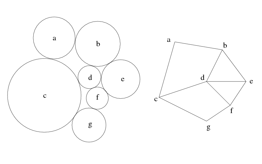
Figure 1: A circle packing and its tangency graph.

Conversely, the Koebe-Andreev-Thurston Circle Packing Theorem guarantees the existence of packings with prescribed combinatorics. Loosely speaking, a planar graph is a graph that can be drawn in the plane so that edges do not cross. Our graphs will not have double edges (two edges with the same endpoints) or loops (an edge whose endpoints coincide).

Theorem 2.2 ([Ko2], [T], [A1]).

For every finite planar graph $G$, there is a circle packing in the plane with nerve $G$. The packing is unique (up to Möbius transformations) if $G$ is a triangulation of $S^{2}$.

See the following sections for the history of this theorem, and sketches of proofs. In particular, in Section 2.3 we will indicate how the Circle Packing Theorem 2.2 can be obtained from the Koebe Theorem 2.1, and conversely that the Koebe theorem can be deduced from the Circle Packing Theorem. Every finite planar graph can be extended (by adding vertices and edges as in Figure 3) to a triangulation, hence packability of triangulations implies packability of finite planar graphs (there are many ways to extend a graph to a triangulation, and uniqueness of the packing is no longer true). The situation is more complicated for infinite graphs. Oded wrote several papers dealing with this case.

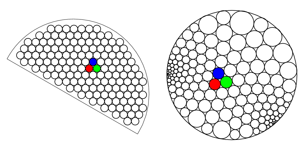
Figure 2: A circle packing approximation to a Riemann map.

Thurston conjectured that circle packings approximate conformal maps, in the following sense: Consider the hexagonal packing $H_{\varepsilon}$ of circles of radius $\varepsilon$ (a portion is visible in Fig. 2 and Fig. 3). Let ${\Omega}\subset{\mathbb{C}}$ be a domain (a connected open set). Approximate ${\Omega}$ from the inside by a circle packing $P_{\varepsilon}$ of circles of ${\Omega}\cap H_{\varepsilon}$, as in Fig. 2 and Fig. 3 (more precisely, take the connected component containing $p$ of the union of those circles whose six neighbors are still contained in ${\Omega}$). Complete the nerve of this packing by adding one vertex for each connected component of the complement to obtain a triangulation of the sphere (there are three new vertices $v_{1},v_{2},v_{3}$ in Fig. 3; the three copies of $v_{3}$ are to be identified). By the Circle Packing Theorem, there is a circle packing $P^{\prime}_{\varepsilon}$ of the sphere with the same tangency graph (Figures 2 and 3 show these packings after stereographic projection from the sphere onto the plane; the circle corresponding to $v_{3}$ was chosen as the upper hemisphere and became the outside of the large circle after projection). Notice that each of the complementary components now corresponds to one (“large”) circle of $P^{\prime}_{\varepsilon}$, and the circles in the boundary of $P_{\varepsilon}$ are tangent to these complementary circles. Now consider the map $f_{\varepsilon}$ that sends the centers of the circles of $P_{\varepsilon}$ to the corresponding centers in $P^{\prime}_{\varepsilon}$, and extend it in a piecewise linear fashion.

Figure 3: A circle packing approximation of a triply connected domain, its nerve, its completion to a triangulation of $S^{2}$, and a combinatorially equivalent circle packing; (a)-(c) are from Oded’s thesis; thanks to Andrey Mishchenko for creating (d)

Rodin and Sullivan proved Thurston’s conjecture that $f_{\varepsilon}$ approximates the Riemann map, if ${\Omega}$ is simply connected (see Fig. 2):

Theorem 2.3.

[RSu] Let ${\Omega}$ be simply connected, $p,q\in{\Omega},$ and $P^{\prime}_{\varepsilon}$ normalized such that the complementary circle is the unit circle, and such that the circle closest to $p$ (resp. $q$) corresponds to a circle containing $0$ (resp. some positive real number). Then the above maps $f_{\varepsilon}$ converge to the conformal map $f:{\Omega}\to{\mathbb{D}}$ that is normalized by $f(p)=0$ and $f(q)>0,$ uniformly on compact subsets of ${\Omega}$ as $\varepsilon\to 0.$

Their proof depends crucially on the non-trivial uniqueness of the hexagonal packing as the only packing in the plane with nerve the triangular lattice. Oded found remarkable improvements and generalizations of this theorem. See Section 2.6 for further discussion.

2.2 Why are Circle Packings interesting?

Despite their intrinsic beauty (see the book [Ste2] for stunning illustrations and an elementary introduction), circle packings are interesting because they provide a canonical and conformally natural way to embed a planar graph into a surface. Thus they have applications to combinatorics (for instance the proof of Miller and Thurston [MT] of the Lipton-Tarjan separator theorem, see e.g. the slides of Oded’s circle packing talk on his memorial webpage), to differential geometry (for instance the construction of minimal surfaces by Bobenko, Hoffmann and Springborn [BHS] and their references), to geometric analysis (for instance, the Bonk-Kleiner [BK] quasisymmetric parametrization of Ahlfors 2-regular LLC topological spheres) to discrete probability theory (for instance, through the work of Benjamini and Schramm on harmonic functions on graphs and recurrence on random planar graphs [BS1],[BS2], [BS3]) and of course to complex analysis (discrete analytic functions, conformal mapping). However, Oded’s work on circle packing did not follow any “main-stream” in conformal geometry or geometric function theory. I believe he continued to work on them just because he liked it. His interest never wavered, and many of his numerous late contributions to Wikipedia were about this topic.

Existence and uniqueness are intimately connected. Nevertheless, for better readability I will discuss them in two separate sections.

2.3 Existence of Packings

Oded applied the highest standards to his proofs and was not satisfied with “ugly” proofs. As we shall see, he found four (!) different new existence proofs for circle packings with prescribed combinatorics. Before discussing them, let us have a glance at previous proofs.

The Circle Packing Theorem was first proved by Koebe [Ko2] in 1936. Koebe’s proof of existence was based on his earlier result that every planar domain ${\Omega}$ with finitely many boundary components, say $m$, can be mapped conformally onto a circle domain. A simple iterative algorithm, due to Koebe, provides an infinite sequence ${\Omega}_{n}$ of domains conformally equivalent to ${\Omega}$ and such that ${\Omega}_{n}$ converges to a circle domain. To obtain ${\Omega}_{n+1}$ from ${\Omega}_{n}$, just apply the Riemann mapping theorem to the simply connected domain (in ${\mathbb{C}}\cup\{\infty\}$) containing ${\Omega}_{n}$ whose boundary corresponds to the $(n\mod m)-$th boundary component of ${\Omega}$. With the conformal equivalence of finitely connected domains and circle domains established, a circle packing realizing a given tangency pattern can be obtained as a limit of circle domains: Just construct a sequence of $m$-connected domains so that the boundary components approach each other according to the given tangency pattern. For instance, if the graph $G=(V,E)$ is embedded in the plane by specifying simple curves $\gamma_{e}:[0,1]\to S^{2}$, $e\in E,$ then the complement $\Omega_{\varepsilon}$ of the set

$$\bigcup_{e\in E}\gamma_{e}[0,1/2-\varepsilon]\cup\bigcup_{e\in E}\gamma_{e}[1/2+\varepsilon,1]$$

is such an approximation. It is not hard to show that the (suitably normalized) conformally equivalent circle domains $\Omega^{\prime}_{\varepsilon}$ converge to the desired circle packing when $\varepsilon\to 0.$

Koebe’s theorem was nearly forgotten. In the late 1970’s, Thurston rediscovered the circle packing theorem as an interpretation of a result of Andreev [A1], [A2] on convex polyhedra in hyperbolic space, and obtained uniqueness from Mostow’s rigidity theorem. He suggested an algorithm to compute a circle packing (see [RSu]) and conjectured Theorem 2.3, which started the field of circle packing. Convergence of Thurston’s algorithm was proved in [dV1]. Other existence proofs are based on a Perron family construction (see [Ste2]) and on a variational principle [dV2].

Oded’s thesis [S1] was chiefly concerned with a generalization of the existence theorem to packings with prescribed convex shapes instead of discs, and to applications. A consequence ([S1], Proposition 8.1) of his “Monster packing theorem” is, roughly speaking, that the circle packing theorem still holds if discs are replaced by smooth convex sets.

Theorem 2.4.

([S1], Proposition 8.1) For every triangulation $G=(V,E)$ of the sphere, every $a\in V$, every choice of smooth strictly convex sets $D_{v}$ for $v\in V\setminus\{a\},$ and every smooth simple closed curve $C$, there is a packing $P=\{P_{v}:v\in V\}$ with nerve $G$, such that $P_{a}$ is the exterior of $C$ and each $P_{v},v\in V\setminus\{a\}$ is positively homothetic to $D_{v}$.

Figure 4: A packing of convex shapes in a Jordan domain, from Oded’s thesis

Sets $A$ and $B$ are positively homothetic if there is $r>0$ and $s\in{\mathbb{C}}$ with $A=rB+s.$ Strict convexity (instead of just convexity) was only used to rule out that three of the prescribed sets could meet in one point (after dilation and translation), and thus his packing theorem applied in much more generality. Oded’s approach was topological in nature: Based on a cleverly constructed spanning tree of $G$, he constructed what he called a “monster”. This refers to a certain $|V|$-dimensional space of configurations of sets homothetic to the given convex shapes, with tangencies according to the tree, and certain non-intersection properties. Existence of a packing was then obtained as a consequence of Brower’s fixed point theorem. Here is a poetic description, quoted from his thesis:

One can just see the terrible monster swinging its arms in sheer rage, the tentacles causing a frightful hiss, as they rub against each other.

Applying Theorem 2.4 to the situation of Figure 3, with $D_{v}$ chosen as circles when $v\notin\{v_{1},v_{2},v_{3}\}$, and arbitrary convex sets $D_{v_{j}}$, Oded adopted the Rodin-Sullivan convergence proof to obtain a new proof of the following generalization of Koebe’s mapping theorem. The original proof of Courant, Manel and Shiffman [CMS] employed a very different (variational) method.

Theorem 2.5.

([S1], Theorem 9.1; [CMS]) For every $n+1$-connected domain $\Omega$, every simply connected domain $D\subset{\mathbb{C}}$ and every choice of $n$ convex sets $D_{j}$, there are sets $D_{j}^{\prime}$ which are positively homothetic to $D_{j}$ such that ${\Omega}$ is conformally equivalent to $D\setminus\cup_{1}^{n}D_{j}^{\prime}$.

Later [S7] he was able to dispose of the convexity assumption, and proved the packing theorem for smoothly bounded but otherwise arbitrary shapes. As a consequence, he was able to generalize Theorem 2.5 to arbitrary (not neccessarily convex) compact connected sets $D_{j}$, thus rediscovering a theorem due to Brandt [Br] and Harrington [Ha].

Oded then developed a differentiable approach to the circle packing theorem. In [S3] he shows

Theorem 2.6.

([S3],Theorem 1.1) Let $P$ be a 3-dimensional convex polyhedron, and let $K\subset{\mathbb{R}}^{3}$ be a smooth strictly convex body. Then there exists a convex polyhedron $Q\subset{\mathbb{R}}^{3}$ combinatorially equivalent to $P$ which midscribes $K.$

Here “$Q$ midscribes $K$” means that all edges of $Q$ are tangent to $\partial K.$ He also shows that the space of such $Q$ is a six-dimensional smooth manifold, if the boundary of $K$ is smooth and has positive Gaussian curvature. For $K=S^{2},$ Theorem 2.6 has been stated by Koebe [Ko2] and proved by Thurston [T] using Andreev’s theorem [A1], [A2]. Oded notes that Thurston’s midscribability proof based on the circle packing theorem can be reversed, so that Theorem 2.6 yields a new proof of the Circle Packing Theorem (given a triangulation, just take $K=S^{2}$, $Q$ the midscribing convex polyhedron with the combinatorics of the packing, and for each vertex $v\in V$, let $D_{v}$ be the set of points on $S^{2}$ that are visible from $v$).

One defect of the continuity method in his thesis was that it did not provide a proof of uniqueness (see next section). In [S4] he presented a completely different approach to prove a far more general packing theorem, that had the added benefit of yielding uniqueness, too. A quote from [S4]:

It is just about the most general packing theorem of this kind that one could hope for (it is more general than I have ever hoped for).

A consequence of [S4] (Theorem 3.2 and Theorem 3.5) is

Theorem 2.7.

Let $G$ be a planar graph, and for each vertex $v\in V$, let ${\cal F}_{v}$ be a proper 3-manifold of smooth topological disks in $S^{2}$, with the property that the pattern of intersection of any two sets in ${\cal F}_{v}$ is topologically the pattern of intersection of two circles. Then there is a packing $P$ whose nerve is $G$ and which satisfies $P_{v}\in{\cal F}_{v}$ for $v\in V$.

The requirement that ${\cal F}_{v}$ is a 3-manifold requires specification of a topology on the space of subsets of $S^{2}:$ Say that subsets $A_{n}\subset S^{2}$ converge to $A$ if $\limsup A_{n}=\liminf A_{n}=A$ and $A^{c}=\rm{int}(\limsup A_{n}^{c}).$ An example is obtained by taking a smooth strictly convex set $K$ in ${\bf R}^{3}$ and letting ${\cal F}$ be the family of intersections $H\cap\partial K,$ where $H$ is any (affine) half-space intersecting the interior of $K.$ Specializing to $K=S^{2}$, $\cal F$ is the familiy of circles and the choice ${\cal F}_{v}={\cal F}$ for all $v$ reduces to the circle packing theorem.

The proof of Theorem 2.7 is based on his incompatibility theorem, described in the next section. It provides uniqueness of the packing (given some normalization), which is key to proving existence, using continuity and topology (in particular invariance of domains).

2.4 Uniqueness of Packings

I was always impressed by the flexibility of Oded’s mind, in particular his ability to let go of a promising idea. If an idea did not yield a desired result, it did not take long for him to come up with a completely different, and in many cases more beautiful, approach. He once told me that if he did not make progress within three days of thinking about a problem, he would move on to different problems.

Following Koebe and Schottky, uniqueness of finitely connected circle domains (up to Möbius images) is not hard to show, using the reflection principle: If two circle domains are conformally equivalent, the conformal map can be extended by reflection across each of the boundary circles, to obtain a conformal map between larger domains (that are still circle domains). Continuing in this fashion, one obtains a conformal map between complements of limit sets of reflection groups. As they are Cantor sets of area zero, the map extends to a conformal map of the whole sphere, hence is a Möbius transformation. Uniqueness of the (finite) circle packing can be proved in a similar fashion. To date, the strongest rigidity result whose proof is based on this method is the following theorem of He and Schramm. See [Bo] for the related rigidity of Sierpinski carpets.

Theorem 2.8 ([HS2], Theorem A).

If ${\Omega}$ is a circle domain whose boundary has $\sigma-$finite length, then ${\Omega}$ is rigid (any conformal map to another circle domain is Möbius).

For finite packings, there are several technically simpler proofs. The shortest and most elementary of them is deferred to the end of this section, since I believe it has been discovered last. Rigidity of infinite packings lies deeper. The rigidity of the hexagonal packing, crucial in the proof of the Rodin-Sullivan theorem as elaborated in Section 2.6 below, was originally obtained from deep results of Sullivan’s concerning hyperbolic geometry. He’s thesis [He] gave a quantitative and simpler proof, still using the above reflection group arguments and the theory of quasiconformal maps. In one of his first papers [S2], Oded gave an elegant combinatorial proof that at the same time was more general:

Theorem 2.9 ([S2], Theorem 1.1).

Let $G$ be an infinite, planar triangulation and $P$ a circle packing on the sphere $S^{2}$ with nerve $G.$ If $S^{2}\setminus{\rm carrier}(P)$ is at most countable, then $P$ is rigid (any other circle packing with the same combinatorics is Möbius equivalent).

The carrier of a packing $\{D_{v}:v\in V(G)\}$ is the union of the (closed) discs $D_{v}$ and the “interstices” (bounded by three mutually touching circles) in the complement of the packing. The rigidity of the hexagonal packing follows immediately, since its carrier is the whole plane.

The ingenious new tool is his Incompatibility Theorem, a combinatorial analog to the conformal modulus of a quadrilateral. To fully appreciate it, lets first look at its classical continuous counterpart, and defer the statement of the Theorem to Section 2.4.2 below.

2.4.1 Extremal length and the conformal modulus of a quadrilateral

If you conformally map a 3x1-rectangle to a disc, such that the center maps to the center, what fraction of the circle does the image of one of the two short sides occupy? Despite having known the effect of “crowding” in numerical conformal mapping, I was surprised to learn of the numerical value of $0.0114...$ from Don Marshall (see [MS].) Of course, the precise value can be easily computed as an elliptic integral, but if asked for a rough guess, most answers are around 1/10 (the uniform measure with respect to length would give 1/8). Oded’s answer, after a moments thought (during a tennis match in the early 90’s), was 1/64, reasoning that this is the probability of a planar random walker to take each of his first three steps “to the right”.

An important classical conformal invariant, masterfully employed by Oded in many of his papers, is the modulus of a quadrilateral. Let ${\Omega}$ be a simply connected domain in the plane that is bounded by a simple closed curve, and let $p_{1},p_{2},p_{3}$ and $p_{4}$ be four consecutive points on $\partial{\Omega}.$ Then there is a unique $M>0$ such that there is a conformal map $f:{\Omega}\to[0,M]\times[0,1]$ and such that $f$ takes the $p_{j}$ to the four corners with $f(p_{1})=0$ (by a classical theorem of Caratheodory, $f$ extends homeomorphically to the boundary of the domains). There are several quite different instructive proofs of uniqueness of $M$. Each of the following three techniques has a counterpart in the circle packing world that has been employed by Oded. Suppose we are given two rectangles and a conformal map $f$ between them taking corners to corners.

One method to prove uniqueness is to repeatedly reflect $f$ across the sides of the rectangles. The resulting extention is a conformal map of the plane, hence linear, and it follows that the aspect ratio is unchanged. This is similar to the aforementioned Schottky group argument.

A second method is to explicitly define a quantity $\lambda$ depending on a configuration $({\Omega},p_{1},...,p_{4})$ in such a way that it is conformally invariant and such that one can compute $\lambda$ for the rectangle $[0,M]\times[0,1]$. This is achieved by the extremal length of the family $\Gamma$ of all rectifiable curves $\gamma$ joining two opposite “sides” $[p1,p2]$ and $[p3,p4]$ of ${\Omega}.$ The extremal length of a curve family $\Gamma$ is defined as

$$\lambda(\Gamma)=\sup_{\rho}\frac{(\inf_{\gamma}\int_{\gamma}\rho|dz|)^{2}}{\int_{{\mathbb{C}}}\rho^{2}dxdy},$$ (1)

where the supremum is over all “metrics” (measurable functions) $\rho:{\mathbb{C}}\to[0,\infty)$. For the family of curves joining the horizontal sides in the rectangle $[0,M]\times[0,1]$, it is not hard to show $\lambda(\Gamma)=M.$ This simple idea is actually one of the most powerful tools of geometric function theory. See e.g. [Po2] or [GM] for references, properties and applications.

Discrete versions of extremal length (or the “conformal modulus” $1/\lambda$) have been around since the work of Duffin [Duf]. In conformal geometry, they have been very succesfully employed beginning with the groundbreaking paper [Can]. Cannon’s extremal length on a graph $G=(V,E)$ is obtained from (1) by viewing non-negative functions $\rho:V\to[0,\infty)$ as metrics on $G$, defining the length of a “curve” $\gamma\subset V$ as the sum $\sum_{v\in\gamma}\rho(v)$, and the “area” of the graph as $\sum\rho(v)^{2}.$ See [CFP1] for an account of Cannon’s discrete Riemann mapping theorem, and for instance the papers [HK] and [BK] concerning applications to quasiconformal geometry. Oded’s applications to square packings and transboundary extremal length are briefly discussed in Section 2.7 below.

A third and very different method is topological in nature and is one of the key ideas in [HS1]. Suppose we are given two rectangles ${\Omega},{\Omega}^{\prime}$ with different aspect ratio and overlapping as in Fig. 5, and a conformal map $f$ between them mapping corners to corners. Then the difference $f(z)-z$ is $\neq 0$ on the boundary $\partial{\Omega}$. Traversing $\partial{\Omega}$ in the positive direction, inspection of Fig. 5 shows that the image curve under $f(z)-z$ winds around 0 in the negative direction. But a negative winding is impossible for analytic functions (by the argument principle, the winding number counts the number of preimages of $0$).

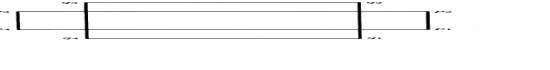
Figure 5: Conformally inequivalent rectangles; from [HS1].

2.4.2 The Incompatibility Theorem

Again consider the overlapping rectangles ${\Omega},{\Omega}^{\prime}$ of Fig. 5, and two combinatorially equivalent packings $P,P^{\prime}$ whose nerves triangulate the rectangles, as in Fig. 6. Assume for simplicity that the sets $D_{v}$ and $D^{\prime}_{v}$ of the packings are closed topological discs (except for the four sides $D_{1},...D_{4}$, $D_{1}^{\prime},...,D_{4}^{\prime}$ of the rectangles, which are considered to be sets of the packing). Intuitively, two topological discs $D$ and $D^{\prime}$ are called incompatible if they intersect as in Fig. 5. More formally, say that $D$ cuts $D^{\prime}$ if there are two points in $D^{\prime}\setminus{\rm interior}(D)$ that cannot be connected by a curve in ${\rm interior}(D^{\prime}\setminus D)$. Then Oded calls $D$ and $D^{\prime}$ incompatible if $D$ cuts $D^{\prime}$ or $D^{\prime}$ cuts $D.$ As he notes, the motivation for the definition comes from the simple but very important observation that the possible patterns of intersection of two circles are very special, topologically. Indeed, any two circles are compatible.

Theorem 2.10 ([S2], Theorem 3.1).

There is a vertex $v$ for which $D_{v}$ and $D^{\prime}_{v}$ are incompatible.

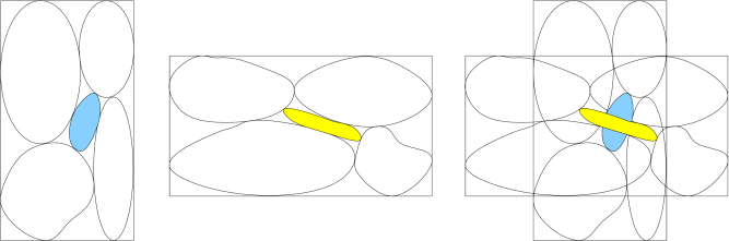
Figure 6: An incompatibility at the center.

Oded calls this result a combinatorial version of the modulus. However, it has rather little in common with the above notion of discrete modulus, except for the setup.

Oded’s clever proof by induction on the number of sets in the packing uses arguments from plane topology. An immediate consequence is that two rectangles cannot be packed by the same circle pattern, unless they have the same modulus $M$ and hence are similar: if they could, just place the two packings on top of each other as in Fig. 6 and obtain two incompatible circles, a contradiction. In the same vein, it is not difficult to reduce the proof of the rigidity Theorem 2.9 to an application of the incompatibility theorem.

2.4.3 A simple uniqueness proof

To end this section, here is a beautifully simple proof of the rigidity of finite circle packings whose nerve triangulates $S^{2}$. I copied it from the wikipedia (search for circle packing theorem), and believe it is due to Oded. As before, stereographically project the packing to obtain a packing of discs in the plane. This time, assume that the north pole belongs to the complement of the discs, so that the planar packing will consist of three “outer” circles and the remaining circles contained in the interstice between them.

“There is also a more elementary proof based on the maximum principle, which we now sketch. The key observation here is that if you look at the triangle formed by connecting the centers of three mutually tangent circles, then the angle formed at the center of one of the circles is monotone decreasing in its radius and monotone increasing in the two other radii. Consider two packings corresponding to G. First apply reflections and Möbius transformations to make the outer circles in these two packings correspond to each other and have the same radii. Next, consider a vertex v where the ratio between the corresponding radius in the one packing and the corresponding radius in the other packing is maximized. Since the angle sum formed at the center of the corresponding circles is the same (360 degrees) in both packings, it follows from the above observation that the radius ratio is the same at all the neighbors of v as well. Since G is connected, we conclude the radii in the two packings are the same, which proves uniqueness.”

2.5 Koebe’s Kreisnormierungsproblem

Koebe’s 1908 conjecture [Ko1] that every planar domain can be mapped conformally onto a circle domain is still open, despite considerable effort by Koebe and others. Important contributions were made by Grötzsch, Strebel, Sibner and others. One difficulty is the aforementioned lack of uniqueness. Another problem is that Theorem 2.5 is not true in the infinitely connected case, as the following example from [S6] illustrates: If $K=\{x+iy:x=0,\pm 1,\pm\frac{1}{2},\pm\frac{1}{3},...,y\in[-1,1]\}$, and if $D=\hat{\mathbb{C}}\setminus K$, then there is no conformal map $f$ of $D$, normalized by $f(z)-z\to 0$ as $z\to\infty,$ such that the component $\{iy:y\in[-1,1]\}$ of $\partial D$ corresponds to a horizontal line segment (or a point) while the other complementary components of $f(D)$ are vertical line segments. The same example also illustrates the fundamental continuity problem: There is a circle domain $D^{\prime}$ conformally equivalent to D, but the boundary component corresponding to $\{iy:y\in[-1,1]\}$ is just a point, so that the conformal map from $D^{\prime}$ to $D$ cannot be extended to the boundary.

The first joint paper of He and Schramm provided a breakthrough:

Theorem 2.11 ([HS1]).

If ${\Omega}$ has at most countably many boundary components, then ${\Omega}$ is conformally equivalent to a circle domain ${\Omega}^{\prime}$, and ${\Omega}^{\prime}$ is unique up to Möbius transformation.

Essentially, this result is still the strongest to date. Oded later [S6] gave a conceptually different and simpler proof based on his transboundary extremal length, which also applies to certain classes of domains with uncountably many boundary components.

The proof in [HS1] used transfinite induction and was based on the topological concept of the fixed-point index. I will illustrate the beautiful idea by sketching their proof of uniqueness. As it turned out, this argument for uniqueness had been given earlier by Strebel [Str]. The simple but crucial idea is to use the following (see [HS1], Lemma 2.2): If $f$ is a fixed-point free orientation preserving homeomorphism between two circles $C^{\prime}$ and $C^{\prime\prime}$, then the winding number of the curve $f(z)-z,z\in C^{\prime},$ around 0 is non-negative (recall Fig. 5 for a situation where the winding number is negative). Let $f:{\Omega}^{\prime}\to{\Omega}^{\prime\prime}$ be a conformal map and assume for simplicity that $f$ extends continuously to the boundary (in case of finitely many boundary components this is immediate from the reflection principle, but in the countable case this step is non-trivial), and that $f$ has no fixed points on the boundary. Composing with Möbius transformations, we may assume that $\infty\in{\Omega}^{\prime}$ and that $f(z)=z+a_{1}/z+a_{2}/z^{2}+\cdots.$ We want to show that $f$ is the identity. If not, denote $a_{j}$ the first non-zero Taylor coefficient, then $f(z)-z$ has winding number $-j$ as $z$ traverses a large circle $|z|=R,$ because $f(z)-z$ behaves like $a_{j}z^{-j}$. Moreover, each circular boundary component maps to a circular component. These boundary components are oriented negatively (to keep the domain to the left) and thus, by the above crucial idea, contribute a non-positive number to the winding of $f(z)-z,z\in\partial({\Omega}\cap\{|z|\leq R\}$ around 0. Hence the total winding number is negative, contradicting their generalization of the argument principle (the winding number counts the number of zeroes of $f(z)-z.$) Of course, I have swept most details under the rug, most notably the proof of continuity based on a powerful generalization of Schwarz’ Lemma to circle domains (Theorem 0.6 in [HS1]).

Combining the fixed-point index method of [HS1] with an analysis of quasiconformal deformations using the reflection group approach and Sullivan’s rigidity theorems, He and Schramm [HS4] improve Theorem 2.11 to domains ${\Omega}$ for which all boundary components are circles or points except those in a countable and closed family. They also obtain the following generalization of the Riemann mapping theorem. Let $A\subseteq{\mathbb{C}}$ be simply connected.

Theorem 2.12 ([HS4],[HS5]).

If ${\Omega}\subset A$ is a relative circle domain (each connected component of $A\setminus{\Omega}$ is a point or a closed disc), then there is a relative circle domain ${\Omega}^{*}$ in ${\mathbb{D}}$ conformally equivalent to ${\Omega}$, and so that $\partial A$ corresponds to $\partial{\mathbb{D}}.$ Conversely, if ${\Omega}^{*}$ is a relative circle domain in ${\mathbb{D}}$, there is such ${\Omega}\subset A.$

The converse direction is the main result of [HS5].

2.6 Convergence to conformal maps

Let us return to the setting of the Rodin-Sullivan Theorem 2.3 about convergence of the discrete map $f_{\varepsilon}$ to the conformal map $f.$ Consider the piecewiese linear extension of $f_{\varepsilon}$ from the carrier of $P$ to the carrier of $P^{\prime}$ that maps equilateral triangles to the corresponding triangles (formed by the centers of $P^{\prime}$). By the elementary “Ring Lemma” of [RSu], the angles of these triangles are bounded away from $0$ and $\pi$ (so that $f_{\varepsilon}$ is quasiconformal with dilation uniformly bounded above). At the heart of the Rodin-Sullivan proof is the uniqueness of the hexagonal packing as the only packing in the plane with nerve the triangular lattice (see the discussion in Section 2.4). It rather easily implies that tangent circles centered in a compact set of ${\Omega}$ correspond to tangent circles in ${\mathbb{D}}$ whose radii are asymptotically equal as $\varepsilon\to 0.$ Hence the triangles in $P^{\prime}$ are nearly equilaterals when $\varepsilon$ is small (the angles tend to $\pi/3$), so that $f_{\varepsilon}$ is nearly angle preserving in each triangle. Now the theory of quasiconformal maps readily yields equicontinuity of the family of maps $f_{\varepsilon}$, and shows that every subsequential limit $\lim f_{\varepsilon_{j}}$ is a conformal map. The theorem follows from uniqueness of normalized conformal maps.

He’s thesis [He] provided a quantitative estimate for the rate of convergence of the angles (the difference to $\pi/3$ is $O({\varepsilon}$)). This estimate was known to imply convergence of the ratio of corresponding radii $\rm{rad}(D^{\prime})/\rm{rad}(D)$ to the absolute value $|f^{\prime}|$ of the derivative. A probabilistic proof of $C^{0}$ (locally uniform) convergence of circle packings was given by Stephenson [Ste1]. Convergence of $f_{\varepsilon}$ to $f$ for packings other than the hexagonal was proved in [HR], under the assumption of bounded valency of the graph. In [DHR], the quality of convergence was improved to convergence in $C^{2}$ (that is, convergence of first and second derivatives; strictly speaking, instead of $f_{\varepsilon}$ they considered the “piecewise Möbius” map that sends interstices between triples of mutually tangent circles to the corresponding interstices). He and Schramm [HS6] found an elementary new convergence proof, based on the topological ideas discussed above and thus avoiding quasiconformal maps. Their proof also gave convergence up to $C^{2}$, and worked in a more general setting. In particular, it does not need the assumption of uniformly bounded degree of [HR].

In the remarkable paper [HS8], He and Schramm proved $C^{\infty}$-convergence of hexagonal disk packings to the Riemann map:

Theorem 2.13 ([HS8], Theorem 1.1).

The discrete functions $f_{\varepsilon}:V_{\varepsilon}\to{\mathbb{D}}$ converge in $C^{\infty}$ to the Riemann mapping $f:{\Omega}\to{\mathbb{D}}$, in the sense that the discrete partial derivatives of $f_{\varepsilon}$ of any order converge locally uniformly to the corresponding partial derivatives of $f$.

The discrete first-order derivatives for $v\in V_{\varepsilon}$ are

$$\partial_{\varepsilon,k}f_{\varepsilon}(v)=\varepsilon^{-1}(f_{\varepsilon}(v+\varepsilon\ \omega^{k})-f_{\varepsilon}(v)),$$

where $k\in{0,1,...,5}$ and $\omega=(1+i\sqrt{3})/2$ is a $6-$th root of unity. In particular, it follows that $(\partial_{\varepsilon,0})^{k}f_{\varepsilon}$ converges to the $k-$th derivative $f^{(k)}$ locally uniformly on $G$.

The Schwarzian derivative

$$S(f)(z)=\frac{f^{\prime\prime\prime}(z)}{f^{\prime}(z)}-\frac{3}{2}\frac{f^{\prime\prime}(z)^{2}}{f^{\prime}(z)^{2}}$$ (2)

of a locally univalent analytic function measures the deviation of $f$ from a Möbius transformation, in particular $S(f)\equiv 0$ if $f$ is Möbius. A key idea in the proof is to define a discrete analog of the Schwarzian derivative, to compute the (discrete) Laplacian of this Schwarzian, and to employ a regularity theorem for discrete elliptic equations to obtain boundedness of all partials of the Schwarzian. The definition of the discrete Schwarzian is the circle packing analog of an invariant that Oded so masterfully employed in his earlier work [S8] on circle patterns with the combinatorics of the square grid.

2.7 Other topics

Oded’s approach to both mathematics and to life was extraordinarily innovative and unaccepting of conventions. Notions that most people take for granted without even thinking about, he would open-mindedly question, often coming up with amazing alternative solutions. For example, I would not even think about camping on the foot of a glacier without a sleeping bag. Climbing little Tahoma peak with Oded, he proved to me that even this idea can be pursued. It was perhaps one of his less successful innovations, though.

In the lovely paper [S5], Oded shows that for each triangulation $G$ of a quadrilateral, there is a packing of a rectangle $R$ by (horizontal) squares with the combinatorics of $G$ (a square might degenerate to a point, as in Figure 7).

Figure 7: A triangulation and the associated square packing. Thanks to David Wilson for providing this figure from [S5]

The packing is actually a tiling: Indeed, Oded points out the following simple observation.

Let $P_{a}$, $P_{b},$ $P_{c}$ be three rectangles whose edges are parallel to the coordinate axis. Suppose that the intersection of every two of these rectangles is nonempty. Then $P_{a}\cap P_{b}\cap P_{c}\neq\emptyset.$

The same tiling theorem was obtained independently by Cannon, Floyd and Parry in [CFP1]. Both employ Cannon’s discrete extremal length (see Section 2.4.1) and obtain the side lengths $s(v)$ of the squares as the weights $\rho(v)$ of the extremal metric (corresponding to the family of “combinatorial curves” joining two opposite sides of the quadrilateral). It is quite different from the classical square packings of Brooks, Smith, Stone and Tutte [BSST], in particular, since the metrics considered here live on the vertices rather than the edges of the graph.

A very similar idea is exploited in the important paper [S6]. The classical setting of extremal length (recall (1)) is a family $\Gamma$ of curves contained in a domain ${\Omega}.$ Invariance

$$\lambda(f(\Gamma))=\lambda(\Gamma)$$

under conformal maps of ${\Omega}$ is almost trivial (just pull back metrics from $f({\Omega})$). Oded’s notion of transboundary extremal length $\lambda_{\Omega}(\Gamma)$ applies to curve families $\Gamma$ that are not necessarily contained in ${\Omega}.$ The metrics are now replaced by generalized metrics $\rho$ that, roughly speaking, also assign length to complementary components. The length $\int_{\gamma}\rho|dz|$ is replaced by $\int_{\gamma\cap{\Omega}}\rho|dz|+\sum_{p}\rho(p)$ if $\gamma$ is not contained in ${\Omega},$ where the sum is over all boundary components of ${\Omega}$ that $\gamma$ meets. Then the definition is $\lambda_{\Omega}(\Gamma)=\sup_{\rho}(\inf_{\gamma}\int_{\gamma\cap{\Omega}}\rho|dz|+\sum_{p}\rho(p))/\int_{{\mathbb{C}}}\rho^{2}dxdy$, and conformal invariance is again immediate. Using this innocent looking extension, Oded provides an elegant self-contained proof of the countable Koebe conjecture, and moreover is able to deal with the case of domains for which the complementary component satisfy a certain fatness condition (${\rm area}(A\cap B(x,r))\geq cr^{2}$ for each component $A$, each $x\in A$ and each disc $B(x,r)$ that does not contain $A$).

Circle packings corresponding to infinite graphs $G$ can be obtained by taking Hausdorff limits of packings corresponding to finite subgraphs, but where do they “live”? Beardon and Stephenson [BSt1],[BSt2] have shown, under the assumption that the degrees of the vertices are uniformly bounded, that the carrier of such a packing is either the plane (call this case parabolic), or that it can be chosen to be the disc (hyperbolic). They also showed that both cases are mutually exclusive, and that the packing is hyperbolic if each degree is at least seven. The uniform boundedness assumption was later removed by He and Schramm [HS1], and they proved in general that the type of a packing is unique (that is, there is no infinite graph that packs both the disc and the plane). In the impressive paper [HS3], they characterize the type in terms of the discrete extremal length, and use it to show that the packing is parabolic if simple random walk on $G$ is recurrent. They conclude (Theorem 10.1) that a packing is parabolic if at most finitely many vertices have degree greater than 6 (notice that every vertex of the hexagonal packing has degree 6). This paper contains their earlier result [HS3b] that a packing is hyperbolic if the lower average degree is greater than 6. By definition, the lower average degree is

$${\rm lav}(G)=\sup_{W_{0}}\inf_{W\supset W_{0}}\frac{1}{|W|}\sum_{v\in W}{\rm deg}(v).$$

In the case that the degrees of the vertices are uniformly bounded, they also show that transience implies hyperbolicity. Jointly with Itai Benjamini, this line of investigation was carried further in [BS1] and [BS2], by applying circle- and square packings to constructions of harmonic functions on graphs. Another nice application of circle packings is the recurrence of (weak) limits of random planar graphs with bounded degree, [BS2].

I have always admired Oded’s ability to find a good modification of a difficult problem that turns it into a tractable problem while keeping its essential features. One of the many examples is his work on discrete analytic function [S8]. Since circle packings can be viewed as discrete analogs of conformal maps, it is natural to ask for the analogs of analytic functions, thus giving up injectivity (disjointness of the discs). See [Ste2] for the state of the art and beautiful illustrations. Peter Doyle described collections of discs that are tangent according to the hexagonal pattern that are analogs of the exponential function. He conjectured that these would be the only “entire” circle packing immersions. While Oded was not able to resolve this conjecture, he did find that collections of overlapping discs based on the square grid seem better suited for the problem, and constructed the analog of the error function $\int e^{-z^{2}}dz$ in this setting. Along the way, he introduced Möbius invariants that are discrete analogs of the Schwarzian derivative and became instrumental in his later work [HS8].

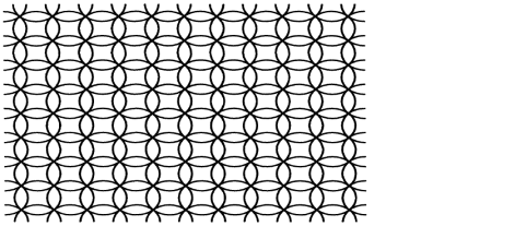
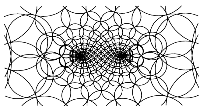
Figure 8: The square grid and the $\sqrt{i}$SG erf pattern, from [S8]

3 The Schramm-Loewner Evolution

There are several excellent lecture notes, overview articles, and a textbook on SLE [La3], mostly by and for probabilists or theoretical physicists, see [BB3], [Car2], [Dup], [GK], [KN], [S11], [W1], [W2] and the references therein. It is not my intention to provide another streamlined introduction to the area. Instead, I would like to give a somewhat historic account with an emphasis on Oded’s contributions, highlighting some of the mathematical challenges he faced.

3.1 Pre-history

It is perhaps appropriate to very briefly describe the state of knowledge related to conformally invariant scaling limits prior to Oded’s discovery of SLE, and to describe some of the results that were instrumental in his work. Oded’s own historical narrative is Section 1.2 in [S11].

Two-dimensional lattice processes such as the Self-Avoiding Walk (SAW), the Ising model, percolation, and diffusion limited aggregation (DLA), to name just a few, have been intensively studied by physicists and by probabilists for a long time. See Figure 21 for some pictures, and the aforementioned articles for descriptions of the models. In the physics community, many problems such as finding the Hausdorff dimension of scaling limits of these sets were considered well-understood. The implicit assumption of conformal invariance of the scaling limit allowed the use of the powerful machinery of conformal field theory and led to results such as Cardy’s formula for the crossing probability of critical percolation [Car1]. On the mathematical side, progress was much slower, one of the hurdles being that in most cases the existence of a scaling limit was unknown. Even finding suitable definitions of the concept of scaling limit was a nontrivial task.

In the late 1980’s, Christian Pommerenke told me how compositions of (random) conformal maps onto slitted discs could be viewed as a variant of the Witten-Sander model for DLA [WS]. At the same time, Richard Rochberg and his son David were working on this setup. It seems that the only trace of this is a talk given by Rochberg at the March 1990 AMS Regional meeting in Manhattan, Kansas, titled “Stochastic Loewner Equation”. Their model is similar to an approach to Laplacian growth proposed by Hastings and Levitov [HL], and is quite different from what is now called Stochastic Loewner Evolution or Schramm-Loewner Evolution SLE. At that time, other analysts such as Lennart Carleson, Peter Jones and Nick Makarov worked with similar ideas, see e.g. [CM]. Oded was at best dimly aware of these activities, and was not really interested in stochastic processes such as DLA until much later.

Greg Lawler’s invention [La] of the Loop Erased Random Walk (LERW) provided the mathematics community with a process that shared some features with the Self-Avoiding Walk, but at the same time was more tractable, partly due to its Markovian property. Pemantle’s work [Pe] and Wilson’s algorithm provided a link between Uniform Spanning Trees (UST) and LERW’s. Intensive research on the UST [Ly] culminated in the paper [BLPS] by Benjamini, Lyons, Peres and Schramm. The deep work of Rick Kenyon [Ke1] combined powerful combinatorics and discrete complex analysis and exhibited conformal invariance properties of the LERW. He was also able to determine its expected length.

3.2 Definition of SLE

Oded told me in 1997 about his idea to exploit conformal invariance in order to study the LERW. The streamlined way to present SLE in courses or texts, beginning with a crashcourse on the Loewner equation followed by a crash course on stochastic calculus (or the other way round) is, of course, not quite representative of its emergence. In a 2006 email exchange with Yuval Peres and myself about the history of SLE, Oded wrote:

Up to the time when I started thinking about SLE, I did not really know what Loewner’s equation was, or what was the idea behind it, though I did know that it was a tool which was important for the coefficients problem and that it involved slit mappings and a differentiation in the space of conformal maps. I kind of rediscovered it in the context of SLE and then made the connection.

3.2.1 The (radial) Loewner equation

Loewner ([Lo]; see also [Dur],[Po2] or [La3]) introduced his differential equation as a tool in his attempt to prove the Bieberbach conjecture $|a_{n}|\leq n$ concerning the Taylor coefficients of normalized conformal maps $f(z)=z+\sum_{n=2}^{\infty}a_{n}z^{n}$ of the unit disc. It was also instrumental in the final solution by de Branges in 1984.

Let ${\gamma}$ be a simple path that is contained in ${\mathbb{D}}$ except for one endpoint on $\partial{\mathbb{D}}.$ More precisely, let ${\gamma}:[0,\tau]\to\overline{\mathbb{D}}$ be continuous and injective with ${\gamma}(0)\in\partial{\mathbb{D}}$ and ${\gamma}(\tau)=0$, such that ${\gamma}(0,\tau]\subset{\mathbb{D}}.$ Denote $G_{t}={\mathbb{D}}\setminus{\gamma}[0,t]$ so that $G_{0}={\mathbb{D}}.$ Then, for each $0\leq t<\tau$, there is a unique conformal map $g_{t}:G_{t}\to{\mathbb{D}}$ that is normalized by $g_{t}(0)=0$ and $g_{t}^{\prime}(0)>0.$ By Schwarz’ Lemma, $g_{t}^{\prime}(0)$ strictly increases, $g_{0}^{\prime}(0)=1,$ and it is not hard to see that $g_{t}^{\prime}(0)\to\infty$ as $t\to\tau.$ Hence we can reparametrize $\gamma$ so that $\tau=\infty$ and $g_{t}^{\prime}(0)=e^{t}$. Loewner’s theorem says that

$$\frac{\partial}{\partial t}g_{t}(z)=g_{t}(z)\frac{{\zeta}_{t}+g_{t}(z)}{{\zeta}_{t}-g_{t}(z)}$$ (3)

for all $t\geq 0$ and all $z\in G_{t}$, where the “driving term”

$${\zeta}_{t}=g_{t}({\gamma}(t))\in\partial{\mathbb{D}}$$

is continuous (a priori, $g_{t}$ is only defined in $G_{t}$, but it can be shown that $g_{t}$ extends to ${\gamma}(t)$).

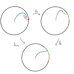
Figure 9: Conformal maps from slit discs onto discs.

A simple but crucial observation is that the driving term ${\zeta}^{T}$ of the curve ${\gamma}^{T}=g_{T}(\gamma)$ (more precisely, the parametrized curve $\gamma^{T}(s):=g_{T}(\gamma(T+s))$) is given by ${\zeta}^{T}_{s}={\zeta}_{T+s}.$ Thus “conformally pulling down” a portion of ${\gamma}$ corresponds to shifting the driving term. Intuitively, one can think of the Loewner equation as describing a conformal map to a slitted disc as a composition of conformal maps onto infinitesimally slitted discs with slit at $\zeta_{t},$ plus the statement that the conformal map onto such a disc is $z\mapsto z+z\frac{{\zeta}_{t}+z}{{\zeta}_{t}-z}\Delta t$ up to first order in $\Delta t$.

Thus the Loewner equation associates with each simple curve ${\gamma}\subset{\mathbb{D}}$ a continuous function ${\zeta}_{t}$ with values in $\partial{\mathbb{D}}.$ Conversely, it is not hard to show that the solution $g_{t}(z)$ to the initial value problem (3), $g_{0}(z)=z,$ forms a family of conformal maps of simply connected domains $G_{t}$ onto ${\mathbb{D}}.$ In fact, $G_{t}$ is the set of those points ${\zeta}\in{\mathbb{D}}$ for which the solution is well-defined on the interval $[0,t]$. It easily follows that $G_{t}$ increases in $t,$ and that $z\in G_{t}$ unless $g_{s}(z)=\zeta_{s}$ for some $s\leq t.$ The complement

$$K_{t}={\mathbb{D}}\setminus G_{t}$$

is called the hull of ${\zeta}.$ In our original setup of a slit disc, we simply recover the curve, $K_{t}={\gamma}[0,t].$ It has been known since Kufarev [Ku] that smooth functions ${\zeta}$ generate smooth curves ${\gamma},$ but that there also exist continuous functions ${\zeta}$ for which the associated hull is not a simple arc in ${\mathbb{D}}$. Kufarev’s example simply is the computation that a circular chord ${\gamma}$ of the unit circle has continuous driving term. In fact, it can be topologically wild (not locally connected), see [MR]. My own interest in the Loewner equation originated when Oded asked me which driving terms generate curves.

3.2.2 The scaling limit of LERW

The LERW is obtained from simple random walk by erasing loops chronologically.

Figure 10: A loop erased random walk in the disc, from [S9].

The main result of Oded’s celebrated paper [S9] was a conditional theorem: Assuming the existence and conformal invariance of the scaling limit of LERW, he showed that the Loewner driving term of the resulting (random) limiting curve is a Brownian motion on the unit circle, ${\zeta}_{t}=e^{iB_{2t}}.$ To make this rigorous, he first gave the following definition of the notion of scaling limit: Let $D\subsetneq{\mathbb{C}}$ be a domain, fix $a\in D$, and for $\delta>0$, consider the LERW on the graph $\delta{\mathbb{Z}}^{2}\cap D$, started at a point closest to $a$ and stopped when reaching $\partial D.$ Viewing the path of the LERW as a random subset of the sphere $S^{2}={\mathbb{C}}\cup\{\infty\}$, its distribution is a discrete measure $\mu_{\delta}$ on the space of compact subsets of $S^{2}$. Equipped with the Hausdorff distance, the space of compact subsets of $S^{2}$ is a compact metric space, and so is the space of its Borel measures. The existence of subsequential weak limits $\mu=\lim_{j}\mu_{\delta_{j}}$ follows at once. If the limit measure $\mu=\lim_{\delta\to 0}\mu_{\delta}$ exists, it is called the scaling limit of LERW from $a$ to $\partial D$.

Theorem 3.1 ([S9], Theorem 1.1).

If each connected component of $\partial D$ has positive diameter, then every subsequential scaling limit measure $\mu$ of the LERW from $a$ to $\partial D$ is supported on simple paths.

In other words, the measure of the set of non-simple curves is zero. This theorem is interesting in its own right. It has been known previously that, loosely speaking and under mild assumptions, random curves have uniform continuity properties that imply their (subsequential) scaling limits to be supported on continuous curves [AB]. However, the fact that the loop erased paths are simple curves does not directly imply that the limiting objects have no loops. Indeed, the limits of other discrete random simple curves such as the critical percolation interface or the uniform spanning tree Peano path are not simple. The proof uses estimates for the probability distribution of “bottlenecks”, based on harmonic measure estimates and Wilson’s algorithm, and a topological characterization of simple curves.

Next, Oded formulated the conjecture of existence and conformal invariance of the scaling limit as follows.

Conjecture ([S9],1.2) Let $D\subsetneqq{\mathbb{C}}$ be a simply connected domain in ${\mathbb{C}}$, and let $a\in D$. Then the scaling limit of LERW from $a$ to $\partial D$ exists. Moreover, suppose that $f:D\to D^{\prime}$ is a conformal homeomorphism onto a domain $D^{\prime}\subset{\mathbb{C}}$. Then $f_{*}\mu_{a,D}=\mu_{f(a),D^{\prime}}$, where $\mu_{a,D}$ is the scaling limit measure of LERW from $a$ to $\partial D$, and $\mu_{f(a),D^{\prime}}$ is the scaling limit measure of LERW from $f(a)$ to $\partial D^{\prime}$.

The most important and exciting result of [S9] was the insight that this conjecture implied an explicit construction of the limit in terms of the Loewner equation. By Theorem 3.1, the conjectural scaling limit $\mu$ induces a measure on the space of continuous real-valued functions ${\hat{\zeta}}_{t}$ via the correspondence ${\gamma}\mapsto{\zeta}=e^{i{\hat{\zeta}}}$ of the Loewner equation. Oded showed that the law of ${\hat{\zeta}}$ is that of a time-changed Brownian motion, $B_{2t}$:

Theorem 3.2 ([S9], Theorem 1.3).

Assuming the above conjecture, the scaling limit $\mu$ is equal to the law of the hulls $K$ associated with the driving term ${\zeta}=e^{iB_{2t}}$, where $B_{t},t\geq 0$ is a Brownian motion started at a uniform random point in $[0,2\pi)$.

In his characteristic way, Oded pointed out the simple idea behind the theorem. From his paper:

At the heart of the proof of Theorem 3.2 lies the following simple combinatorial fact about LERW. Conditioned on a subarc ${\beta}^{\prime}$ of the LERW ${\beta}$ from 0 to $\partial D$, which extends from some point $q\in{\beta}$ to $\partial D$, the distribution of ${\beta}\setminus{\beta}^{\prime}$ is the same as that of LERW from 0 to $\partial(D-{\beta}^{\prime})$, conditioned to hit $q$. When we take the scaling limit of this property, and apply the conformal map from $D-{\beta}^{\prime}$ to ${\mathbb{D}}$, this translates into the Markov property and stationarity of the associated Löwner parameter ${\zeta}$.

He also notes that “the passage to the scaling limit is quite delicate”. The translation into the Markov property and stationarity is by means of the aforementioned principle that “conformally pulling down” a portion ${\gamma}^{\prime}$ of ${\gamma}$ corresponds to shifting the driving term. Thus ${\hat{\zeta}}$ is a continuous process with stationary and independent increments. Now the theory of Levy processes (and the symmetry of LERW under reflection) implies that ${\hat{\zeta}}_{t}$ has the law of $\sqrt{\kappa}B_{t}$ for some $\kappa>0$ and a standard Brownian motion $B$. It remained to determine the constant $\kappa.$ To this end, Oded gives the following

Definition. The (radial) stochastic Loewner evolution $SLE_{\kappa}$ with parameter $\kappa>0$ is the random process of conformal maps $g_{t}$ generated by the Loewner equation driven by ${\zeta}_{t}=e^{i\sqrt{\kappa}B_{t}}.$

In Section 7 of [S9] he actually defined SLE as a process of random paths generated by the Loewner equation, and therefore had to restrict to those values of $\kappa$ for which the resulting hulls are simple curves; he conjectured that this is the interval $[0,4]$.

Next, he analyzed the winding number of the SLE-path around 0, and of the LERW: If $\theta_{\kappa}(t)=\arg{\gamma}(t)$, $t\geq 0$, denotes the continuously defined argument along the curve, then he computed the variance

$$E[\theta_{\kappa}(t)^{2}]=(\kappa+o(1))\log t.$$

It follows that the winding number of the portion of the SLE path until its first hitting of the circle of radius $\varepsilon$ centered at $0$ has variance $(\kappa+o(1))\log(1/\varepsilon).$ On the other hand, Kenyon’s work [Ke2] implies that the variance of the winding number of LERW in ${\mathbb{D}}\cap\varepsilon{\mathbb{Z}}^{2}$ is $(2+o(1))\log(1/\varepsilon),$ and after some work the conclusion $\kappa=2$ follows.

Oded went on to compute what he called the critical value for SLE: He proved that for $\kappa>4,$ almost surely SLE will not generate simple paths, and conjectured that it will for $\kappa\in[0,4]$. See the discussion in Section 3.3.3 for the simple proof using Ito’s formula (in the chordal case). However, Oded was a self-taught newcomer to stochastic calculus, discovered some of the basics himself, and commented on his proof in an email in January 1999:

This must all be quite standard, to people with the right background. But not for me.

3.2.3 The chordal Loewner equation, percolation, and the UST

The classical (radial) Loewner equation is well-suited for curves that join an interior point to a boundary point, such as curves generated by the LERW. Other processes generate curves joining two boundary points. Oded realized how important the “correct” normalizations are in dealing with conformal maps and in particular the Loewner equation, and found the appropriate variant of the Loewner equation (it turned out later that this version has been described earlier, beginning with N.V. Popova [Pop1],[Pop2]; I would like to thank Alexander Vasiliev for this reference). He describes this in another email in January 1999:

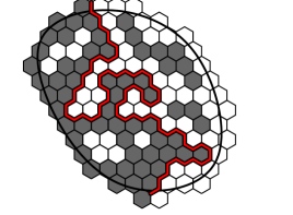
Figure 11: Percolation in a domain, from [S11].

I have a mathematical querry. Before the question itself, here’s the motivation. For the LERW scaling limit, the natural object is a probability measure on the set of paths from a point in the domain to the boundary. In other settings, the natural object is a probability measure joining two points on the boundary of a domain. Consider, for example, percolation in the unit disk. Let $(\gamma,\beta)$ be a partition of the boundary of the disk to two arcs, disjoint except for the endpoints. Let $K$ be the union of all percolation clusters inside the disk that are connected to $\gamma$. Then the outer boundary of $K$ is a path, $\alpha$, joining the two endpoints of $\gamma$. The scaling limit of $\alpha$ is conjecturally conformally invariant (but not a simple path). Assuming conformal invariance, I’m optimistic that the scaling limit can be represented by a Loewner-like Brownian evolution. The first step for this seems to be the following variation on Loewner’s theorem:

Thm: Let $\alpha:[0,\infty)\to{\mathbb{C}}$ be a continuous simple path such that $\alpha(0)=0,\lim_{t\to\infty}\alpha(t)=\infty$ and $\operatorname{Im}(\alpha(t))>0$ when $t>0.$ Let $f_{t}$ be the conformal map from the upper half plane to the upper half plane minus $\{\alpha(s):0\leq s\leq t\}$, which is normalized by $f_{t}(z)=z+O(1/z)$ near infinity. By change of parameterization of $\alpha$ (and perhaps changing its interval of definition), we may assume that $f_{t}(z)=z+t/z+O(1)/z^{2}$ near infinity. Set $g(w,t)=f_{t}^{-1}(w)$. Then $\{\partial g/\partial t\}=1/(g-k(t))$, where $k(t)=g(\alpha(t),t).$

In the situation of percolation and related conformal invariance models, one should expect $k(t)=cBM(t)$, where BM is on the real line. Have you seen this theorem? The proof should not be difficult. It can either be derived from Loewner’s theorem, or by adapting the proof.

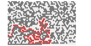
Figure 12: The percolation exploration path

In order to coincide with the normalization of the radial Loewner equation, he later slightly adjusted the parametrization of the path $\alpha$ so that

$$f_{t}(z)=z+2t/z+O(1)/z^{2}$$

and

$$\frac{\partial}{\partial t}g_{t}(z)=\frac{2}{g_{t}(z)-W_{t}}.$$ (4)

With this normalization and assuming conformal invariance of the percolation scaling limit, he showed that the (non-simple) limit curves would satisfy the chordal Loewner equation (4) with $W_{t}=\sqrt{6}B_{t}$. The value 6 can be found as the only $\kappa$ such that the random sets generated by $\sqrt{\kappa}B_{t}$ satisfy Cardy’s formula, or the locality property discussed below. This led to the definition of chordal $SLE_{\kappa}$ as the random process of conformal maps

$$g_{t}:{\mathbb{H}}\setminus K_{t}\to{\mathbb{H}}$$

generated by the Loewner equation (4) with driving function $W(t)=\sqrt{\kappa}B_{t}$, where $B$ is a standard Brownian motion.

The hull $K_{t}$ is the set of those points $z$ for which $g_{s}(z)=W_{s}$ for some $s\leq t$ so that (4) becomes undefined. Since $g_{t}$ is determined by $K_{t},$ one has the equivalent

Definition: Chordal $SLE_{\kappa}$ is the process of random hulls $(K_{t},t\geq 0)$ generated by the Loewner equation (4) with $W_{t}=\sqrt{\kappa}B_{t}$.

In the same paper, Oded also defines and analyzes subsequential scaling limits of the uniform spanning tree. He ends the paper by speculating (that is, stating without giving detailed proofs) about the Loewner driving term of the UST Peano curve in the upper half plane ${\mathbb{H}}$. He finds that, again assuming existence and conformal invariance of the limit, this random space filling curve is $SLE_{8}$. At the end of the introduction, he summarizes the findings of the paper as follows:

The emerging picture is that different values of $\kappa$ in the differential equation (3) or (4) produce paths which are scaling limits of naturally defined processes, and that these paths can be space-filling, or simple paths, or neither, depending on the parameter $\kappa$.

Figure 13: The UST Peano curve, from [RoS].

3.3 Properties and applications of SLE

Two exciting developments took place shortly after the introduction of SLE, namely the very productive collaboration of Greg Lawler, Oded Schramm and Wendelin Werner, and the surprising proof of existence and conformal invariance of the percolation scaling limit by Stas Smirnov. I will begin describing the former, and defer the latter to Section 3.3.4.

3.3.1 Locality

In the important papers [LW1] and [LW2], Lawler and Werner discovered that Brownian excursions have a certain restriction property (explained below), and that intersection exponents of conformally invariant processes with this property are closely related to those of Brownian motion. What was missing was a way to compute exponents of some conformally invariant process. Lawler, Schramm and Werner discovered that SLE provided such a process to which the universality arguments of Lawler and Werner [LW2] applied. The following email from Oded describes the crucial property:

I don’t remember if I’ve mentioned to you the restriction property for SLE(6) that Greg, Wendelin and I have proved. It says that (up to time parameterization) the law of SLE(6) in an arbitrary domain D starting from a point p on the boundary and stopped when it exits a small ball B around p, does not depend on the shape of the domain outside B (provided that D-B is connected, say). Thus, SLE(6) is purely a local process, like BM. This is not true for $\kappa\neq 6$. For example, SLE(6) in the disk (with Loewner’s original equation) is the same as SLE(6) in the half plane, with my variation on Loewner’s equation. This seems to say that SLE(6) is a very special process.

The above property is trivial for the discrete critical percolation exploration path, since the path can be grown “dynamically” by deciding the color of a hexagon only when the path meets it and needs to decide whether to turn “right” or “left”. Hence, in light of the conjectured scaling limit, locality for chordal $SLE_{6}$ was not unexpected. The coincidence of chordal and radial $SLE_{6}$, discussed below, was more surprising.

Here is a precise statement of the locality property. Let $D={\mathbb{H}}\setminus A$ be a simply connected subdomain of ${\mathbb{H}}$ such that $A$ is bounded and also bounded away from $0.$ Denote $g_{A}$ the conformal map from $D$ onto ${\mathbb{H}}$ with the hydrodynamic normalization ($g_{A}(z)-z\to 0$ as $z\to\infty$), and set $\Phi_{A}=g_{A}-g_{A}(0).$ Then SLE in $D$ from $0$ to $\infty$ is defined as the preimage of SLE in ${\mathbb{H}}$ from $0$ to $\infty$ under $\Phi_{A}$. The following expresses the fact that SLE in $D$ is a time-change of SLE in ${\mathbb{H}}$, up to the time that the process hits $A$. Let $T=\inf\{t:K_{t}\cap A\neq\emptyset\}$ and $\tilde{T}=\inf\{t:K_{t}\cap\Phi_{A}(\partial A)\neq\emptyset\}$.

Theorem 3.3 ([LSW2], Theorem 2.2).

For $\kappa=6,$ the processes $(\Phi_{A}(K_{t}),t<T)$ and $(K_{t},t<\tilde{T})$ have the same law, up to re-parametrization of time.

The equivalence of chordal and radial $SLE_{6}$ was established in [LSW3], Theorem 4.1: Define the hulls $K_{t}$ of chordal $SLE_{\kappa}$ in ${\mathbb{D}}$ from $1$ to $-1$ as the image of chordal $SLE_{\kappa}$ in ${\mathbb{H}}$, under the conformal map $f(z)=(i-z)/(i+z)$. Thus $K_{t}$ are hulls growing from 1 towards -1 in $\overline{\mathbb{D}}.$ Denote $T\leq\infty$ the first time when $K_{t}$ contains $0.$ Similarly, denote $\widetilde{K}_{t}$ the chordal $SLE_{\kappa}$ hulls in ${\mathbb{D}}$, started at $1,$ and denote $\widetilde{T}$ the first time when $\widetilde{K}_{t}$ contains $-1.$ Then, for $\kappa=6,$ the laws of $(K_{t},t<T)$ and $(\widetilde{K}_{t},t<\widetilde{T})$ are the same, up to a random time change $s=s(t)$. The proof and Girsanov’s theorem also show that for all values of $\kappa,$ the laws of $K_{t}$ and $\widetilde{K}_{s(t)}$ are equivalent (in the sense of absolute continuity of measures), if $t$ and $\widetilde{t}$ are bounded away from $T$ and $\widetilde{T}.$ See Proposition 4.2 in [LSW3].

The first proof of the locality Theorem 3.3 was rather long and technical, based on an analysis of the Loewner driving function of a curve under continuous deformation of the surrounding domain. A different and simpler proof was found later (see Proposition 5.1 in [LSW8]), by analyzing $\tilde{W}_{t}:=h_{t}(W_{t}),$ where $h_{t}:=\tilde{g}_{t}\circ g_{A}\circ g_{t}^{-1}$ and $\tilde{g}_{t}=g_{g_{t}(D\setminus K_{t})}$ is the normalized conformal map of $g_{t}(D\setminus K_{t})$ to ${\mathbb{H}}$. Writing

$$\tilde{g}_{t}(z)=z+\frac{a_{t}}{z}+O(\frac{1}{z^{2}}),$$

computation shows that

$$\partial_{t}\tilde{g}_{t}(z)=\frac{\partial_{t}a_{t}}{\tilde{g}_{t}(z)-\tilde{W}_{t}}=\frac{2h_{t}^{\prime}(W_{t})^{2}}{\tilde{g}_{t}(z)-\tilde{W}_{t}}.$$

With $W_{t}=\sqrt{\kappa}B_{t}$, computation using Ito’s formula shows

$$d\tilde{W}_{t}=h_{t}^{\prime}(W_{t})dW_{t}+\bigl{(}(\kappa/2)-3\bigr{)}h_{t}^{\prime\prime}(W_{t})dt.$$ (5)

Thus $\tilde{W}_{t}$ is a local martingale if (and only if) $\kappa=6,$ and a time change shows that $(\tilde{g}_{t},t\geq 0)$ is $SLE_{6}$.

3.3.2 Intersection exponents and dimensions

The locality of $SLE_{6}$ has been used to determine the so-called intersection exponents of 2-dimensional Brownian motion, and to compute the Hausdorff dimensions of various sets associated with its trace. These results established Schramm’s SLE and the Lawler-Werner universality arguments as a fundamental and powerful new tool.

If $B^{1}_{t}$ and $B^{2}_{t}$ are two independent planar Brownian motions started at two different points $B^{1}_{0}\neq B^{2}_{0},$ it easily follows from the subadditivity of $t\mapsto\log{\mathbb{P}}[B^{1}[0,t]\cap B^{2}[0,t]=\emptyset]$ that there is a number ${\zeta}>0$ such that

$${\mathbb{P}}[B^{1}[0,t]\cap B^{2}[0,t]=\emptyset]=\left(\frac{1}{t}\right)^{{\zeta}+o(1)}.$$

Similarly, the half-plane exponent $\tilde{\zeta}$ of the event that two independent motions do not intersect and stay in a halfplane is given by

$${\mathbb{P}}[B^{1}[0,t]\cap B^{2}[0,t]=\emptyset\ {\rm and}\ B^{j}[0,t]\subset{\mathbb{H}},j=1,2]=\left(\frac{1}{t}\right)^{\tilde{\zeta}+o(1)}.$$

More generally, one considers exponents ${\zeta}_{p}$ for the probability of the event that $p$ independent motions are mutually disjoint, ${\zeta}(j,k)$ for the event that two packs of Brownian motions $B^{1}\cup\cdots\cup B^{j}$ and $B^{j+1}\cup\cdots\cup B^{j+k}$ are disjoint, and the corresponding half-plane exponents $\tilde{\zeta}_{p}$ and $\tilde{\zeta}(j,k)$. So ${\zeta}={\zeta}(1,1)$. Also relevant is the disconnection exponent $2\eta_{j}$ for the event that the union of $j$ Brownian motions, started at $1$, does not disconnect $0$ from $\infty$ before time $t.$

These and other intersection exponents have been studied intensively, and values such as $\zeta=5/8$ had been obtained by Duplantier and Kwon [DK] using the mathematically non-rigorous method of conformal field theory.

An extension of ${\zeta}(j,k)$ for positive real $k>0$ was given in [LW1], and some fundamental properties (in particular the “cascade relations”) were established. In the series of papers [LSW2],[LSW3],[LSW5],[LSW7] (see [LSW1] for a guide and sketches of proofs), Lawler, Schramm and Werner were able to confirm the predictions, and they proved

Theorem 3.4.

For all integers $j\geq 1$ and all real numbers $k\geq 0,$

$${\zeta}(j,k)=\frac{\sqrt{24j+1}+\sqrt{24k+1}-2)^{2}-4}{96},\quad{\zeta}_{n}=\frac{4n^{2}-1}{48},$$

$$\tilde{\zeta}(j,k)=\frac{\sqrt{24j+1}+\sqrt{24k+1}-1)^{2}-1}{48},\quad\tilde{\zeta}_{n}=\frac{2n^{2}+n}{6},$$

and

$$\eta_{k}=\zeta(k,0)=\frac{(\sqrt{24k+1}-1)^{2}-4}{48}.$$

In particular,

$$\zeta=\frac{5}{8},\tilde{\zeta}=\frac{5}{3},\eta_{1}=\frac{1}{4},\eta_{2}=\frac{2}{3}.$$

The proofs are technical masterpieces combining a variety of different methods. A very rough description is as follows: First, half-plane intersection exponents of $SLE_{6}$ are computed, based on estimates for the crossing probability of (long) rectangles. This is done by establishing a version of Cardy’s formula. Then, the universality ideas of [LW2] are employed to pass from $SLE_{6}$ to Brownian motion. Finally, to cover the case $k<1$, real analyticity of the exponent is shown by recognizing $e^{-2\zeta(j,k)}$ as the leading eigenvalue of an operator $T_{k}$ on a space of functions on pairs of paths.

For a fixed time t, the Brownian frontier is the boundary of the unbounded connected component of the complement of $B[0,t]$, and the set of cut points is the set of those points $p$ for which $B[0,t]\setminus\{p\}$ is disconnected. The set of pioneer points is the union of the frontiers over all $t>0$. Mandelbrot [M] observed that the Brownian frontier looks like a long self-avoiding walk. Since the Hausdorff dimension of the self-avoiding walk was predicted by physicists to have Hausdorff dimension 4/3, he conjectured that the Hausdorff dimension of the Brownian frontier is 4/3. Greg Lawler had shown in a series of papers (see [La2]) how the intersection exponents are related to the Hausdorff dimension of subsets of the Brownian path. He found the values $2-2{\zeta}$, $2-\eta_{2}$, and $2-\eta_{1}$ for the dimension of the Brownian frontier, the set of cut points, and the set of pioneer points. This actually required his stronger estimates of the intersection probabilites up to constant factors, rather than up to $(1/t)^{o(1)}$. Simpler proofs of those estimates are the content of [LSW6]. In combination with Theorem 3.4, this proved Mandelbrot’s conjecture.

Theorem 3.5 ([LSW3], [LSW7]).

The Hausdorff dimension of the frontier, the set of cut points, and the set of pioneer points of 2-dimensional Brownian motion is $4/3,3/4$ and $7/4$ almost surely.

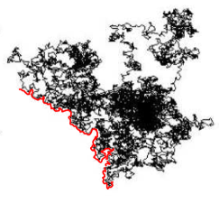
Figure 14: A Brownian path, with part of the frontier highlighted

To put this result in perspective, notice that it is rather difficult to show even that the dimension of the Brownian frontier is more than one [BJPP], and that the set of cutpoints is non-empty, [Bu]. It should also be mentioned that by work of Lawler, the intersection exponents for simple random walk are the same as for Brownian motion, so that Theorem 3.4 also shows, for instance, that

$${\mathbb{P}}[S^{1}[0,n]\cap S^{2}[0,n]=\emptyset]=\left(\frac{1}{n}\right)^{\frac{5}{8}+o(1)}$$

if $S_{1}$ and $S_{2}$ are two independent planar simple random walks started at different points.

Meanwhile, there is a more elegant approach to these dimension results, also due to Lawler, Schramm and Werner, see Section 3.3.5

3.3.3 Path properties

I have been fortunate to collaborate with Oded on several projects over the past two decades. Sometimes this meant just trying to catch up with his fast output, and watching in awe how one clever idea replaced another. But perhaps even more impressively, Oded had an amazing ability and willingness to listen, and to think along. Sometimes, when I failed in an attempt to articulate a vague idea and was about to give up a faint line of thought, he surprised me by completely understanding what I tried to express, and by continuing the thought, almost like mind reading.

The definition of $SLE_{\kappa}$ as a family of conformal maps $g_{t}$ through a stochastic differential equation does not shed much light upon the structure of the hulls $K_{t}=g_{t}^{-1}({\mathbb{H}}).$ By Section 3.3.1, it is enough to consider chordal SLE. We say that the hull $(K_{t})_{t\geq 0}$ is generated by a curve $\gamma$ if $\gamma:[0,\infty)\to\overline{\mathbb{H}}$ is continuous and if $K_{t}$ is obtained from $\gamma$ by “filling in the holes” of $\gamma[0,t]$ (more precisely, $K_{t}$ is the complement in ${\mathbb{H}}$ of the unbounded connected component of ${\mathbb{H}}\setminus\gamma[0,t]$). Since continuity of the driving term $W_{t}$ is equivalent to the requirement that the increments $K_{t+\varepsilon}\setminus K_{t}$ have “small diameter within $D_{t}$” (more precisely, there is a set $S\subset D_{t}$ of small diameter that disconnects $K_{t+\varepsilon}\setminus K_{t}$ from $\infty$ within $D_{t}$, see [LSW2], Theorem 2.6), such a curve cannot cross itself, but it can have double points and “bounce off” itself ([Po1]). There are examples of continuous $W$ for which $K_{t}$ is not locally connected, and such sets cannot be generated by curves [MR]. Fortunately, this does not happen for SLE:

Theorem 3.6 ([RoS], Theorem 5.1; [LSW9], Theorem 4.7).

For each $\kappa>0,$ the hulls $K_{t}$ are generated by a curve, almost surely.

It follows that, a.s., the conformal maps $f_{t}=g_{t}^{-1}$ extend continuously to the closed half space $\overline{\mathbb{H}}$, and ${\gamma}(t)=f_{t}(W_{t}).$ For $\kappa\neq 8$, the proof hinges on estimates for the derivative expectations ${\mathbb{E}}[|f_{t}^{\prime}(z)|^{p}]$. For $\kappa=8$, the only known proof is by exploiting the fact that $SLE_{8}$ is the scaling limit of UST, and that the UST scaling limit is a continuous curve a.s., [LSW9].

As Oded already noticed in [S9], the $SLE_{\kappa}$ trace has different phases, depending on the value of $\kappa.$

Theorem 3.7 ([RoS]).

For $\kappa\leq 4,$ the SLE trace $\gamma$ is a simple curve in ${\mathbb{H}}\cup\{0\}$, almost surely. It “swallows” points (for fixed $z\in\overline{\mathbb{H}}\setminus\{0\}$, a.s. $z\in K_{t}$ for large $t$, but $z\notin\gamma[0,\infty)$) if $4<\kappa<8$, and it is space-filling ($\gamma[0,\infty)=\overline{\mathbb{H}}$) if $\kappa\geq 8$. For all $\kappa,$ the trace is transient a.s.: $|{\gamma}(t)|\to\infty$ as $t\to\infty.$

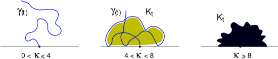
Figure 15: The three phases of SLE; picture courtesy of Michel Bauer and Denis Bernard [BB1]

Let us explain the phase transition at $\kappa=4$, already observed and conjectured in [S9] (in the radial case). Let $x>0$ and denote

$$X_{t}=g_{t}(x)-W_{t},$$

where $W_{t}=\sqrt{\kappa}B_{t}.$ Then

$$dX_{t}=\frac{2}{X_{t}}dt-\sqrt{\kappa}dB_{t}$$

is an Ito diffusion and can be easily analyzed using stochastic calculus. In fact, $X_{t}$ is a Bessel process of dimension $1+4/\kappa$. Thus $X_{t}>0$ for all $t$ if and only if $\kappa\leq 4.$ In this range, we obtain $K_{t}\cap{\mathbb{R}}=\{0\}$ for all $t,$ and it is an easy consequence of Theorem 3.6 that ${\gamma}$ is simple (if $r<s<t$ are such that ${\gamma}(r)={\gamma}(t)\neq{\gamma}(s)$, then the curve $g_{s}(\gamma[s,t])$ has the law of $SLE_{\kappa}$ shifted by $g_{s}(\gamma(s))$, but has two points on ${\mathbb{R}}$).

The other phase transition can be seen by examining the SLE-version of Cardy’s formula: If $X=\inf\bigl{(}[1,\infty)\cap\gamma[0,\infty)\bigr{)}$ denotes the first intersection of the SLE trace with the interval $[1,\infty),$ then a.s. $X=1$ if $\kappa\geq 8$, whereas for $\kappa\in(4,8)$

$${\mathbb{P}}[X\geq s]=\frac{4^{(\kappa-4)/\kappa}\,\sqrt{\pi}\,{}_{2}F_{1}(1-4/\kappa,2-8/\kappa,2-4/\kappa,1/s)\,s^{(4-\kappa)/\kappa}}{\Gamma(2-4/\kappa)\,\Gamma(4/\kappa-1/2)}\,,$$ (6)

where ${}_{2}F_{1}$ denotes the hypergeometric function. At the corresponding time where $\gamma(t)=X,$ the nontrivial interval $[1,X]$ gets “swallowed” by $K$ at once. The proof of Cardy’s formula in [RoS] is similar to the more elaborate Theorem 3.2 in [LSW2] and based on computing exit probabilities of a renormalized version of $g_{t},$

$$Y_{t}=\frac{g_{t}(1)-W_{t}}{g_{t}(s)-W_{t}}\in(0,1).$$

At the exit time $T$, we have $Y_{T}=0$ or $1$ according to whether $X<s$ or $>s.$ Now Cardy’s formula can be obtained using standard methods of stochastic calculus.

For a simply connected domain $D\neq{\mathbb{C}}$ and boundary points $p,q$, chordal SLE from $p$ to $q$ in $D$ is defined as the image of $SLE$ in ${\mathbb{H}}$ under a conformal map of ${\mathbb{H}}$ onto $D$ that takes $0$ and $\infty$ to $p$ and $q$. Since the conformal map between ${\mathbb{H}}$ and $D$ generally does not extend to $\overline{\mathbb{H}}$, the continuity of the SLE trace in $D$ does not follow from Theorem 3.6. However, using Theorem 3.9 below and general properties of conformal maps, it can be shown to still hold true, [GRS]. Another natural question is whether SLE is reversible, namely if SLE in $D$ from $p$ to $q$ has the same law as SLE from $q$ to $p.$ This question was recently answered positively for $\kappa\leq 4$ by Dapeng Zhang [Z1]. It is known to be false for $\kappa\geq 8$ [RoS], and unknown for $4<\kappa<8.$

Theorem 3.8 ([Z1]).

For each $\kappa<4,$ $SLE_{\kappa}$ is reversible, and for $\kappa\geq 8$ it is not reversible.

The aforementioned derivative expectations ${\mathbb{E}}[|f_{t}^{\prime}(z)|^{p}]$ also led to upper bounds for the dimensions of the trace and the frontier. The technically more difficult lower bounds were proved by Vincent Beffara [Be] for the trace.

For $\kappa>4$, notice that the outer boundary of $K_{t}$ is a simple curve joining two points on the real line. There is a relation between $SLE_{\kappa}$ and $SLE_{{\bf 1}6/\kappa}$, first derived by Duplantier with mathematically non-rigorous methods, and recently proved in the papers of Zhang [Z2] and Dubedat [Dub3]. Roughly speaking, Duplantier duality says that this curve is $SLE_{{\bf 1}6/\kappa}$ between the two points. A precise formulation is based on a generalization of $SLE$, the so-called $SLE(\kappa,\rho)$ introduced in [LSW8]. As a consequence, the dimension of the frontier can thus be obtained from the dimension of the dual SLE.

Based on a clever construction of a certain martingale, in [SZ] Oded and Wang Zhou determined the size of the intersection of the trace with the real line. The same result was found independently and with a different method by Alberts and Sheffield [AlSh]. Summarizing:

Theorem 3.9.

For $\kappa\leq 8,$

$$\rm{dim}\ {\gamma}[0,t]=1+\frac{\kappa}{8}.$$

For $\kappa>4,$

$$\rm{dim}\ \partial K_{t}=1+\frac{2}{\kappa}.$$

For $4<\kappa<8,$

$$\rm{dim}\ {\gamma}[0,t]\cap{\mathbb{R}}=2-\frac{8}{\kappa}.$$

The paper [SZ] also examined the question how the SLE trace tends to infinity. Oded and Zhou showed that for $\kappa<4$, almost surely ${\gamma}$ eventually stays above the graph of the function $x\mapsto x(\log x)^{-\beta},$ where $\beta=1/(8/\kappa-2).$

3.3.4 Discrete processes converging to SLE

In [LSW2], Lawler, Schramm and Werner wrote that

… at present, a proof of the conjecture that $SLE_{6}$ is the scaling limit of critical percolation cluster boundaries seems out of reach…

Smirnov’s proof [Sm1] of this conjecture came as a surprise. More precisely, he proved convergence of the critical site percolation exploration path on the triangular lattice (see Figure 12) to $SLE_{6}$. See also [CN] and [Sm2]. This result was the first instance of a statistical physics model proved to converge to an SLE. The key to Smirnov’s theorem is a version of Cardy’s formula. Lennart Carleson realized that Cardy’s formula assumes a very simple form when viewed in the appropriate geometry: When $\kappa=6,$ the right hand side $f(s)$ of (6) is a conformal map of the upper half plane onto an equilateral triangle $ABC$ such that $0,1$ and $\infty$ correspond to $A,B$ and $C.$ Since $SLE_{6}$ in $ABC$ from $A$ to $B$ has the same law as the image of $SLE_{6}$ in ${\mathbb{H}}$ from $0$ to $\infty,$ the first point $X^{\prime}$ of intersection with $BC$ has the law of $f(X).$ It follows that $X^{\prime}$ is uniformly distributed on $BC.$ (A similar statement is true for all $4<\kappa<8$, where “equilateral” is replaced by “isosceles”, and the angle of the triangle depends on $\kappa$, [Dub1]). Smirnov proved that the law of a corresponding observable on the lattice converges to a harmonic function, as the lattice size tends to zero. And he was able to identify the limit, through its boundary values. The proof makes use of the symmetries of the triangular lattice, and does not work on other lattices such as the square grid, where convergence is still unknown.

The next result concerning convergence to SLE was obtained by the usual suspects Lawler, Schramm and Werner [LSW9]. They proved Oded’s original Conjecture 3.2.2 about convergence of LERW to $SLE_{2}$, and the dual result (also conjectured in [S9]) that the UST converges to $SLE_{8}$, see Figures 10 and 13.

The harmonic explorer is a (random) interface defined as follows: Given a planar simply connected domain with two marked boundary points that partition the boundary into black and white hexagons, color all hexagons in the interior of the domain grey, see Figure 16 (a).

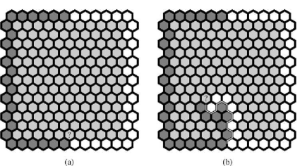
Figure 16: Definition of the Harmonic explorer path, from [SS1].

The (growing) interface $\gamma$ starts at one of the marked boundary points and keeps the black hexagons on its left and the white hexagons on its right. It is (uniquely) determined (by turning left at white hegagons and right at black) until a grey hexagon is met. When it meets a grey hexagon $h$ (marked by ? in Figure 16) the (random) color of $h$ is determined as follows. A random walk on the set of hexagons is started, beginning with the hexagon $h$. The walk stops as soon as it meets a white or black hexagon, and $h$ assumes that color. Continuing in this fashion, $\gamma$ will eventually reach the other boundary point. In [SS1], Oded and Scott Sheffield showed (distributional) convergence of $\gamma$ to $SLE_{4}$.

Figure 17: Harmonic explorer path, from [S11].

The overall strategy is again to directly analyze the Loewner driving term of the discrete path. The crucial property of $SLE_{4}$ is that, conditioned on the $SLE$ trace $\gamma[0,t]$, the probability that a point $z\in{\mathbb{H}}$ will end up on the left of $\gamma[0,\infty)$ is a harmonic function of $z$ (it is equal to the argument of $g_{t}(z)-W_{t}$, divided by $\pi$).

Other processes are believed to converge to $SLE_{4},$ too, in particular Rick Kenyon’s double domino path, and the $q-$state Pott’s model with $q=4.$

The self-avoiding walk, first proposed in 1949 as a simple model for the structure of polymers, has played an important role in the development of SLE, in several ways: First, Lawler’s invention of the LERW was partly motivated by the desire to create a model that is simpler than SAW. Second, the apparent similarity to the Brownian frontier motivated Mandelbrot’s conjecture. Third, and most significantly, the SAW is conjectured to converge to $SLE_{8/3}.$ See [LSW10] for precise formulations, and a proof of this conjecture assuming existence and conformal invariance of the scaling limit, and [K] for strong numerical evidence. However, still very little is known rigorously about the SAW.

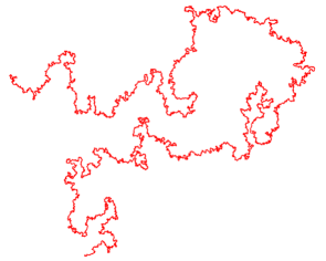
Figure 18: half-plane SAW, picture courtesy of Tom Kennedy.

Another famous classical model is the Ising model for ferromagnetism. Stas Smirnov [Sm3] has recently obtained another breakthrough concerning convergence of lattice models to SLE. He found observables for the Ising model at criticality and was able to prove their conformal invariance in the scaling limit. As a consequence, he obtained $SLE_{3}$ in the limit. Quoting from [Sm2]:

Theorem. As the lattice step goes to zero, interfaces in Ising and Ising random cluster models on the square lattice at critical temperature converge to SLE(3) and SLE(16/3) correspondingly.

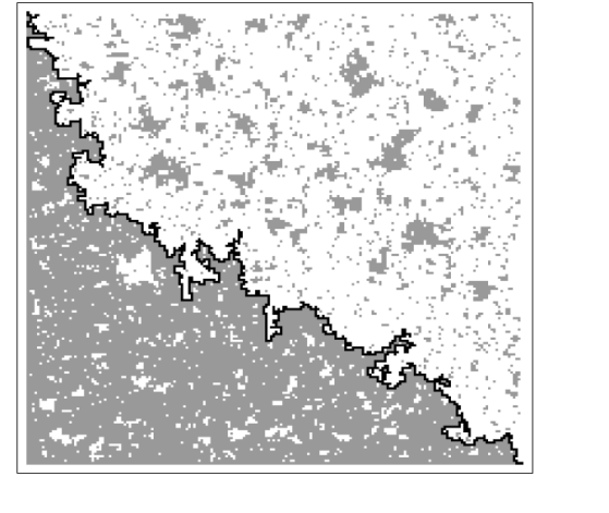
Figure 19: Critical Ising interface, picture courtesy of Stas Smirnov [Sm2].

3.3.5 Restriction measures

The elegant and important paper [LSW8] is a culmination of the universality arguments that have been initiated in [LW2] and developed in the subsequent collaboration of Lawler, Schramm and Werner. In the setting of random sets joining two boundary points of a simply connected domain, [LSW8] gives a complete characterization of laws satisfying the conformal restriction property, and various constructions of them.

Roughly speaking, a family of random sets $K$ joining 0 and $\infty$ in ${\mathbb{H}}$ satisfies conformal restriction, if for every reasonable subdomain $D={\mathbb{H}}\setminus A$ of ${\mathbb{H}}$, the law of $K$ conditioned on $K\subset D$ is the same as the law of $g(K),$ where $g$ is a conformal map from $D$ to ${\mathbb{H}}$ fixing $0$ and $\infty.$ More precisely, the sets $K$ are supposed to be connected, have connected complement, and are such that ${\mathbb{H}}\setminus K$ has two connected components. The subdomain $D$ is reasonable if it is simply connected and contains (relative) neighborhoods of $0$ and $\infty$.

An equivalent definition is to consider, for each simply connected domain $D$ and each pair of boundary points $a,b$, a law $P_{D,a,b}$ on subsets of $D$ joining $a$ and $b.$ Then the two required properties are conformal invariance, namely

$$g_{*}P_{D,a,b}=P_{g(D),g(a),g(b)}$$

for conformal maps $g$ of $D$, and “restriction”: For reasonable $D^{\prime}\subset D,$ the law $P_{D,a,b}$ of $K$, when restricted to $K\subset D^{\prime}$, equals $P_{D^{\prime},a,b}$. The remarkable main result is that there is a unique one-parameter family of such measures.

Theorem 3.10.

${\mathbb{P}}=P_{{\mathbb{H}},0,\infty}$ is a conformal restriction measure if and only if there is $\alpha>0$ such that

$${\mathbb{P}}[K\subset D]=g_{D}^{\prime}(0)^{\alpha}$$ (7)

for every reasonable $D\subset{\mathbb{H}}.$ For each $\alpha\geq\frac{5}{8}$ there is a conformal restriction measure $P_{\alpha}$. Furthermore, $\alpha_{0}=\frac{5}{8}$ is the smallest $\alpha$ for which there is a restriction measure, $P_{5/8}$ is the only restriction measure supported on simple curves, and $P_{5/8}$ is $SLE_{8/3}.$

An important observation, due to Balint Virag [V], is that $P_{1}$ is the law of Brownian excursions from $0$ to $\infty$ in ${\mathbb{H}}$ (roughly, Brownian motion started at $0$ and conditioned to “stay in ${\mathbb{H}}$” for all time). An elegant application goes as follows. If $K_{1}$ and $K_{2}$ are independent samples from $P_{\alpha_{1}}$ and $P_{\alpha_{2}}$, then (7) implies that $K_{1}\cup K_{2}$ has the law of $P_{\alpha_{1}+\alpha_{2}}$ (after the “loops” of the union have been filled in ). By uniqueness, it follows that the law of the union of 5 independent Brownian excursions in ${\mathbb{H}}$ (plus loops) is the same as that of 8 copies of $SLE_{8/3}$ (with loops added). In particular, the frontiers are the same and thus have Hausdorff dimension $4/3$ by Theorem 3.9. A similar result is [LSW8], Theorem 9.1: The law of the hull of whole-plane $SLE_{6}$, stopped when reaching the boundary of a disc $D$, is the same as the law of a planar Brownian motion (with the bounded complementary components added), stopped upon leaving $D.$

The proof that $SLE_{8/3}$ is $P_{5/8}$ is based on the following computation. Using the same notation as (5), one can show

$$d\ h_{t}^{\prime}(W_{t})=h_{t}^{\prime\prime}(W_{t})dW_{t}+\Bigl{(}\frac{h_{t}^{\prime\prime}(W_{t})^{2}}{2h_{t}^{\prime}(W_{t})}+\bigl{(}\frac{\kappa}{2}-\frac{4}{3}\bigr{)}h_{t}^{\prime\prime\prime}(W_{t})\Bigr{)}dt.$$ (8)

For $\kappa=\frac{8}{3},$ it follows that

$$d\ h_{t}^{\prime}(W_{t})^{5/8}=\frac{5}{8}\frac{h_{t}^{\prime\prime}(W_{t})}{h_{t}^{\prime}(W_{t})^{3/8}}dW_{t}$$

so that $h_{t}^{\prime}(W_{t})^{5/8}$ is a local martingale. Writing as before $T=\inf\{t:K_{t}\cap A\neq\emptyset\}$, it is not hard to show that $h_{t}^{\prime}(W_{t})$ tends to 0 as $t\to T$ if $K\cap A\neq\emptyset$ (the case $T<\infty$), and $\lim_{t\to T}h_{t}^{\prime}(W_{t})\to 1$ otherwise. Thus

$${\mathbb{P}}[K\subset D]={\mathbb{P}}[T=\infty]={\mathbb{E}}[h_{T}^{\prime}(W_{T})^{5/8}]={\mathbb{E}}[h_{0}^{\prime}(W_{0})^{5/8}]=g_{D}^{\prime}(0)^{5/8}.$$

For values greater than $5/8,$ there are several constructions of the restriction measures described in [LSW8]. One is by adding “Brownian bubbles” to SLE-traces.

3.3.6 Other results

There are other versions of the Loewner equation. The “whole plane” equation was developed and used in [LSW3] to deal with hulls $K_{t}$ that are growing in the plane rather than a disc or half-plane. “Di-polar SLE” was introduced in [BB2], see also [BBH]. An important generalization of SLE are the $SLE(\kappa,\rho)$ and variations, first introduced in [LSW8]. An elegant and unified treatment of all these variants is in [SWi]. Also, defining SLE in multiply connected domains creates a new difficulty that is not present in the simply connected case, since a slit multiply connected domain is not conformally equivalent to the unslit domain. See [Z],[BF1],[BF2].

Since SLE is amenable to computations, the convergence of discrete processes to SLE can be used to obtain results about the original process. In this fashion, Oded [S10] obtained the limiting probability, as the lattice size tends to zero in critical site percolation on the triangular lattice in the disc ${\mathbb{D}}$, that the union of a given arc $A\subset\partial{\mathbb{D}}$ and a percolation cluster surrounds $0$. In [LSW4], Lawler, Schramm and Werner showed that the probability of the event $0\leftrightarrow C_{R}$ that the percolation cluster containing the origin reaches the circle of radius $R$ behaves like $R^{-5/48},$

$$P[0\leftrightarrow C_{R}]=R^{-5/48+o(1)}$$

as $R\to\infty.$ See also [SW] for related exponents.

Because of space, in this note we have ignored the mathematically nutritious “Brownian loop soup” [LW3] and its relation to restriction measures, as well as the growing literature around the important Conformal Loop Ensemble $CLE_{\kappa}$ introduced by Scott Sheffield [Sh2]. See [W3] and [SSW].

There are deep and exciting connections between the Gaussian Free Field and SLE, as explored by Oded and Scott Sheffield. The GFF has made its first appearance in this area in Rick Kenyon’s work on the height of domino tilings [Ke3]. See [Sh1] for definitions and properties. Here is a very brief description of their work. Let $D\subset{\mathbb{C}}$ be a domain bounded by a simple closed curve that is partitioned into two arcs by two marked boundary points. Approximate $D$ by a portion $G=(V,E)$ of the triangular grid as before (see Figure 20, where again vertices are represented by hexagons), and denote $\partial V$ the boundary vertices. Fix a constant $\lambda$, and let $h=h_{\varepsilon}$ be an instance of the Discrete Gaussian Free Field, with boundary values $\pm\lambda$ on the two boundary arcs. This means that $h(v),v\in V\setminus\partial V$, is a $\sharp(V\setminus\partial V)$-dimensional Gaussian random variable whose density is proportional to $\exp(-\sum_{(u,v)\in E}(h(v)-h(u))^{2}/2).$ Extend $h$ in a piecewise linear fashion from the vertices to the triangles. The main result of the deep and very long paper [SS2] is, roughly speaking, the following. If $\lambda=3^{-1/4}\sqrt{\pi/8},$ then the level curve $\gamma_{\epsilon}$ of level $h=0$, joining the two marked boundary points, converges to $SLE_{4}$ as $\varepsilon\to 0.$ Other values of $\lambda$ lead to variants of $SLE_{4}.$ See also [SS3] and [Dub4].

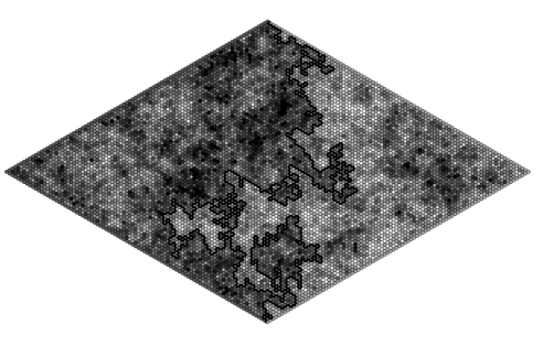
Figure 20: Level set of the Discrete GFF, from [SS2].

Finally, there are several collaborations of Oded being written at the moment. For instance, there are deep results of Christophe Garban, Gabor Pete and Oded concerning near-critical percolation and its scaling limit, which is different from $SLE_{6}$, see [GPS]. The nice paper [ShWi] describes Oded’s (unpublished) proof of Watt’s formula for double crossings in critical percolation, and provides insight into Oded’s masterful use of Mathematica. Watt’s formula was first proved rigorously by Dubedat [Dub2].

3.4 Problems

Many of Oded’s papers contain open problems, some (such as [S6]) even propose a direction to tackle them. His ICM talk [S11] contains a large number of problems around SLE, and has provided the field with a sense of direction. Some additional SLE-related problems are in [RoS]. Several of his problems have been solved since their publication.

As already mentioned, the convergence of the Ising interface to $SLE_{3}$, Problem 2.5 in [S11], was proved by Smirnov. The reversability of the chordal SLE path, Problem 7.3 of [S11], has been established for $\kappa\leq 4$ by Zhang [Z1], and the method has even led to a proof of a version of Duplantier’s duality by Zhang and by Dubedat, [Z2], [Dub3]. Near-critical percolation and dynamical percolation (Sections 2.6 and 5 of [S11]) are now well-understood by [GPS] and [NW].

Spectacular progress has been made concerning the mathematical foundations of quantum gravity. Whereas the existence of an (unscaled) limit of “random triangulations of the sphere” was already established in [AnS], the important Knizhnik-Polyakov-Zamolodchikov formula (relating exponents of statistical physics models in “random geometries” to corresponding exponents in plane geometry) seemed out of reach until recently. In Section 4 of [S11], Oded wrote:

However, there is still no mathematical understanding of the KPZ formula. In fact, the author’s understanding of KPZ is too weak to even state a concrete problem.

The Problem 4.1 in [S11], to show the existence of the (weak) Gromov-Hausdorff scaling limit of the graph metric on random triangulations of the sphere, was solved in the impressive work of Le Gall [LG]. Le Gall and Paulin showed [LGP] that the limiting space is a topological sphere, almost surely. Duplantier and Sheffield [DS] described a random measure (a scaling limit of the measure $e^{ch_{\varepsilon}}dxdy$ where $h_{\varepsilon}$ is the Gaussian free field, averaged over circles of radius $\varepsilon$) which exhibits a KPZ-like relation. They conjecture a precise relation between a scaling limit of [AnS] and their random continuous space, and discuss connections to SLE. Following Duplantier and Sheffield, simpler random metric spaces exhibiting KPZ were considered in [BS4] and [RV].

3.5 Conclusion

We have seen how Oded shaped the field of circle packings, and how he developed a deep understanding of discrete approximations to conformal maps. His results on the Koebe conjecture are still the best to date. We have also seen how Oded’s discovery of SLE led to a powerful new tool in probability theory and in mathematical physics. In fact, it has changed the way physicists and mathematicians think about critical lattice interfaces, and has led to very fruitful interactions across disciplines. The number of mathematicians and physicists working with SLE is increasing fast, and the last few years have seen a number of exciting developments. Oded has already established his place in the history of mathematics. I have no doubt that we will see many more wonderful developments directly or indirectly related to Oded’s work, thus keeping his spirit alive through the work of his fellow mathematicians, coauthors, and friends.

(a) LERW, $\kappa=2$

(b) SAW, $\kappa=\frac{8}{3}$?

(c) Ising, $\kappa=3$

(d) Harmonic explorer, $\kappa=4$

(e) Percolation, $\kappa=6$

(f) UST, $\kappa=8$

Figure 21: Various random curves converging to SLE’s

References

- [AB] M. Aizenman, A. Burchard, Hölder regularity and dimension bounds for random curves, Duke Math. J. 99 (1999), 419–453.
- [AlSh] T. Alberts, S. Sheffield, Hausdorff Dimension of the SLE curve intersected with the real line, Electron. J. Probab. 13 (2008), 1166–1188.
- [A1] E. Andreev, Convex polyhedra in Lobacevskii space, Math. USSR Sbornik 10 (1970), 413–440.
- [A2] E. Andreev, Convex polyhedra of finite volume in Lobacevskii space, Math. USSR Sbornik 12 (1970), 255-259.
- [AnS] O. Angel, O. Schramm, Uniform Infinite Planar Triangulations, Comm.Math.Phys. 241 (2003), 191–213.
- [BB1] M. Bauer, D. Bernard, Conformal Field Theories of Stochastic Loewner Evolutions, Commun. Math. Phys. 239 (2003), 493–521.
- [BB2] M. Bauer, D. Bernard, SLE, CFT and zig-zag probabilities, arXiv:math-ph/0401019v1.
- [BB3] M. Bauer, D. Bernard, 2D growth processes: SLE and Loewner chains, Phys. Rept. 432 (2006), 115–221.
- [BBH] M. Bauer, D. Bernard, J. Houdayer, Dipolar stochastic Loewner evolutions, J. Stat. Mech. Theory Exp. 3 (2005).
- [BF1] R. Bauer, R. Friedrich, Stochastic Loewner evolution in multiply connected domains, C. R. Math. Acad. Sci. Paris 339 (2004), 579–584.
- [BF2] R. Bauer, R. Friedrich, Chordal and bilateral SLE in multiply connected domains, Math. Z. 258 (2008), 241–265.
- [BSt1] A. Beardon, K. Stephenson, Circle packings in different geometries, Tohoku Math. J. 43 (1991), 27–36.
- [BSt2] A. Beardon, K. Stephenson, The Schwarz-Pick lemma for circle packings, Illinois J. Math. 35 (1991), 577–606.
- [Be] V. Beffara, The dimension of the SLE curves, Ann. Probab. 36 (2008) 1421 -1452.
- [BS1] I. Benjamini, O. Schramm, Random walks and harmonic functions on infinite planar graphs using square tilings, Ann. Probab. 24 (1996), 1219–1238.
- [BS2] I. Benjamini, O. Schramm, Harmonic functions on planar and almost planar graphs and manifolds, via circle packings, Invent. Math. 126 (1996), 565–587.
- [BS3] I. Benjamini, O. Schramm, Recurrence of Distributional Limits of Finite Planar Graphs, Electron. J. Probab. 6 (2001), 1–13.
- [BS4] I. Benjamini, O. Schramm, KPZ in one dimensional random geometry of multiplicative cascades, Comm. Math. Phys. 289 (2009), 653–662.
- [BLPS] I. Benjamini, R. Lyons, Y. Peres, O. Schramm, Uniform spanning forests, Ann. Probab. 29 (2001), 1–65.
- [BJPP] C. Bishop, P. Jones, R. Pemantle, Y. Peres, The dimension of the Brownian frontier is greater than 1, J. Funct. Anal. 143, (1997),309 336.
- [BHS] A. Bobenko, T. Hoffmann, B. Springborn, Minimal surfaces from circle patterns: geometry from combinatorics, Ann. of Math. 164 (2006), 231–264.
- [BK] M. Bonk, B. Kleiner, Quasisymmetric parametrizations of two-dimensional metric spheres, Invent. Math. 150 (2002), 127–183.
- [Bo] M. Bonk, Quasiconformal geometry of fractals, International Congress of Mathematicians. Vol. II, Eur. Math. Soc., Z”urich (2006), 1349–1373.
- [Br] M. Brandt, Ein Abbildungssatz fuer endlich-vielfach zusammenhängende Gebiete, Bull. de la Soc. des Sc. et des Lettr. de Lodz XXX, 4 (1980).
- [BSST] R. Brooks, C. Smith, A. Stone, W. Tutte, The dissection of squares into squares, Duke Math. J. 7 (1940), 312–340.
- [Bu] K. Burdzy, Cut points on Brownian paths, Ann. Probab. 17 (1989), 1012–1036.
- [CN] F. Camia, C. Newman, Critical percolation exploration path and : a proof of convergence, Probab. Theory Related Fields 139 (2007), 473 -519.
- [Can] J. Cannon, The combinatorial Riemann mapping theorem, Acta Math. 173 (1994), 155–234.
- [CFP1] J. Cannon, W. Floyd, W. Parry, Squaring rectangles: The finite Riemann mapping theorem, Contemp. Math. 169 (1994), Amer. Math. Soc., Providence, RI, 133–212.
- [CFP2] J. Cannon, W. Floyd, W. Parry, The Length-Area method and discrete Riemann mappings, manuscript (1999)
- [Car1] J. Cardy, Critical percolation in finite geometries, J. Phys. A 25(4) (1992), 201–206.
- [Car2] J. Cardy, SLE for theoretical physicists, Annals Phys. 318 (2005), 81 -118.
- [CM] L. Carleson, N. Makarov, Aggregation in the plane and Löwner’s equation, Comm. Math. Phys. 216 (2001) 583–607.
- [CMS] R. Courant, B. Manel, M. Shiffman, A general theorem on conformal mapping of multiply connected domains, Proc. Nat. Acad. Sci. U. S. A. 26 (1940), 503–507.
- [dV1] C. de Verdière, Empilements de cercles: Convergence d’une méthode de point fixe, Forum Math. I (1989), 395–402.
- [dV2] C. de Verdière, Une principe variationnel pour les empilements de cercles, Invent. Math. 104 (1991), 655–669.
- [DHR] P. Doyle, Z.-X. He, B. Rodin, Second derivatives of circle packings and conformal mappings, Discrete Comput. Geom. 11 (1994), 35–49.
- [Dub1] J. Dubedat, SLE and triangles, Elect. Comm. in Probab. 8 (2003), 28–42.
- [Dub2] J. Dubedat, Excursion decompositions for SLE and Watts crossing formula, Probab. Theory Related Fields 134 (2006), 453 -488.
- [Dub3] J. Dubedat, Duality of Schramm-Loewner Evolutions, Ann. Sci. c. Norm. Sup r. 42 (2009), 697–724.
- [Dub4] J. Dubedat, SLE and the free field: partition functions and couplings, J. Amer. Math. Soc. 22 (2009), 995–1054.
- [Duf] R. Duffin, The extremal length of a network, J. Math. Anal. Appl. 5 (1962), 200–215.
- [Dup] B. Duplantier, Conformal Random Geometry, arXiv:math-ph/0608053v1.
- [DK] B. Duplantier, K. Kwon, Conformal invariance and intersection of random walks, Phys. Rev. Let. 61 (1988), 2514–2517.
- [DS] B. Duplantier, S. Sheffield, Liouville Quantum Gravity and KPZ, arXiv:0808.1560v1.
- [Dur] P. Duren, Univalent functions, Springer-Verlag, New York, 1983.
- [GPS] C. Garban, G. Pete, O. Schramm, The scaling limit of the Minimal Spanning Tree - a preliminary report, arXiv:0909.3138.
- [GRS] C. Garban, S. Rohde, O. Schramm, Continuity of the SLE trace in simply connected domains, arXiv:0810.4327, Israel J. Math to appear.
- [GM] J. Garnett, D. Marshall, Harmonic measure, Cambridge University Press, New York, 2005.
- [GK] I. Gruzberg, L. Kadanoff, The Loewner equation: maps and shapes, J. Stat. Phys. 114 (2004), 1183–1198.
- [Ha] A. Harrington, Conformal mappings onto domains with arbitrarily specified boundary shapes, J. Analyse Math. 41 (1982), 39–53.
- [HL] M. Hastings, L. Levitov, Laplacian growth as one-dimensional turbulence, Physica D 116 (1998) 244–252.
- [He] Z.-X. He, An estimate for hexagonal circle packings, J. Differential Geom. 33 (1991), 395–412.
- [HR] Z.-X. He, B. Rodin, Convergence of circle packings of finite valence to Riemann mappings, Comm. Anal. Geom. 1 (1993), 31–41.
- [HS1] Z.-X. He, O. Schramm, Fixed points, Koebe uniformization and circle packings, Ann. of Math. (2) 137 (1993), 369–406.
- [HS2] Z.-X. He, O. Schramm, Rigidity of circle domains whose boundary has -finite linear measure, Invent. Math. 115 (1994), 297–310.
- [HS3] Z.-X. He, O. Schramm, Hyperbolic and parabolic packings, Discrete Comput. Geom. 14 (1995), 123–149.
- [HS3b] Z.-X. He, O. Schramm, A hyperbolicity criterion for circle packings, preprint, 1991.
- [HS4] Z.-X. He, O. Schramm, Koebe uniformization for “almost circle domains”, Amer. J. Math. 117 (1995), 653–667.
- [HS5] Z.-X. He, O. Schramm, The inverse Riemann mapping theorem for relative circle domains, Pacific J. Math. 171 (1995), 157–165.
- [HS6] Z.-X. He, O. Schramm, On the convergence of circle packings to the Riemann map, Invent. Math. 125 (1996), no. 2, 285–305.
- [HS7] Z.-X. He, O. Schramm, On the distortion of relative circle domain isomorphisms, J. Anal. Math. 73 (1997), 115–131.
- [HS8] Z.-X. He, O. Schramm, The -convergence of hexagonal disk packings to the Riemann map, Acta Math. 180 (1998), 219–245.
- [HK] J. Heinonen, P. Koskela, Definitions of quasiconformality, Invent. Math. 120 (1995), 61–79.
- [KN] W. Kager, B. Nienhuis, A Guide to Stochastic Loewner Evolution and its Applications, J. Stat. Phys. 115 (2004), 1149–1229.
- [K] T. Kennedy, Conformal invariance and stochastic Loewner evolution predictions for the 2D self-avoiding walk–Monte Carlo tests, J. Statist. Phys. 114 (2004), 51–78.
- [Ke1] R. Kenyon, Conformal invariance of domino tiling, Ann. Probab. 28 (2000), 759–795.
- [Ke2] R. Kenyon, The asymptotic determinant of the discrete Laplacian, Acta Math. 185 (2000), 239–286.
- [Ke3] R. Kenyon, Dominos and the Gaussian free field, Ann. Probab. 29 (2001), 1128–1137.
- [Ko1] P. Koebe, Ueber die Uniformisierung beliebiger analytischer Kurven (Dritte Mitteilung), Nachr. Ges. Wiss. Gött. (1908), 337-358.
- [Ko2] P. Koebe, Kontaktprobleme der Konformen Abbildung, Ber. Sächs. Akad. Wiss. Leipzig, Math.-Phys. Kl. 88 (1936), 141–164.
- [Ku] P. Kufarev, A remark on integrals of Löwner’s equation, Doklady Akad. Nauk SSSR 57 (1947), 655–656, in Russian.
- [La] G. Lawler, A self avoiding walk, Duke Math. J. 47 (1980), 655–694.
- [La2] G. Lawler, Geometric and fractal properties of Brownian motion and random walk paths in two and three dimensions, Bolyai Soc. Math. Stud. 9 (1998), 219–258.
- [La3] G. Lawler, Conformally Invariant Processes in the Plane, Mathematical Surveys and Monographs, 114. American Mathematical Society, Providence, RI, 2005.
- [LSW1] G. Lawler, O. Schramm, W. Werner, The dimension of the planar Brownian frontier is , Math. Res. Lett. 8 (2001), 401–411.
- [LSW2] G. Lawler, O. Schramm, W. Werner, Values of Brownian intersection exponents I, Half-plane exponents, Acta Math. 187 (2001), 237–273.
- [LSW3] G. Lawler, O. Schramm, W. Werner, Values of Brownian intersection exponents II, Plane exponents, Acta Math. 187 (2001), 275–308.
- [LSW4] G. Lawler, O. Schramm, W. Werner, One-arm exponent for critical 2D percolation, Electron. J. Probab. 7 (2002), 1–13.
- [LSW5] G. Lawler, O. Schramm, W. Werner, Values of Brownian intersection exponents III, Two-sided exponents, Ann. Inst. H. Poincar Probab. Statist. 38 (2002), 109–123.
- [LSW6] G. Lawler, O. Schramm, W. Werner, Sharp estimates for Brownian non-intersection probabilities, In and out of equilibrium (Mambucaba, 2000), 113–131, Progr. Probab., 51, Birkh user Boston, Boston, MA, 2002.
- [LSW7] G. Lawler, O. Schramm, W. Werner, Analyticity of intersection exponents for planar Brownian motion, Acta Math. 189 (2002), 179–201.
- [LSW8] G. Lawler, O. Schramm, W. Werner, Conformal restriction: the chordal case, J. Amer. Math. Soc. 16 (2003), 917–955.
- [LSW9] G. Lawler, O. Schramm, W. Werner, Conformal invariance of planar loop-erased random walks and uniform spanning trees, Ann. Probab. 32 (2004), 939–995.
- [LSW10] G. Lawler, O. Schramm, W. Werner, On the scaling limit of planar self-avoiding walk, Fractal geometry and applications: a jubilee of Beno it Mandelbrot, Part 2, 339–364, Proc. Sympos. Pure Math., 72, Part 2, Amer. Math. Soc., Providence, RI, 2004.
- [LW1] G. Lawler, W. Werner, Intersection exponents for planar Brownian motion, Ann. Probab. 27 (1999) 1601–1642.
- [LW2] G. Lawler, W. Werner, Universality for conformally invariant intersection exponents, J. Europ. Math. Soc. 2 (2000) 291–328.
- [LW3] G. Lawler, W. Werner, The Brownian loop soup, Probab. Theory Related Fields 128 (2004), 565–588.
- [LG] J. Le Gall, The topological structure of scaling limits of large planar maps, Invent. Math. 169 (2007), 621–670.
- [LGP] J. Le Gall, F. Paulin, Scaling limits of bipartite planar maps are homeomorphic to the 2-sphere, Geom. Funct. Anal. 18 (2008), 893–918.
- [Lo] C. Loewner, Untersuchungen über schlichte konforme Abbildungen des Einheitskreises, I, Math. Ann. 89 (1923), 103–121.
- [Ly] R. Lyons, A bird’s-eye view of uniform spanning trees and forests, Microsurveys in discrete probability (Princeton, NJ, 1997), 135–162.
- [M] B. Mandelbrot, The beauty of fractals, Freeman 1982.
- [MR] D. Marshall, S. Rohde, The Loewner differential equation and slit mappings, J. Amer. Math. Soc. 18 (2005), 763–778.
- [MS] D. Marshall, C. Sundberg, Harmonic measure and radial projection, Trans. Amer. Math. Soc. 316 (1989), 81–95.
- [MT] G. Miller, W. Thurston, Separators in two and three dimensions, In Proceedings of the 22nd Annual ACM Symposium on Theory of Computing, pages 300 309. ACM, Baltimore, 1990.
- [NW] P. Nolin, W. Werner, Asymmetry of near-critical percolation interfaces, J. Amer. Math. Soc. 22 (2009), 797–819.
- [Pe] R. Pemantle, Choosing a spanning tree for the integer lattice uniformly, Ann. Probab. 19 (1991), 1559 – 1574.
- [Po1] C. Pommerenke, On the Loewner differential equation, Michigan Math. J. 13 (1966), 435–443.
- [Po2] C. Pommerenke, Boundary behaviour of conformal maps, Springer Verlag, Berlin Heidelberg 1992
- [Pop1] N.V. Popova, Investigation of some integrals of the equation , Novosibirsk Gos. Ped Inst Uchon. Zapiski 8 (1949), 13–26.
- [Pop2] N.V. Popova, Relations between Löwner’s equation and the equation , Izv. Akad. Nauk BSSR, Ser. Fiz.-Mat. Nauk 6 (1954), 97–98.
- [RV] R. Rhodes, V. Vargas, KPZ formula for log-infinitely divisible multifractal random measures, 2008, arXiv:math.PR/0807.1036.
- [RSu] B. Rodin, D. Sullivan, The convergence of circle packings to the Riemann mapping, J. Differential Geometry 26 (1987), 349–360.
- [RoS] S. Rohde, O. Schramm, Basic properties of SLE, Ann. Math. 161 (2005), 879–920.
- [Sa] H. Sachs, Coin graphs, polyhedra, and conformal mapping, Discrete Math. 134 (1994), 133 -138.
- [S1] O. Schramm, Combinatorially prescribed packings and applications to conformal and quasiconformal maps, Ph. D. thesis, Princeton (1990).
- [S2] O. Schramm, Rigidity of infinite (circle) packings, J. Amer. Math. Soc. 4 (1991), 127–149.
- [S3] O. Schramm, How to cage an egg, Invent. Math. 107 (1993), 543–560.
- [S4] O. Schramm, Existence and uniqueness of packings with specified combinatorics, Israel J. Math. 73 (1991), 321–341.
- [S5] O. Schramm, Square tilings with prescribed combinatorics, Israel J. Math. 84 (1993), 97–118.
- [S6] O. Schramm, Transboundary extremal length, J. Anal. Math. 66 (1995), 307–329.
- [S7] O. Schramm, Conformal uniformization and packings, Israel J. Math. 93 (1996), 399–428.
- [S8] O. Schramm, Circle patterns with the combinatorics of the square grid, Duke Math. J. 86 (1997), 347–389.
- [S9] O. Schramm, Scaling limits of loop-erased random walks and uniform spanning trees, Israel J. Math. 118 (2000), 221–288.
- [S10] O. Schramm, A percolation formula, Electron. Comm. Probab. 6 (2001), 115–120.
- [S11] O. Schramm, Conformally invariant scaling limits: an overview and a collection of problems. In Proceedings of ICM Madrid 2006, 1, 513–543. European Math. Soc. 2007.
- [SS1] O. Schramm, S. Sheffield, Harmonic explorer and its convergence to , Ann. Probab. 33 (2005), 2127–2148.
- [SS2] O. Schramm, S. Sheffield, Contour lines of the two-dimensional discrete Gaussian free field, Acta Math. 202 (2009), 21–137.
- [SS3] O. Schramm, S. Sheffield, A contour line of the continuum Gaussian free field, preprint (2010).
- [SSW] O. Schramm, S. Sheffield, D. Wilson, Conformal radii for conformal loop ensembles, Comm. Math. Phys. 288 (2009), 43–53.
- [SWi] O. Schramm, D. Wilson, SLE coordinate changes, New York J. Math. 11 (2005), 659–669.
- [SZ] O. Schramm, W. Zhou, Boundary proximity of SLE, Probab. Theory Related Fields 146 (2010), 435–450.
- [Sh1] S. Sheffield, Gaussian free fields for mathematicians, Probab. Theory Related Fields 139 (2007), 521–541.
- [Sh2] S. Sheffield, Exploration trees and conformal loop ensembles, Duke Math. J. 147 (2009), 79–129.
- [ShWi] S. Sheffield, D. Wilson, Schramm’s proof of Watts’ formula, rXiv:1003.3271.
- [Sm1] S. Smirnov, Critical percolation in the plane: conformal invariance, Cardy’s formula, scaling limits, C. R. Acad. Sci. Paris S r. I Math. 333 (2001), 239–244.
- [Sm2] S. Smirnov, Towards conformal invariance of 2D lattice models, In Proceedings of ICM Madrid 2006, 2, 1421–1451. European Math. Soc. 2007.
- [Sm3] S. Smirnov, Conformal invariance in random cluster models I, Holomorphic fermions in the Ising model, arXiv:0708.0039, Ann. Math., to appear.
- [SW] S. Smirnov, W. Werner: Critical exponents for two-dimensional percolation, Math. Rev. Lett. 8 (2001), 729 744.
- [Ste1] K. Stephenson, A probabilistic proof of Thurston’s conjecture on circle packings, Rend. Sem. Mat. Fis. Milano 66 (1996), 201–291.
- [Ste2] K. Stephenson, Introduction to circle packing. The theory of discrete analytic functions, Cambridge University Press, Cambridge, 2005.
- [Str] K. Strebel, Über das Kreisnormierungsproblem der konformen Abbildung, Ann. Acad. Sci. Fennicae. Ser. A 101 (1951), 1–22.
- [T] W. Thurston, The geometry and Topology of 3-manifolds, Chap. 13 (Math. Notes, Princeton) Princeton University Press 1980.
- [V] B. Virag, Brownian Beads, Probab. Theory Related Fields 127 (2003), 367–387.
- [W1] W. Werner, Random planar curves and Schramm-Loewner evolutions, Lecture Notes in Math. 1840, Springer, Berlin, 2004.
- [W2] W. Werner, Conformal restriction and related questions, Probab. Surv. 2 (2005), 145–190.
- [W3] W. Werner, The conformally invariant measure on self-avoiding loops, J. Amer. Math. Soc. 21 (2008), 137–169.
- [WS] T. Witten, L. Sander, Diffusion-limited aggregation, a kinetic phenomenon, Phys. Rev. Lett. 47 (1981), 1400 -1403.
- [Z] D. Zhan, Loewner evolution in doubly connected domains, Probab. Theory Related Fields 129 (2004), 340–380.
- [Z1] D. Zhan, Reversibility of chordal SLE, Ann. Probab. 36 (2008), 1472–1494.
- [Z2] D. Zhan, Duality of chordal SLE, Invent. Math. 174 (2008), 309–353.