Finite range effects in (d,p) reactions

Abstract

With the increasing interest in using (d,p) transfer reactions to extract structure and astrophysical information, it is important to evaluate the accuracy of common approximations in reaction theory. Starting from the zero-range adiabatic wave model, which takes into account deuteron breakup in the transfer process, we evaluate the importance of the finite range of the $n-p$ interaction in calculating the adiabatic deuteron wave (as in Johnson and Tandy) as well as in evaluating the transfer amplitude. Our study covers a wide variety of targets as well as a large range of beam energies. Whereas at low beam energies finite range effects are small (below 10%), we find these effects to become important at intermediate energies (20 MeV/u) calling for an exact treatment of finite range in the analysis of (d,p) reactions measured at fragmentation facilities.

I Introduction

Since the early days of nuclear physics, transfer reactions have been a preferred tool to study spectroscopic properties of nuclei and have been widely used to determine single particle structure across the nuclear chart (e.g. niewo66 ; daehnick69 ; bainum77 ; schiffer04 ). Such studies have allowed a better understanding of detailed features of nuclear interactions. It was through a systematic study of single nucleon transfer on Sn isotopes, that we now understand the reduction of the spin-orbit strength when moving toward neutron rich systems schiffer04 . One would also like to use the transfer reaction method to discriminate between effective interactions used in the shell model, as suggested in the study of (d,p) on Ni isotopes lee09 . Nowadays the spectroscopy of exotic nuclei can be studied using inverse kinematics. Pioneering studies li8dp ; he6dp ; li9dp ; ge83se85 ; Catford2005 hold promise for applying this technique more broadly, especially in new generation rare isotope facilities, where beam rates will be enhanced.

Another intriguing aspect of nuclear structure is the role of correlations. The independent particle shell model of course neglects all correlations. State-of-the-art shell model include some correlations effectively through the residual interactions. Electron knockout experiments have shown a 30% decrease in the spectroscopic factors of closed shell nuclei as compared to the independent shell model predictions, a reduction that is understood in terms of short range correlations kramer . Reduction factors from nuclear knockout experiments can be much larger, depending on the difference between the neutron and proton separation energies lee09prl . However, the physical reason for such a large suppression is still unclear, long range correlations being a possibility barbieri . What is most intriguing is that spectroscopic factors from transfer reactions show no dependence on the difference in neutron-proton separation energies. Large surveys of ground state spectroscopic factors from (d,p) reactions tsang05 , including nuclei with a wide range of separation energies (0.5-19 MeV) show good agreement with large scale shell model using modern effective interactions.

The reconciliation of these results with those from knockout experimentsgade08 is proving difficult and is the subject of recent work on new approaches to the calculation of overlap functionsTimofeyuk2009 ; barbieri . The resolution of these important physics questions relies on the accuracy of the reaction model being used. It is thus of paramount importance that the reaction theory is well founded and uncertainties are well understood. In this respect there have been a number of works looking at specific aspects of the reactions theory used for the analysis of (d,p) transfer data (uncertainties in the optical potentials liu04 , coupling to excited states of the target delaunay05 and ambiguities due to the single particle wave functions muk05 ; pang06 and new ways of calculating overlap functions Timofeyuk2009 ; barbieri ). In this work we explore another aspect: the consequences of the non-zero range of the $n-p$ interaction that plays a key role in the theory is several different ways.

Over the past four decades of work on (d,p) reactions, different approximations were made, not only regarding the optical potentials, the deuteron and final single-particle wavefunctions, but also in the reaction mechanism and the evaluation of the transfer matrix element. It may thus be confusing to realize the large range of spectroscopic factors available in the literature. Systematic and consistent studies tsang05 ; lee07 ; tsang09 ; lee09 provide a much better overall assessment of the situation. In tsang05 ; lee07 an extensive survey of ground state spectroscopic factors from charge $Z=3-24$ was performed using the same reaction model, the same global potentials and the same single particle parameters. With these same assumptions, spectroscopic factors extracted from 235 sets of (d,p) data were found consistent with shell model predictions to within $\pm 20$%. An identical study was performed on excited states tsang09 , and although there were a few unresolved cases (such as the Ni isotopes), the overall agreement with shell model was of the order of $40$%. Ni isotopes were studied separately lee09 and a better overall description of these nuclei was found with a modified effective interaction in the shell-model calculations.

All these studies rely on the adiabatic distorted-wave approximation (ADWA) developed by Johnson and Soper soper and the local energy approximation (LEA) lea to take into account the finite range of the $n-p$ interaction $V_{np}$ in evaluating the $(d,p)$ transition matrix.

In soper , a three-body theory for A(d,p)B was developed taking into account deuteron breakup which is known to be important even for reactions on stable nuclei. In soper the zero range approximation is made for the $n-p$ interaction. Then, the transfer matrix element reduces to a form similar to the zero range Distorted Wave Born Approximation (DWBA) where the scattering wavefunction in the incident channel is calculated with an adiabatic potential consisting of the sum of the proton and neutron potentials evaluated at half the deuteron energy, instead of the deuteron optical potential extracted from (d,d) data. ADWA typically decreases the radius and diffuseness of the distorting potential harvey compared with typical values for deuteron optical potentials deduced from elastic deuteron scattering and often provides a better description of the data johnson-ria .

An adiabatic theory including finite range effects was formally developed by Johnson and Tandy tandy . Using a Weinberg expansion in the deuteron channel, Johnson and Tandy arrive at a set of coupled channel equations to describe the relative motion of the centre of mass of the neutron and proton relative to the target. The solution of the coupled channels equations gives a three-body wavefunction that is a coherent superposition of the bound (deuteron) and break-up continuum states of the $n-p$ system.

In this paper we will confine ourselves to the simplest version of this theory in which only the first term in the Weinberg expansion is retained. This assumes that the only significant break-up components in the three-body wavefunction have sufficiently small energies that inside the range of $V_{np}$, the relevant $n-p$ scattering states have the same radial shape as the deuteron ground state wave function. When only the first Weinberg term is included, the coupled equations reduce to an optical-model-like equation for the three-body wavefunction where the distorting potential is the sum of the neutron and proton optical potentials multiplied by the neutron-proton interaction, folded over the deuteron bound state.The effect of other components laid have been shown to be significant at $E_{d}=88$ MeV but their effects at lower energies are unknown.

In the early sixties, it was already understood that finite range effects were important in (d,p) reactions, however due to computational limitations, all calculations were performed in zero range. A very popular procedure to correct a zero range calculation was developed by Buttle and Goldfarb lea . The standard implementation of this method, the so-called local energy approximation (LEA), takes only the first term of the expansion presented in lea . For deuteron energies well above the Coulomb barrier, it is not clear that this procedure is sufficiently accurate. A simple estimate of the modification of the Johnson and Soper potential due to a finite range $V_{np}$ were reported in wales .

In this work, we perform a systematic study of finite range effects in (d,p) reactions within the framework of ADWA. We consider 26 (d,p) reactions on stable targets, involving nuclei with masses ranging $A=12-208$ and deuteron energies $E_{d}=2-70$ MeV. We first study the finite range effects on the distorting potential potential in the incident channel following the method by Johnson and Tandy tandy . In addition, we consider finite range effects in the evaluation of the transfer matrix element and the accuracy of the LEA. We also explore the implications of our study to reactions involving loosely bound nuclei.

The paper is organized in the following way: reaction theory is revised in Sec. II, results are presented in Sec. III and further discussed in section IV. Finally, conclusions are drawn in Sec. V.

II Theory

Our starting point is a three-body model of the $n+p+A$ system, see book , Ch.7 . In this model the scattering wavefunction $\Psi^{(+)}(\vec{r},\vec{R})$ corresponding to a deuteron incident on a nucleus $A$ is the solution of the inhomogeneous differential equation

$$[E+i\epsilon-T_{\mathbf{r}}-T_{\mathbf{R}}-U_{nA} - U_{pA}-V_{np}]\Psi^{(+)}(\vec{r},\vec{R})$$ (1)

$$= \imath\epsilon\phi_{d}(\vec{r})\exp(\imath\vec{K}_{d}.\vec{R}).$$

Here $T_{\mathbf{r}}$ and $T_{\mathbf{R}}$ are the total kinetic energy operators associated with the n-p relative motion and the motion of the $n+p$ centre of mass relative to the target, where $\vec{r}=\vec{r}_{p}-\vec{r}_{n}$ and $\vec{R}=(\vec{r}_{n}+\vec{r}_{p})/2$. We take $\vec{r}_{n}$ and $\vec{r}_{p}$ to be the neutron and proton coordinates relative to the center of mass of the target $A$.

In Eq.(1) the interactions $U_{nA}(\vec{r}_{n})$, $U_{pA}(\vec{r}_{p})$ and $V_{np}(\vec{r})$ are the neutron-target, proton-target and neutron-proton interactions, respectively. The term proportional to $\imath\epsilon$ on the r.h.s. of Eq.(1) ensures that there is an incoming wave only in the deuteron channel.

One way of calculating the exact (d,p) transition amplitude, $T$, from $\Psi^{(+)}(\vec{r},\vec{R})$ is to use the formulation of Timofeyuk and Johnsontimofeyuk99 . In the limit $\epsilon\rightarrow 0$, the transition amplitude $T$ is given by:

$$T=<\phi_{nA}\tilde{\chi}^{(-)}_{pB}|V_{np}|\Psi^{(+)}>\,,$$ (2)

where $\phi_{nA}$ is the final state of the neutron-target system, and $\tilde{\chi}^{(-)}_{pB}$ has a plane wave proton and an incoming scattered wave distorted by $U_{pA}^{*}$ timofeyuk99 ; johnson09 . Note that in this formulation there is no remnant term and the proton distorted wave is generated by $U_{pA}^{*}$ not $U_{pB}^{*}$. Eq.(4) neglects recoil effects of order $1/A$ which were evaluated in timofeyuk99 . They are negligible in all the cases discussed here except possibly for ¹²C. The connection between this formulation and standard 3-body methods based on the Faddeev equations altetal is explained injohnson09 .

A more common expression for the transition amplitude for this process is:

$$T=<\phi_{nA}\chi^{(-)}_{pB}|V_{np}+U_{pA}-U_{pB}|\Psi^{(+)}>\,,$$ (3)

where $\phi_{nA}$ is the final state of the neutron-target system, and $\chi_{pB}^{(-)}$ is a proton scattering wave distorted by $U_{pB}^{*}$. In the many-body generalisation of Eq.(3) the remnant term $U_{pA}-U_{pB}$ is a function of the internal coordinates of $A$ and $B$ and makes the interpretation of the transition amplitude in terms of nuclear structure (overlap functions) much more complicated than when Eq.(2) is used. This introduces into the formulation an additional optical potential $U_{pB}$ and thus larger uncertainties into the analysis since in most applications to exotic nuclei this potential is not well determined. Many of the recent applications have used Eq.(3) and neglected the remnant term $U_{pA}-U_{pB}$:

$$T=<\phi_{nA}\chi^{(-)}_{pB}|V_{np}|\Psi^{(+)}>\,.$$ (4)

Neglecting the remnant term is a very good approximation for all cases discussed here with the exception of ¹²C. Eq.(4) is the starting point for the present study.

The important realization in soper ; tandy is that with Eq.(2) or Eq.(4), the full three-body wavefunction $\Psi^{(+)}(\vec{r},\vec{R})$ is only required within the range of the $V_{np}$ interaction. A major simplification is achieved in the limit of the zero-range approximation as then only $\Psi^{(+)}(0,\vec{R})$ is needed.

II.1 Johnson and Soper method

The method developed by Johnson and Soper soper is based on an expansion of the three-body wavefunction $\Psi^{(+)}(\vec{r},\vec{R})$ in the complete set of eigenstates of the $n-p$ Hamiltonian:

$$(T_{r}+V_{np})\phi_{d}(\vec{r}) = -\varepsilon_{d}\phi_{d}(\vec{r})\,,$$

$$(T_{r}+V_{np})\phi_{k}(\vec{r}) = +\varepsilon_{k}\phi_{k}(\vec{r})\,.$$ (5)

Here $\phi_{d}(\vec{r})$ is the deuteron wave function while scattering states are represented by $\phi_{k}(\vec{r})$. The three-body wavefunction is then expanded as:

$$\Psi^{(+)}(\vec{r},\vec{R})=\phi_{d}(\vec{r})\chi_{d}(\vec{R})+\int\mathrm{d}\vec{k}\phi^{(+)}_{k}(\vec{r})\chi_{k}(\vec{R})\;.$$ (6)

When this expansion is introduced in Eq.(1), and assuming that the excitation energies of the deuteron are small compared to the deuteron initial kinetic energy $\varepsilon_{k}+\varepsilon_{d}<<E$, the three-body equation for $r=0$ reduces to an optical model equation:

$$(E+\epsilon_{d}-T_{R}-U_{JS}(R))\chi^{JS}_{d}(\vec{R})=0\,,$$ (7)

where the effective potential $U_{JS}$ does not describe deuteron elastic scattering, but rather incorporates deuteron breakup effects within the range of $V_{np}$:

$$U_{JS}(R)=U_{nA}(R)+U_{pA}(R)\,.$$ (8)

Within this model, the transfer amplitude reduces to

$$T_{JS}=D_{0}\int\mathrm{d}R\,\phi_{nA}^{*}(\vec{R})\chi_{pB}^{*}(\vec{R}){\chi}^{JS}_{d}(\vec{R})$$ (9)

where $D_{0}$ is the zero range constant of the deuteron.

II.2 The Johnson and Tandy generalisation of the Johnson Soper method

The Johnson and Tandy tandy approach again builds on the fact that the three-body wavefunction is only needed within the range of $V_{np}$. While the continuum discretized coupled channel method (CDCC) cdcc uses a basis of eigenstates of the $n-p$ Hamiltonian which is complete for all values of the $n-p$ separation $\vec{r}$, as in Eq.(6), here the Weinberg basis is introduced:

$$(T_{r}+\alpha_{i}V_{np})\phi_{i}(\vec{r})=-\varepsilon_{i}\phi_{i}(\vec{r})$$ (10)

with $i=1,2,...$ and the orthonormality relation $\langle\phi_{i}|V_{np}|\phi_{j}\rangle=-\delta_{ij}$. The Weinberg states (or Sturmians) form a complete basis within the range of the $V_{np}$ interaction and thus they are particularly suited to describing the problem when using the transfer amplitude written as in Eq.(4). A clear advantage of this basis as compared to Eq.(6) is that it is square integrable.

The three-body wavefunction is then expanded as:

$$\Psi^{(+)}(\vec{r},\vec{R})=\sum_{i=1}^{\infty}\phi_{i}(\vec{r})\chi_{i}(\vec{R}).$$ (11)

When this expansion is introduced into the three-body equation Eq.(1), one obtains a set of coupled channel equations:

$$[E+i\epsilon-K_{\mathbf{R}}-\bar{U}_{ii}(\vec{R})]\chi_{i}(\vec{R})=$$

$$\imath\epsilon\delta_{i1}N_{d}\exp(\imath\vec{K}_{d}.\vec{R})+\sum_{j\neq i}\bar{U}_{ij}(\vec{R})\chi_{j}(\vec{R}).\,$$ (12)

The coupling potentials are defined by $\bar{U}_{ij}(\vec{R})=U_{ij}+\beta_{ij}(\alpha_{j}-1)$ and $U_{ij}(\vec{R})=-\langle\phi_{i}|V_{np}(U_{nA}+U_{pA}|\phi_{j}\rangle$ where $\beta_{ij}=\langle\phi_{i}|V^{2}_{np}|\phi_{j}\rangle$ and $\alpha_{j}$ are the eigenvalues of the Wienberg equation Eq.(10). The normalization coefficient appearing on the r.h.s of Eq.(12) is $N_{d}=-\langle\phi_{1}|V_{np}|\phi_{d}\rangle$.

These coupled channel equations can be solved exactly as done in laid but reduce to a much simpler form if only the first term of the expansion Eq.(11) is necessary. In that case, $\alpha_{1}=1$ and we can arrive at the following optical model type equation:

$$(E+\epsilon_{d}+i\varepsilon-T_{R}-U_{11}(R))\chi^{JT}_{1}(\vec{R})=i\varepsilon N_{d}\,\exp(\imath\vec{K}_{d}.\vec{R}),$$ (13)

where now the potential is still related to the sum of the proton and neutron potentials as in Johnson and Soper, but involves a more complex folding procedure:

$$U_{11}(R)=-\langle\phi_{1}(\vec{r})|V_{np}(U_{nA}+U_{pA})|\phi_{1}(\vec{r})\rangle\,.$$ (14)

Apart from the normalization, $\phi_{1}$ is the ground state wavefunction of the deuteron $\phi_{d}$. Then the potential $U_{11}(R)$ can also be written in terms of $\phi_{d}$:

$$U_{11}(R)\equiv U_{JT}(R)=\frac{\langle\phi_{d}(\vec{r})|V_{np}(U_{nA}+U_{pA})|\phi_{d}(\vec{r})\rangle}{\langle\phi_{d}(\vec{r})|V_{np}|\phi_{d}(\vec{r})\rangle}\,.$$ (15)

In this case the transfer amplitude is defined through the 6-dimensional integral:

$$T = <\phi_{nA}\chi^{(-)}_{pB}|V_{np}|\phi_{1}\chi^{JT}_{1}(\vec{R})>$$ (16)

$$= <\phi_{nA}\chi^{(-)}_{pB}|V_{np}|\phi_{d}(\chi^{JT}_{1}(\vec{R})/N_{d})>.$$

where we have used $\mid\phi_{d}\,>=N_{d}\mid\phi_{1}>$.

We see from Eq.(13) that $(\chi^{JT}_{1}(\vec{R})/N_{d})$ is a distorted wave generated by the potential $U_{11}$ and normalized to an incident wave of unit amplitude.

In the following section we will compare the cross sections obtained with Eq.(9) and Eq.(16). We also disentangle the separate effects of finite range in the potential $U_{11}$, looking specifically at the potentials from Eq.(8) and (14), and that of finite range in the evaluation of the transfer amplitude.

III Results

We perform a systematic study of finite range effects on 26 (d,p) reactions. In all our calculations we take the Reid interaction for the deuteron rsc and the Chapel Hill global parameterization for the nucleon optical potentials ch89 . In calculating the potential of Eq.15 we neglect the d-wave part of the $\phi_{d}$. For all cases here presented, the final bound single particle state is obtained using a potential with standard radius and diffuseness $r=1.2$ fm and $a=0.65$ fm and adjusting the depth to the known neutron separation energy of the corresponding final state. In Subsection(IIIA) we show our results for the potential and then present the results for the (d,p) cross sections in Subsection(IIIB).

III.1 Finite range effects in the potentials

Johnson and Tandy potentials Eq.(15) are computed, using a subroutine contained in the code TWOFNR twofnr for performing the $r$ integrations needed, and compared with the Johnson and Soper adiabatic potentials Eq.(8) for 26 cases. In order to simplify the comparison we fit the real part of the resulting $U_{JT}$ to a volume Woods Saxon shape and the corresponding imaginary to a surface Woods Saxon form. For all cases studied we find that the most important difference between the interactions $U_{JT}$ and $U_{JS}$ is a constant increase in diffuseness. There is also a slight systematic decrease in radius. Differences in the depths of the real and imaginary parts are more subtle and vary case to case. In wales , an approximate method to estimate finite range corrections to the adiabatic potential was developed. In that method, the radius is fixed but an increase in diffuseness is predicted with a decrease in the depth of the potential. In table 1 we show the percentage difference of our numerically calculated $U_{JT}$ and the Wales and Johnson approximate prescription $U_{WJ}$ wales , relative to the zero-range Johnson and Soper potential $U_{JS}$, for three reference cases. Percentage differences are calculated at the radius for which the potential is maximum.

The main feature of $U_{JT}$ compared to $U_{JS}$ is captured by the Wales and Johnson prescription, namely the increase in the diffuseness in both the real and imaginary part of the interaction. However the Wales and Johnson results differ quantitatively from ours.

Table 1: Finite range effects on the Johnson-Tandy distorting potential, Eq.(15): in the 3rd column the Wales and Johnson potential is compared with the zero range potential $U_{JS}$ and in the 4th column the Johnson and Tandy $U_{JT}$ is compared with $U_{JS}$. We compare the diffuseness of the real and imaginary parts, $a_{R}$ and $a_{I}$, as well as the depths of the real and imaginary parts $V$ and $W_{s}$, and the corresponding radii $r_{R}$ and $r_{I}$.

target	parameter	$U_{WJ}$	$U_{TJ}$
all	$a_{R}$	+4%	+7%
	$a_{I}$	+3%	+8-9%
12C	$V$	-5.6%	-1.98%
	$r_{R}$	0%	-1.25%
	$W_{s}$	-4.6%	-4.52%
	$r_{I}$	0%	+0.72%
48Ca	$V$	-2.1%	-0.04%
	$r_{R}$	0%	-0.93%
	$W_{s}$	-3.7%	+1.6%
	$r_{I}$	0%	-0.97%
208Pb	$V$	-0.7%	+0.06%
	$r_{R}$	0%	-0.35%
	$W_{s}$	-3.3%	+1.2%
	$r_{I}$	0%	-0.35%

III.2 Finite range effects in the transfer cross sections

Table 2: Percentage differences of finite range effects in (d,p) reactions relative to the zero-range Johnson and Soper calculation (* denotes cases for which no data is available). The target nucleus, the deuteron incident energy in the laboratory (in MeV) and the angle (in degrees) at which the percentage differences are evaluated are given in the 1st, 2nd and 3rd column respectively.

Target	$E_{d}$	$\theta$	$\Delta$(LEA)	$\Delta$(FR-JS)	$\Delta$(FR-JT)	$\Delta$(JT-JS)
12C	4	25	+5.6%	+5.5%	+4.5%	-1.0%
12C	12	13	+2.6%	+2.9%	-1.5%	-4.3%
12C	19.6	10	+11%	+13%	+7.7%	-4.2%
12C	56	6	-37%	-27%	-36%	-12%
48Ca	2	180	+6.5%	+6.3%	+2.6%	-3.5%
48Ca	13	12	+4.9%	+3.8%	-2.8%	-6.2%
48Ca	19	8	+5.0%	+4.0%	-0.30%	-4.1%
48Ca*	30	4		+7.3%	+4.8%	-2.3%
48Ca*	40	0		-5.4%	-5.9%	-10%
48Ca*	50	0		-1.9%	-19%	-18%
48Ca	56	0	-5.2%	-6.5%	-24%	-18.6%
69Ga	12	14	+4.3%	+4.7%	-1.1%	-5.49%
86Kr	11	25	+4.8%	+5.5%	-0.40%	-5.63%
90Zr	2.7	138	+6.2%	+7.3%	+5.5%	-1.7%
90Zr	11	26	+5.4%	+5.0%	-0.90%	-5.6%
124Sn	5.6	175	+6.1%	+11%	+7.5%	-2.8%
124Sn	33.3	0	+2.9%	+4.6%	0%	-4.4%
124Sn*	40	12		-1.1%	-2.4%	-1.4%
124Sn*	50	11		-3.9%	-4.3%	-0.44%
124Sn*	60	9		-11%	-30%	-21%
124Sn*	70	0	+5.1%	-29%	-44%	-21%
208Pb	8	180	+6.1%	+7.2%	+6.1%	-0.96%
208Pb	12	98	+5.7%	+8.8%	+2.2%	-6.1%
208Pb*	20	30		+4.5%	-2.3%	-6.6%
208Pb*	40	9		+1.4%	-6.9%	-8.1%
208Pb*	60	0		+0.14%	-8.8%	-9.0%
208Pb*	80	0		-62%	-86%	-63%

Once the adiabatic potentials are defined, cross sections can be obtained. The matrix element in Eq.(9) was evaluated using the adiabatic wavefunction distorted by $U_{JS}$ and the zero-range constant $D_{0}$ was obtained from the Reid n-p interaction rsc for consistency. The finite range calculation Eq.(16) uses $U_{JT}$ for the adiabatic wavefunction.

To assess the relative importance of the finite range effect in the adiabatic potential and that on the evaluation of the transfer amplitude, we also perform a finite range calculation using $U_{JS}$. Finally, given that the LEA method lea has been widely used in the past, we also perform a calculation where Eq.(9) is evaluated using the Johnson and Soper adiabatic potential $U_{JS}$ but making the local energy correction lea . All calculations are performed using the code fresco fresco .

In table 2 we quantify these effects for all the reactions studied. All percentage differences are calculated at the first peak of the angular distribution (with the exception of the sub-Coulomb examples for which percentage differences are calculated at backward angles) and are relative to the Johnson and Soper approach Eq.(9):

• $\Delta$(LEA) shows the effect of finite range in the evaluation of the T-matrix when the LEA is used in conjunction with the Johnson and Soper model;

• $\Delta$(FR-JS) shows the effect of finite range in the evaluation of the T-matrix when fixing the adiabatic potential to $U_{JS}$;

• $\Delta$(FR-JT) shows the full finite range effects when finite range is taken into account properly both in the evaluation of the T-matrix and the adiabatic potential ($U_{JT}$);

• $\Delta$(JS-JT) is the percentage difference between finite range calculations using $U_{JT}$ and $U_{JS}$ and therefore shows the effect of including finite range in the adiabatic potential.

In the table 2 we indicate the angle at which the percentage differences of cross sections were calculated.

In addition to the full table, we also select some angular distributions that illustrate the various trends we observed, presented in Figs.1-3. Each plot contains four lines: a dotted line corresponding to the zero-range Johnson and Soper calculation, a dashed line corresponding to the local energy correction to the $T$-matrix calculation with the Johnson and Soper potential, the long-dashed line corresponding to a full finite range $T$-matrix calculation where $U_{JS}$ is used, and the full line is a finite range $T$-matrix calculation with the finite range adiabatic potential $U_{JT}$. Data is also presented whenever available, but only as an indication that the ingredients of our model are realistic and therefore the magnitude of the finite range effects reliable. It is not the purpose of this work to extract spectroscopic information for these systems.

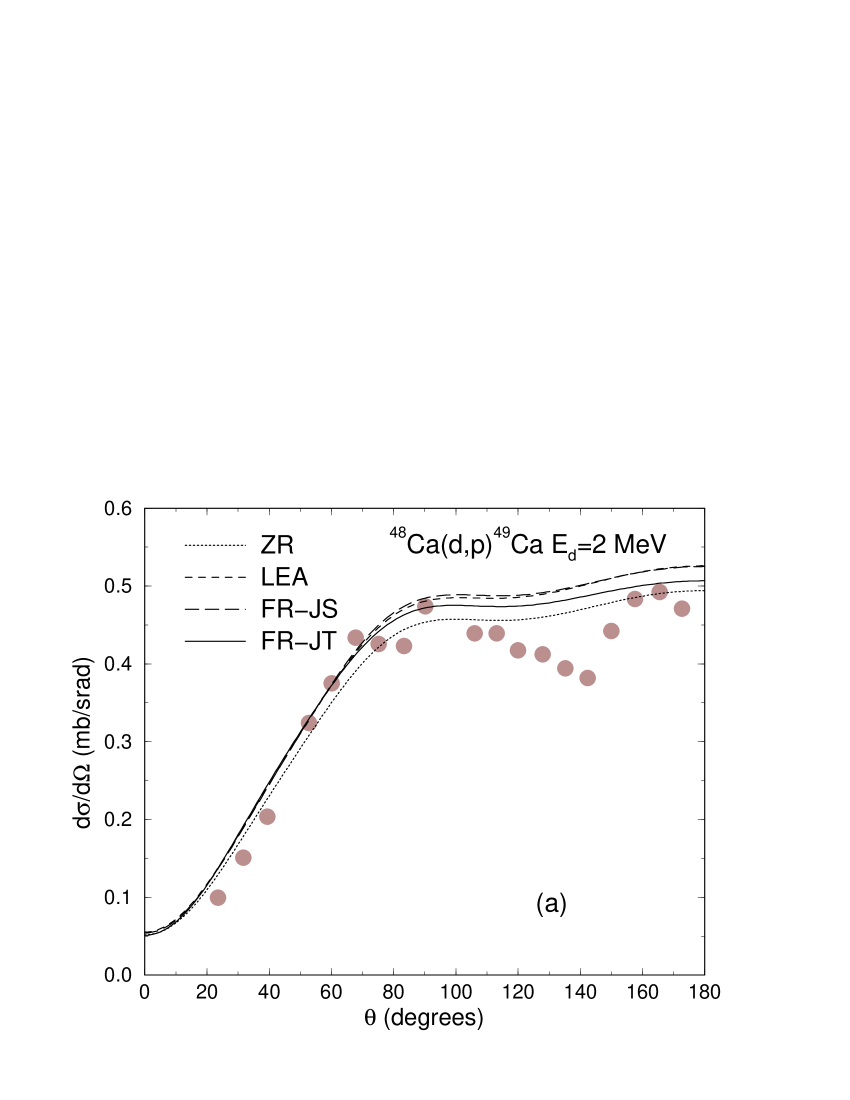
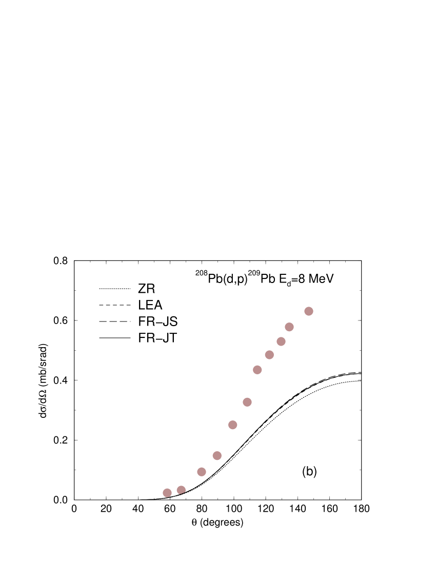
Figure 1: Angular distributions for (d,p) at sub-Coulomb energies: (a) ⁴⁸Ca(d,p)⁴⁹Ca(g.s.) $E_{d}=2$ MeV (data from ca48-2 ) and (b) ²⁰⁸Pb(d,p)²⁰⁹Pb(g.s.) $E_{d}=8$ MeV (data from pb208-8 ). Comparison of zero-range Johnson and Soper model (dotted), the LEA Johnson and Soper model (dashed), a finite range calculation of the transfer amplitude using the Johnson and Soper adiabatic wave (long-dashed) and the full finite range results (solid line).

We first look at sub-Coulomb transfer reactions, which are usually rather insensitive to the nuclear optical potential. In Fig.1(a) we show ⁴⁸Ca(d,p)⁴⁹Ca at $E_{lab}=2$ MeV and in Fig.1(b) ²⁰⁸Pb(d,p)²⁰⁹Pb at $E_{lab}=8$ MeV. In both cases, the effects of finite range are only a few percent (3% in ⁴⁸Ca and 6% in ²⁰⁸Pb), and these are mostly due to the approximation in the evaluation of the T-matrix and not from the adiabatic potential. In this case, LEA is able to capture most of the finite range effects. In the sub-Coulomb energy regime, for all cases studied, errors in using the Johnson and Soper potential with the local energy approximation are below 5%.

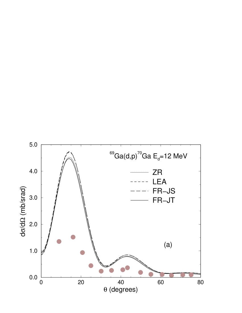
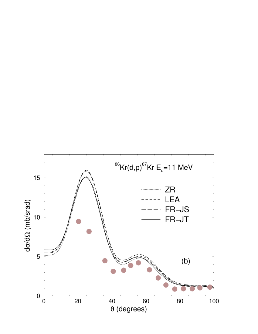
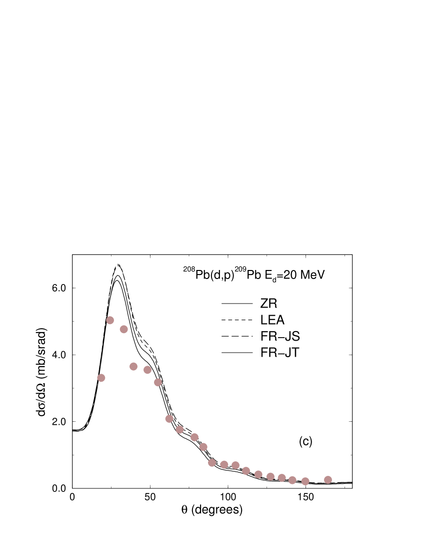
Figure 2: Angular distributions for (d,p) at energies slightly above the Coulomb barrier: (a) ⁶⁹Ga(d,p)⁷⁰Ga(g.s.) $E_{d}=12$ MeV (data from ga69 ), (b) ⁸⁶Kr(d,p)⁸⁷Kr(g.s.) $E_{d}=11$ MeV (data from kr86 ) and (c) ²⁰⁸Pb(d,p)²⁰⁹Pb(g.s.) $E_{d}=20$ MeV (data from pb208-20 ). Comparison of zero-range plus Johnson and Soper method (dotted), the LEA plus Johnson and Soper method (dashed), a finite range calculation of the transfer amplitude using the Johnson and Soper adiabatic potential (long-dashed) with the full finite range results (solid line).

Most of the available (d,p) data on stable systems was taken at energies above the Coulomb barrier for 10-20 MeV deuterons. In Fig. 2(a) we show results for ⁶⁹Ga(d,p)⁷⁰Ga at $E_{lab}=12$ MeV, in Fig. 2(b) ⁸⁶Kr(d,p)⁸⁷Kr at $E_{lab}=11$ MeV and in Fig. 2(c) ²⁰⁸Pb(d,p)²⁰⁹Pb at $E_{lab}=20$ MeV. The overall effect of finite range in all three cases is very small ($-1\%$ for the ⁶⁹Ga, $0.4\%$ for the ⁸⁶Kr and 6% in ²⁰⁸Pb), although it results from the cancellation of the two separate effects, the finite range in the deuteron potential, which reduces the cross section and the finite range effect in the evaluation of the T-matrix which increases the cross section. No simple addition rule for these two effects was found. Here, the local energy approximation begins to show larger deviations from the full finite range calculation.

Finally, we also consider reactions at higher energies (50-80 MeV deuteron energy). Only two data sets are available, namely for ¹²C and ⁴⁸Ca but we also include a study for ¹²⁴Sn and ²⁰⁸Pb to ensure that our results are not biased by lower mass systems. All cases studied at these energies reveal that finite range effects are large and reduce the cross section. In Fig. 3(a) we show the angular distributions for ¹²C(d,p)¹³C at $E_{lab}=56$ MeV, in Fig. 3(b) those for ⁴⁸Ca(d,p)⁴⁹Ca at $E_{lab}=56$ MeV and in Fig. 3(c) those for ¹²⁴Sn(d,p)¹²⁴Sn at $E_{lab}=70$ MeV. The overall effect of finite range at the peak of the distribution is $-36\%$ for ¹²C, $-24\%$ for ⁴⁸Ca and $-43.5$% for ¹²⁴Sn. It is the finite range in the adiabatic potential that is the dominant cause for these large changes although the finite-range effect in the evaluation of the T-matrix is still important and should not be neglected. In addition, for these higher energies, we find that the LEA method breaks down and for the heavier systems this approximation can in fact provide a correction in the opposite direction to the full finite range calculation.

Because it is the adiabatic scattering wavefunction that is mostly responsible for the large differences, we investigated the radial behavior of the scattering wavefunctions using either $U_{JT}$ or $U_{JS}$ for the partial waves which contribute the most to the transfer cross section. We specifically looked at the properties of the integrand of Eq.(16) in the zero-range approximation where it has a simpler form. We found that the percentage difference comes from subtle cancellations and cannot be well illustrated in the partial wave expansion. Intuitively one might argue that since the energies are larger, the dominant contribution to the transfer cross section comes from smaller impact parameters and thus sensitivity to the range of $V_{np}$ should be larger.

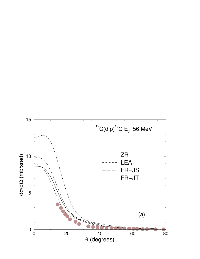
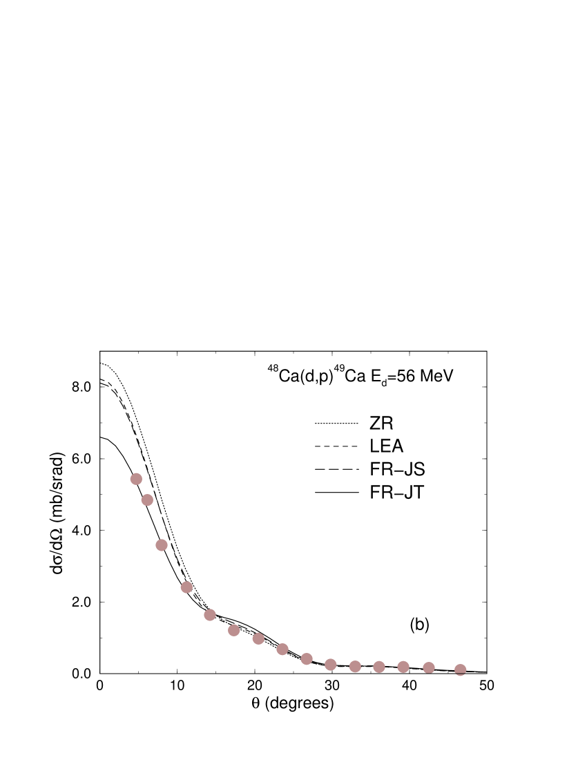
Figure 3: Angular distributions for (d,p) at high energies: (a) ¹²C(d,p)¹³C(g.s.) $E_{d}=56$ MeV (data from c12-56 ), (b) ⁴⁸Ca(d,p)⁴⁹Ca(g.s.) $E_{d}=56$ MeV (data from ca48-56 ) and (c) ¹²⁴Sn(d,p)¹²⁵Sn(g.s.) $E_{d}=70$ MeV. Comparison of zero-range plus Johnson and Soper method (dotted), the LEA plus Johnson and Soper method (dashed), a finite range calculation of the transfer amplitude using the Johnson and Soper adiabatic potential (long-dashed) with the full finite range results (solid line).

To ensure that our results are general, in particular that they will still be applicable to reactions in which the final bound state has a large spatial extension, we performed additional calculations for a fictitious ⁴⁸Ca(d,p)⁴⁹Ca setting the valence neutron angular momentum in the final bound state to $\ell=0$ state, and varying the binding energy $S_{n}=0.1-6$ MeV. The overall findings did not change: regardless of the loosely bound nature of the final nucleus, or the angular momentum in the final bound state, the effects of finite range in the transfer cross section are modest for low energies and become very important for the higher energies.

IV Discussion

The overall features obtained in this work can be best summarized in Fig.4 where the two separate effects of finite range are plotted as a function of beam energy for (d,p) reaction on four different targets: solid symbols provide the percentage effect of including finite range in the evaluation of the matrix element relative to a zero-range $T$-matrix calculation with a Johnson and Soper potential in both cases, and the open symbols correspond to the effect of including finite range effects in the distorting potential in the incident channel wave. The figure summarizes the results already given in Table 2. From this figure we can see that at low energy, finite range results differ by less than 10% from zero range matrix element with a Johnson and Soper adiabatic potential. However, as the incoming deuteron energy increases, finite range effects become very important and can dominate the result. The energy at which the transition occurs depends non linearly on the charge and the mass of the system. For practical purposes we find the transition to be around 20 MeV/u for lighter systems and 30 MeV/u for the heavy systems.

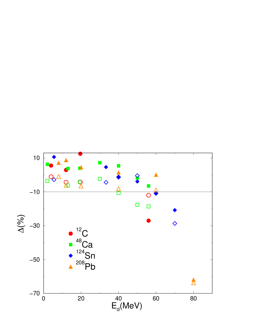
Figure 4: Systematic finite range effect as a function of beam energy: open symbols give the effect in the incident channel distorted wave, and the filled symbols are the effect in the evaluation of the matrix elements.

To facilitate the practical analysis of experiments, we searched for a global correction factor, a factor that would estimate the finite range effect as a function of target charge, mass and beam energy. Although for a given target one could always find a function $F(E_{d})$ representing the finite-range correction, no consistent dependence in mass and charge was found for the parameters of the various fits.

It is important to remember that the exact inclusion of deuteron finite range effects requires the solution of a couple channel equations Eq.(12) and here we truncated the Weinberg expansion to the first term to simplify the problem. The full equations were solved in laid for ⁶⁶Zn. It would be interesting to extend this study to better determine the range of validity of the truncation here used.

V Conclusion

We perform a systematic study of the effects of deuteron finite range in (d,p) reactions, within a formalism that includes the coherent effects of deuteron breakup through an adiabatic potential in the incident channel. We use the adiabatic formalism developed by Johnson and Soper soper in zero range and compare with the finite range generalization of Tandy and Johnson tandy . We analyze separately the effects of finite-range in the adiabatic distorting potential and finite range in the evaluation of the transfer matrix element. We also test the local energy approximation which is widely used as an estimate of finite range corrections to zero range transfer cross sections. We performed (d,p) calculations to determine angular distributions for a wide range of beam energies as well as a variety of targets, from A=12 to A=208.

For sub-Coulomb reactions, the percentage difference between the finite range and the zero range cross sections at the peak of the angular distribution relative to the zero range Johnson and Soper prediction is within 10% for all cases studied, and the local energy approximation provides an estimate within a few percent of the full finite range calculation. However, as the beam energy increases, finite range effects become more important. For intermediate energies ($E<20$ MeV/u for $A<50$ and $E<30$ MeV/u for heavier nuclei), including the finite range of the $n-p$ interaction in the adiabatic scattered wavefunction reduces the cross section while including finite range in the evaluation of the transfer amplitude increases the cross section. Both effects are significant, although strong cancellations may occur. At higher energies, both finite range effects have the same sign, reducing the transfer cross section. In this case we find the total effect of finite range to be very important. Our results also suggest that at these higher energies, the local energy approximation is no longer adequate.

This work was partially supported by the National Science Foundation grant PHY-0555893 and the Department of Energy under contract DE-FG52-08NA28552. RCJ is also partially supported by the United Kingdom Science and Technology Facilities Council under Grant No. ST/F012012.

References

- (1) H. Niewodniczanski, J. Nurzynski, A. Strzalkowski and G.R. Satchler, Phys. Rev. 146, 799 (1966).
- (2) W.W. Daehnick and Y.S. Park, Phys. Rev. 180, 1062 (1969).
- (3) D.E. Bainum, R.W. Finlay, J. Rapaport, J.D. Carlson and W.G. Love, Phys. Rev. C 16, 1377 (1977).
- (4) J.P. Schiffer et al., Phys. Rev. Lett 92, 162501 (2004).
- (5) M.B. Tsang, Jenny Lee, W.G. Lynch, Phys. Rev. Lett 95, 222501 (2005).
- (6) Jenny Lee et al., Phys. Rev. C 73, 044608 (2006).
- (7) Jenny Lee, M.B. Tsang and W.G. Lynch, Phys. Rev. C 75, 064320 (2007).
- (8) M.B. Tsang et al., Phys. Rev. Lett. 102, 062501 (2009).
- (9) Jenny Lee, M.B. Tsang, W.G. Lynch, M. Horoi, S.C. Su, Phys. Rev. C 79, 054611 (2009).
- (10) A. H. Wuosmaa et al., Phys. Rev. Lett. 94, 082502 (2005).
- (11) A. H. Wuosmaa et al., Phys. Rev. C72, 061301 (2005).
- (12) H.B. Jeppesen et al., Phys. Lett. B 642, 449 (2006).
- (13) J. S. Thomas et al., Phys. Rev. C76, 044302 (2007).
- (14) W N Catford et al., J. Phys. G 31, S1655 (2005).
- (15) A. Gade et al., Phys. Rev. C 77, 044306 (2008).
- (16) G.J. Kramer, H.P. Blok and L. Lapikas, Nucl. Phys. A 679, 267 (2001).
- (17) Jenny Lee et al., Phys. Rev. Lett. 104, 112701 (2010).
- (18) C. Barbieri, Phys. Rev. Lett. 103, 202502 (2009).
- (19) N. K. Timofeyuk, Phys. Rev. Lett. 103, 242501 (2009).
- (20) Ian Thompson and Filomena Nunes, Nuclear Reactions for Astrophysics, Cambridge University Press, Cambridge 2009.
- (21) N. Timofeyuk and R.C. Johnson, Phys. Rev. C 59, 1545 (1999).
- (22) E.O.Alt, P.Grassberger and W.Sandhas, Nucl.Phys. B 2, 167 (1967).
- (23) R.C. Johnson, Phys. Rev. C 80, 044616 (2009).
- (24) X. D. Liu, M. A. Famiano, W. G. Lynch, M. B. Tsang, and J. A. Tostevin, Phys. Rev. C69, 064313 (2004).
- (25) F. Delaunay, F. M. Nunes, W. G. Lynch, and M. B. Tsang, Phys. Rev. C72, 014610 (2005).
- (26) A. M. Mukhamedzhanov and F. M. Nunes, Phys. Rev. C72, 017602 (2005).
- (27) D. Y. Pang, F. M. Nunes, A. M. Mukhamedzhanov, Phys. Rev. C75, 024601 (2007).
- (28) R.C. Johnson and P.J.R. Soper, Phys. Rev. C1, 976 (1970).
- (29) P.J.A. Buttle and L.J.B. Goldfarb, Proc. Phys. Soc. 83, 701 (1964).
- (30) J.D. Harvey and R.C. Johnson, Phys. Rev. C3, 636 (1971).
- (31) R.C. Johnson, in ”Reaction Mechanisms for Rare Isotope Beams”, 2nd Argonne/MSU/JINA/INT RIA workshop. MSU, East Lansing, 9-12 March, 2005, (ed. by B.A. Brown) AIP Conf. Conf. Procs. 79, 128 (2005).
- (32) R.C. Johnson and P.C. Tandy, Nucl. Phys. A235, 56 (1974).
- (33) A. Laid, J. A. Tostevin, and R. C. Johnson, Phys. Rev. C 48, 1307 (1993).
- (34) V. Reid, Ann. Phys. (N.Y.) 50, 411 (1968).
- (35) R. L. Varner et al., Phys. Rep. 201, 57 (1991).
- (36) M. Igarashi et al., computer program TWOFNR, University of Surrey version, 2008.
- (37) G.L. Wales and R.C. Johnson, Nucl. Phys. A 274, 168 (1976).
- (38) M. Kamimura, M. Yahiro, Y. Iseri, H. Kameyama, Y. Sakuragi, and M. Kawai, Prog. Theor. Phys. Suppl. 89, 1 (1986).
- (39) I. J. Thompson, Comput. Phys. Rep. 7, 167 (1988).
- (40) G.M. Crawley, B.V.N. Rao, D.L. Powell, Nucl.Phys. A 112, 223(1968).
- (41) J. Rapaport, A. Sperduto and M. Salomaa, Nucl. Phys. A 197, 337 (1972).
- (42) J.L. Yntema, Phys. Rev. C 7, 140 (1973).
- (43) K. Haravu, C.L. Hollas, P.J. Riley, W.R. Coker, Phys. Rev.C 1, 938 (1970).
- (44) D.G. Kovar, N. Stein, C.K. Bockelman, Nucl. Phys. A 231, 266 (1974).
- (45) K. Hatanaka et al., Nucl. Phys.A 419, 530 (1984).
- (46) Y. Uozumi et al., Nucl. Phys. A 576, 123 (1994).