Absence of evidence is not evidence of absence: the color-density relation at fixed stellar mass persists to $z\sim 1$

Abstract

We use data drawn from the DEEP2 Galaxy Redshift Survey to investigate the relationship between local galaxy density, stellar mass, and rest-frame galaxy color. At $z\sim 0.9$, we find that the shape of the stellar mass function at the high-mass $(\log_{10}({\rm M}_{*}/h^{-2}\ {\rm M}_{\sun})>10.1)$ end depends on the local environment, with high-density regions favoring more massive systems. Accounting for this stellar mass-environment relation (i.e., working at fixed stellar mass), we find a significant color-density relation for galaxies with $10.6<\log_{10}({\rm M}_{*}/h^{-2}\ {\rm M}_{\sun})<11.1$ and $0.75<z<0.95$. This result is shown to be robust to variations in the sample selection and to extend to even lower masses (down to $\log_{10}({\rm M}_{*}/h^{-2}\ {\rm M}_{\sun})\sim 10.4$). We conclude by discussing our results in comparison to recent works in the literature, which report no significant correlation between galaxy properties and environment at fixed stellar mass for the same redshift and stellar mass domain. The non-detection of environmental dependence found in other data sets is largely attributable to their smaller samples size and lower sampling density, as well as systematic effects such as inaccurate redshifts and biased analysis techniques. Ultimately, our results based on DEEP2 data illustrate that the evolutionary state of a galaxy at $z\sim 1$ is not exclusively determined by the stellar mass of the galaxy. Instead, we show that local environment appears to play a distinct role in the transformation of galaxy properties at $z>1$.

1. Introduction

With the emergence of large spectroscopic surveys at intermediate redshift, such as the DEEP2 Galaxy Redshift Survey (Davis et al., 2003; Newman et al., 2010), the VIMOS VLT Deep Survey (VVDS, Le Fèvre et al., 2005), and zCOSMOS (Lilly et al., 2007), robust systematic studies of galaxy clustering are now able to be extended out to $z\sim 1$ (e.g., Coil et al., 2004b, 2006; Meneux et al., 2008, 2009). In particular, these unprecedented data sets have enabled the local density of galaxies (i.e., on scales of $\sim\!1$–$2$ $h^{-1}$ Mpc) to be statistically measured over a broad and continuous range of environments extending from voids to rich groups and poor clusters at $z\sim 1$ (e.g., Cooper et al., 2005, 2006; Cucciati et al., 2006; Kovac et al., 2010). Moreover, individual galaxy groups at $z\sim 1$ are now able to be reliably identified in redshift space, enabling the “field” population to be studied in relation to the “group” or “cluster” population (e.g., Gerke et al., 2005; Knobel et al., 2009; Cucciati et al., 2009).

Capitalizing on the ability to characterize environment over half of the age of the Universe, many studies have addressed the role of environment in galaxy evolution at $z<1$ by studying the relationship between environment and galaxy properties such as rest-frame color and morphology (e.g., Gerke et al., 2007; Elbaz et al., 2007; Capak et al., 2007; Cooper et al., 2008). For example, using data drawn from the DEEP2 survey, Cooper et al. (2006) showed that all features of the global correlation between galaxy color and environment measured locally are already in place at $z\sim 1$ (see also Coil et al., 2008). This work emphasized that physical processes specific to clusters (such as ram-pressure stripping and harassment) are not required to explain the color-density relation at $z\sim 1$, given the lack of such extreme environments in the DEEP2 sample.

However, as highlighted by several recent analyses, nearly all of the early studies addressing the relationships between environment and galaxy properties at intermediate redshift primarily utilized luminosity-selected samples and not stellar mass-selected samples. A number of recent papers have concluded that while there is evidence for a color-density relation at fixed luminosity at $z\sim 1$, they find no color-density relation at fixed mass. For example, Scodeggio et al. (2009) employ data from VVDS to examine the relationship between rest-frame $B-I$ color and environment as a function of redshift within fixed bins of stellar mass. They find no evidence for a color-density relation at fixed mass over the entire redshift $(0.2<z<1.4)$ and stellar mass $(9<\log_{10}({\rm M}_{*})<11)$ ranges probed by their data. Using zCOSMOS to characterize the local environment, Tasca et al. (2009) also find that at $0.5<z<1$ there is no variation in galaxy morphology (i.e., early- versus late-type) as a function of local galaxy density at stellar masses of $\log_{10}({\rm M}_{*}/h^{-2}\ {\rm M}_{\sun})>10.5$. From these results, both of the aforementioned studies conclude that the properties (i.e., color and morphology) of massive galaxies are independent of environment at $z\sim 1$.

Given the substantial noise in all current measures of environment (both statistical measures of the local galaxy density and group/field catalogs), intrinsic correlations between galaxy properties and environment can easily be smeared out, such that no significant trends with environment are detectable in the data. That is, it is far easier to smear out a correlation with environment than it is to erroneously detect one as, generally, measures of local density are dependent on redshift measurements of neighboring galaxies, while a given galaxy’s properties are measured from its own imaging and spectroscopic data. It is difficult to imagine a systematic effect that would yield a false correlation between independently determined quantities.

Conclusions based on the lack of an apparent environment dependence must therefore be drawn with caution. In this paper, we use data from the DEEP2 survey to investigate the significance or robustness of the recent, aforementioned conclusions inferred from studies of galaxy environments at intermediate redshift. In Section 2, we describe our data set, with results and discussion presented in Sections 3 and 4, respectively. Throughout, we employ a $\Lambda$CMD cosmology with $w=-1$, $\Omega_{m}=0.3$, $\Omega_{\Lambda}=0.7$, and a Hubble parameter of $H_{0}=100\ h$ km s^-1 Mpc^-1. All magnitudes are on the AB system.

2. Data

Among the current generation of deep spectroscopic redshift surveys at $z\sim 1$, the DEEP2 Galaxy Redshift Survey provides the largest sample of accurate spectroscopic redshifts, the highest-precision velocity information, and the highest sampling density. Altogether, these attributes make the DEEP2 survey the best existing spectroscopic data set with which to characterize local environment. In this paper, we utilize a sample of $23,037$ galaxies with accurate redshifts (quality $Q=3$ or 4 as defined by Newman et al., 2010) in the range $0.75<z<1.25$ and drawn from all four of the DEEP2 survey fields.

For each galaxy in the DEEP2 sample, rest-frame $U-B$ colors and absolute $B$-band magnitudes, $M_{B}$, are calculated from CFHT $BRI$ photometry (Coil et al., 2004a) using the $K$-correction procedure described in Willmer et al. (2006). For a portion of the DEEP2 catalog, stellar masses may be calculated by fitting spectral energy distributions (SEDs) to WIRC/Palomar $J$- and $K_{s}$-band photometry in conjunction with the DEEP2 $BRI$ data, according to the prescriptions described by Bundy et al. (2005, 2006). However, the near-infrared photometry, collected as part of the Palomar Observatory Wide-field Infrared (POWIR, Conselice et al., 2008) survey, does not cover the entire DEEP2 survey area, and often faint blue galaxies at the high-$z$ end of the DEEP2 redshift range are not detected in $K_{s}$. Because of these two effects, the stellar masses of Bundy et al. (2006) have been used to calibrate stellar mass estimates for the full DEEP2 sample that are based on rest-frame $M_{B}$ and $B-V$ values derived from the DEEP2 data in conjunction with the expressions of Bell et al. (2003). We empirically correct these stellar mass estimates to the Bundy et al. (2006) measurements by accounting for a mild color and redshift dependence (Lin et al., 2007); where they overlap, the two stellar masses have an rms difference of approximately $0.3$ dex after this calibration.

To characterize the local environment, we compute the projected third-nearest-neighbor surface density $(\Sigma_{3})$ about each galaxy in the DEEP2 sample, where the surface density depends on the projected distance to the third-nearest neighbor, $D_{p,3}$, as $\Sigma_{3}=3/(\pi D_{p,3}^{2})$. In computing $\Sigma_{3}$, a velocity window of $\pm 1000$ km s^-1 is utilized to exclude foreground and background galaxies along the line of sight. Varying the width of this velocity window (e.g., using $\pm 1500$ km s^-1) or tracing environment according to the projected distance to the fifth-nearest neighbor has no significant effect on our results. In the tests of Cooper et al. (2005), this projected $n^{\rm th}$-nearest-neighbor environment estimator proved to be the most robust indicator of local galaxy density for the DEEP2 survey.

To correct for the redshift dependence of the DEEP2 sampling rate, each surface density value is divided by the median $\Sigma_{3}$ of galaxies at that redshift within a window of $\Delta z=0.04$; correcting the measured surface densities in this manner converts the $\Sigma_{3}$ values into measures of overdensity relative to the median density (given by the notation $1+\delta_{3}$ here) and effectively accounts for the redshift variations in the selection rate (Cooper et al., 2005). Finally, to minimize the effects of edges and holes in the survey geometry, we exclude all galaxies within $1$ $h^{-1}$ comoving Mpc of a survey boundary, reducing our sample to $17,767$ galaxies in the redshift range $0.75<z<1.25$.

Figure 1.— the rest-frame $U-B$ versus $M_{B}$ color-magnitude distribution for DEEP2 galaxies in the spectroscopic sample within the redshift range $0.75<z<1.25$. The three solid black vertical lines show the completeness limit of the survey at $z=0.9$, $1.05$, and $1.25$, while the solid and dashed red lines show lines of constant stellar mass corresponding to $\log_{10}({\rm M}_{*}/h^{-2}\ {\rm M}_{\sun})=10.6$ and $10.8$, respectively. The dashed blue/red horizontal line shows the division between the red sequence and the blue cloud as given by Equation 19 from Willmer et al. (2006).

To investigate the relationship between galaxy properties and environment within the high-mass segment of the galaxy population, we define a subsample of galaxies with stellar mass in the range $10.6<\log_{10}({\rm M}_{*}/h^{-2}\ {\rm M}_{\sun})<11.1$ and a redshift of $0.75<z<1.05$. The median redshift for this subsample of $1586$ galaxies is $0.89$ and the median stellar mass is $\log_{10}({\rm M}_{*}/h^{-2}\ {\rm M}_{\sun})\sim 10.8$. We restrict the subsample in redshift to a range over which the DEEP2 redshift selection function is relatively flat. However, over this redshift range the sample is incomplete at the adopted mass limit. For example, at $z=0.9$ the $R_{\rm AB}=24.1$ magnitude limit of DEEP2 includes all galaxies with stellar mass $>\!10^{10.8}\ {\rm M}_{*}/h^{-2}\ {\rm M}_{\sun}$ independent of color, but preferentially misses red galaxies at lower masses (cf. Figure 1).

Figure 1 shows the distribution of galaxies in color-magnitude space for the entire DEEP2 sample at $0.75<z<1.25$, with lines of constant stellar mass overlaid. As shown in many previous studies (e.g., Bell & de Jong, 2001; Hogg et al., 2003; Cooper et al., 2008), selecting by stellar mass as opposed to optical luminosity selects a different portion of the galaxy population due to the dependence of stellar mass-to-light ratio on rest-frame color. A $B$-band luminosity-selected sample is biased towards lower stellar masses for blue galaxies and higher stellar masses for red galaxies.

Now, both locally and at $z\sim 1$, the local environment of galaxies on the red sequence has been shown to depend on luminosity such that more luminous systems favor higher-density regions on average (Blanton et al., 2005; Cooper et al., 2006). Thus, relative to a random population of blue galaxies, red galaxies of equivalent stellar mass will be (less luminous and) in lower-density environments than red galaxies selected to have the same luminosity. That is, taking into account the known correlation between local environment and galaxy luminosity, for a galaxy sample selected to have fixed stellar mass (versus fixed luminosity) one expects to find a weaker color-density relation. However, it remains unclear whether or not the correlation between galaxy environment and rest-frame color found at fixed luminosity at $z\sim 1$ (Cooper et al., 2006) is entirely a projection of the correlation between environment and luminosity in concert with the dependence of stellar mass-to-light ratio on color such that at fixed stellar mass there is no color-density relation. As discussed in §1, several recent analyses have arrived at this conclusion.

3. Analysis

As highlighted in §1, the goal of this work is to study the relationship between galaxy color and local environment at fixed stellar mass. Recent analyses using a variety of data sets have approached this task using galaxy samples in stellar-mass-selected bins across a range of environments. Here, we first investigate whether this methodology is appropriate. Finding it is not — that is, finding that the stellar mass function is different in different environments — we then apply improved techniques which account for the correlation between stellar mass and environment in an examination of the color-density relation at $z\sim 1$. In contrast to recent results in the literature, we find that there is a significant color-density relation at fixed stellar mass. The most likely reason for this discrepancy is that both larger measurement errors and systematics in other data sets smear out the underlying environment dependence. Finally, we emphasize that absence of evidence is not evidence of absence; that is, not finding a correlation between color and environment at fixed stellar mass does not directly indicate an intrinsic lack of correlation. By making such an assumption, the conclusions of several recent analyses have been rendered difficult to interpret.

3.1. The Relationship between Stellar Mass and Environment

In order to study the relationship between galaxy properties and environment at fixed stellar mass, the galaxy sample under study is often restricted to a narrow range in stellar mass such that correlations between stellar mass and environment are negligible. However, at intermediate redshift, sample sizes are generally limited in number such that using a particularly narrow stellar mass range (e.g., $\sim\!0.1$–$0.2$ dex in width) significantly reduces the statistical power of the sample. For this reason, broader stellar mass bins (e.g., $\sim\!0.5$ dex) are commonly employed (e.g., Scodeggio et al., 2009; Iovino et al., 2009; Patel et al., 2009; Kovac et al., 2009; Maltby et al., 2010). Now, if the shape of the stellar mass function depends on environment, then the typical stellar mass within a broad mass bin may differ significantly from one density regime to another. Such an effect would clearly impact the ability to study the color-density relation at fixed stellar mass.

To investigate the level to which we are sensitive to a stellar mass-environment relation within our adopted stellar mass bin, we select those galaxies within the top $10\%$ of the overdensity distribution for all galaxies at $10.6<\log_{10}({\rm M}_{*}/h^{-2}\ {\rm M}_{\sun})<11.1$ and $0.75<z<1.05$ — a subsample of $159$ galaxies. From the corresponding bottom $50\%$ of the overdensity distribution, we draw $1000$ random galaxy subsamples (each consisting of $159$ galaxies), where each subsample is selected to match the redshift distribution of the galaxies in the high-density subsample.

By matching in redshift, we remove the projection of any possible residual correlation between our environment measurements and redshift (in concert with the known redshift dependence of the survey’s stellar-mass limit) onto the observed stellar mass-environment relation. This effect appears to be impacting the analysis of Iovino et al. (2009). As shown in Figure 12 of that work, the typical redshift of “isolated” galaxies (i.e., galaxies in low-density environments) is systematically skewed towards higher $z$ relative to the sample of “group” members (i.e., galaxies in high-density environments). This effect is likely due to the decreasing sampling density of a magnitude-limited redshift survey at higher $z$, which introduces a bias against identifying groups at higher redshift. Note that our adopted stellar mass bins are well-matched to those of Iovino et al. (2009), taking into account differences in the adopted value of the Hubble parameter.

To test whether our high-density subsample and the random low-density subsamples are drawn from the same underlying stellar mass distribution, we apply the one-sided Wilcoxon-Mann-Whitney (WMW) $U$ test (Mann & Whitney, 1947), a non-parametric test that is highly robust to non-Gaussianity because it relies on ranks rather than observed values. The result of the WMW $U$ test is the probability ($P_{U}$) that a value of the $U$ statistic equal to the observed value or more extreme would result if the “null” hypothesis (that both samples are drawn from identical distributions) holds. The WMW $U$ test is particularly useful for small data sets (e.g., compared to other related tests such as the chi-square two-sample test, Wall & Jenkins 2003), as we have when selecting galaxies from a narrow stellar mass range and in extreme environments, due to its insensitivity to outlying data points, its avoidance of binning, and its high efficiency. Note that since this test is one-sided, possible $P_{U}$ values range from $0$ to $0.5$; for a $P_{U}$ value below $0.025$ (corresponding closely to $2\sigma$ for a Gaussian), we can reject the null hypothesis (that the two samples have the same distribution) at greater than $95\%$ significance.

In Figure 2, we plot the cumulative distribution of stellar masses for the $159$ sources in the high-density subsample along side that for the 1000 random subsamples (each consisting of $159$ galaxies) matched in redshift but residing in low-density environments. Performing a one-sided WMW $U$ test on the stellar mass measurements for the low- and high-density populations, we find that the stellar mass distribution for the galaxies in high-density environments is skewed to slightly higher stellar mass, with a probability of $P_{U}\sim 0.09$. Meanwhile, the cumulative redshift distributions for the low- and high-density subsamples, shown in the inset of Figure 2, are well-matched with the WMW $U$ test yielding a $P_{U}>0.48$, thus confirming that the redshift distributions for the two samples are indistinguishable and therefore not significantly contributing to the difference in the stellar mass distributions.

The results of the WMW $U$ test are supported by a comparison of the mean stellar masses for the low- and high-density subsamples, which are distinct at a $\gtrsim\!1.5\sigma$ level, thereby supporting the conclusion that there is a non-negligible stellar mass-environment relation within the given mass bin. In addition to directly comparing the arithmetic means of the stellar mass distributions, we also utilize the Hodges-Lehmann (H-L) estimator of the mean, which is given by the median value of the mean stellar mass computed over all pairs of galaxies in the sample (Hodges & Lehmann, 1963). Like taking the median of a distribution, the H-L estimator of the mean is robust to outliers, but, unlike the median, yields results with scatter (in the Gaussian case) comparable to the arithmetic mean. Thus, by using the H-L estimator of the mean, we gain robustness as in the case of the median, but unlike the median, our measurement errors are increased by only a few percent. In Figure 3, we show the distribution of differences between the Hodges-Lehmann estimator of the mean stellar mass for the high-density subsample relative to that for the $1000$ low-density subsamples, where the median difference in stellar mass is $\Delta\log_{10}({\rm M}_{*}/h^{-2}\ {\rm M}_{\sun})\sim 0.019$ as illustrated by the dotted vertical line. Within the stellar mass range of $10.6<\log_{10}({\rm M}_{*}/h^{-2}\ {\rm M}_{\sun})<11.1$, we find (by all of these methods) $\sim\!1.5\sigma$ evidence for a weak stellar mass-environment relation at $z\sim 0.9$ such that more massive galaxies favor higher-density regions.

This weak correlation between stellar mass and environment is robust to variations in the stellar mass and redshift ranges used to select the galaxy population. For example, pushing to slightly lower stellar masses ($10.2<\log_{10}({\rm M}_{*}/h^{-2}\ {\rm M}_{\sun})<10.7$), while still limiting the sample to a range of only $0.5$ dex, we again find evidence for a weak correlation between between stellar mass and environment (see Table 1). Expanding the range of stellar masses probed to $10.1<\log_{10}({\rm M}_{*}/h^{-2}\ {\rm M}_{\sun})<11.1$, the stellar mass-density relation is increasingly evident, such that we find a highly-significant correlation between stellar mass and environment at $z\sim 0.9$, with $P_{U}<0.01$. This result is in general agreement with existing studies of the projected galaxy correlation function as a function of stellar mass at $z\sim 1$ (e.g., Meneux et al., 2008; Foucaud et al., 2010), which find weak evidence that more massive galaxies are more strongly clustered on small scales. Likewise, measurements of the stellar mass function at slightly lower redshift $(z\sim 0.5)$ also suggest a variation in the shape of the mass function with local environment (Bolzonella et al., 2009; Kovac et al., 2009; Peng et al., 2010).

Thus, when looking to quantify environmental dependencies at fixed stellar mass, the use of broad stellar mass bins (e.g., those used by Scodeggio et al. 2009, Iovino et al. 2009, Tasca et al. 2009, Kovac et al. 2009, and Grützbauch et al. 2010) or simple mass-limited sample selections (e.g., van der Wel et al., 2007; Pannella et al., 2009; Rettura et al., 2010) is inappropriate as both approaches implicitly assume that there is no variation in the stellar mass function with environment. In the following subsection, we develop improved techniques that account for the apparent environmental dependence of the shape of the stellar mass function, thereby enabling an unbiased analysis of the color-density relation at fixed stellar mass.

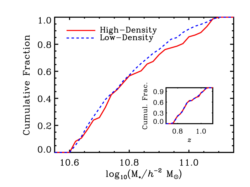
Figure 2.— the cumulative stellar mass and redshift (see inset) distributions for the $159$ DEEP2 galaxies comprising the top $10\%$ of the environment distribution within the stellar mass and redshift ranges of $10.6<\log_{10}({\rm M}_{*}/h^{-2}\ {\rm M}_{\sun})<11.1$ and $0.75<z<1.05$ in comparison to the corresponding cumulative distributions for the $1000$ random galaxy subsamples drawn from the lowest $50\%$ of the same environment distribution. As discussed in the text, the low-density subsamples, which are each composed of $159$ galaxies, are selected to have the same redshift distribution as the high-density population. However, the stellar mass distribution is found to be biased in the different environment regimes.

Figure 3.— the distribution of differences between the Hodges-Lehmann (H-L) estimator of the mean stellar mass (left) and mean redshift (right) for the high-density subsample relative to the corresponding H-L estimator of the mean for each of the $1000$ low-density subsamples. The median differences in stellar mass and redshift are denoted by the dotted vertical lines, while the dashed vertical lines and corresponding error bars show the difference in the arithmetic means (and uncertainty in that difference) for the low-density and high-density populations. We find a small offset in stellar mass of $\Delta\log_{10}({\rm M}_{*}/h^{-2}\ {\rm M}_{\sun})\sim 0.019$, while the difference in mean redshift of the two samples is consistent with zero (by construction). Within the broad stellar mass range of $10.6<\log_{10}({\rm M}_{*}/h^{-2}\ {\rm M}_{\sun})<11.1$, we detect a weak stellar mass-environment relation at $z\sim 0.9$ such that more massive galaxies favor higher-density regions.

3.2. The Color-Density Relation at Fixed Stellar Mass

The ultimate goal of this work is not to study the correlation between stellar mass and environment, but rather to investigate the relationship between galaxy color and environment at fixed stellar mass. But as shown in the above analysis, we must be careful to account for the weak correlation between stellar mass and overdensity even with stellar mass bins as narrow as $0.5$ dex. Thus, we now select those galaxies within the top $10\%$ of the overdensity distribution for all galaxies at $10.6<\log_{10}({\rm M}_{*}/h^{-2}\ {\rm M}_{\sun})<11.1$ and $0.75<z<1.05$ (the same high-density subsample of $159$ galaxies), and from the corresponding bottom $50\%$ of the overdensity distribution we randomly draw 1000 subsamples (each composed of $159$ galaxies) so as to match the joint redshift and stellar mass distributions of the galaxies in the high-density subsample. Members of the low-density subsample are drawn randomly from within a two-dimensional window with dimensions of $\Delta z^{2}<4\cdot 10^{-4}$ and $\Delta\log_{10}({\rm M}_{*})^{2}<5\cdot 10^{-5}$ of a randomly-selected object in the high-density subsample. Varying the size of this window by factors of a few in each dimension has no significant effect on our results. Given the random nature of the matching, some objects are repeated in the low-density subsamples. However, for each subsample of $159$ galaxies, $\sim\!90\%$ of the galaxies are unique; requiring all members of a subsample to be unique would skew the statistics (Efron, 1981). By matching our high- and low-density subsamples in stellar mass as well as redshift, we are able to effectively study the correlation between galaxy properties such as color and environment at fixed stellar mass.

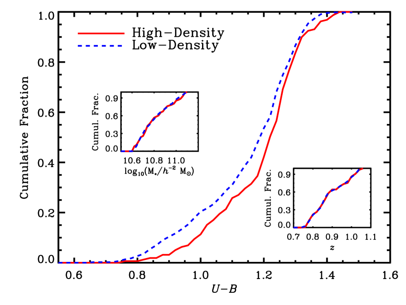
Figure 4.— the cumulative rest-frame $U-B$ color, stellar mass, and redshift distributions for the $159$ DEEP2 galaxies with the highest measured overdensities (the top $10\%$ of the environment distribution) within the stellar mass and redshift ranges of $10.6<\log_{10}({\rm M}_{*}/h^{-2}\ {\rm M}_{\sun})<11.1$ and $0.75<z<1.05$ in comparison to the corresponding cumulative distributions for the $1000$ random galaxy subsamples drawn from the lowest $50\%$ of the same environment distribution. As discussed in the text, the low-density subsamples, which are each composed of $159$ galaxies, are selected to have the same stellar mass and redshift distributions as the high-density population (see inset plots). For galaxies with stellar masses of $10.6<\log_{10}({\rm M}_{*}/h^{-2}\ {\rm M}_{\sun})<11.1$ at $z\sim 0.9$, we find a significant color-density relation at fixed stellar mass such that red galaxies preferentially reside in overdense regions relative to their bluer counterparts.

As shown in Figures 4 and 5, we find a significant relationship at $z\sim 0.9$ between rest-frame $U-B$ color and local galaxy overdensity at fixed stellar mass for galaxies with $10.6<\log_{10}({\rm M}_{*}/h^{-2}\ {\rm M}_{\sun})<11.1$. The cumulative color distributions for the two subsamples drawn from separate environment regimes are significantly distinct, with the galaxies in high-density environments skewed towards redder rest-frame colors. The WMW $U$ test confirms what is apparent in Figure 4, yielding $P_{U}<0.002$ when comparing the color distributions of the high- and low-density subsamples: these color distributions are distinct at $>\!3\sigma$ confidence. By construction, the corresponding stellar mass and redshift distributions are indistinguishable (see inset plots in Fig. 4), with $P_{U}\sim 0.47$ and $P_{U}\sim 0.49$, respectively.

In Figure 5, we show the distribution of differences between the Hodges-Lehmann estimator of the mean $U-B$ color, stellar mass, and redshift for the high-density subsample relative to the corresponding estimator of the mean for the $1000$ low-density subsamples. The median differences in stellar mass and redshift are consistent with zero, $\Delta z\sim-1\cdot 10^{-4}\pm 0.009$ and $\Delta\log_{10}({\rm M}_{*}/h^{-2}\ {\rm M}_{\sun})\sim 0.003\pm 0.012$, while the median offset in rest-frame color is $\Delta(U-B)\sim 0.033\pm 0.013$ such that galaxies in high-density environs are typically redder in color at fixed stellar mass and redshift. Similarly, the arithmetic means of the two color distributions are accordingly found to be distinct at $\gtrsim\!3.5\sigma$ (see Table 2). Altogether, the DEEP2 data show a robust color-density relation at fixed stellar mass at $z\sim 0.9$ for galaxies in the stellar mass regime of $10.6<\log_{10}({\rm M}_{*}/h^{-2}\ {\rm M}_{\sun})<11.1$.

Figure 5.— the distribution of differences between the Hodges-Lehmann (H-L) estimator of the mean $U-B$ color, redshift, and stellar mass for the high-density subsample relative to the corresponding H-L estimator of the mean for each of the $1000$ low-density subsamples. The median differences in $U-B$, $z$, and stellar mass are denoted by the dotted vertical lines, while the dashed vertical lines and corresponding error bars show the difference in the arithmetic means (and uncertainty in that difference) for the low-density and high-density populations (taken as a whole). Recall that the redshift and stellar mass distributions of the low- and high-density samples match by construction. We find a significant offset in rest-frame color of $\Delta(U-B)\sim 0.04$, while the difference in mean redshift and stellar mass for the two samples is consistent with zero.

To test the robustness of our results to the particularities of the sample selection, we repeat the analysis described above for several samples spanning varying redshift and stellar mass regimes. For example, broadening the redshift range over which we select galaxies to $0.75<z<1.25$, thereby increasing the size of the sample, we again find a statistically significant relationship between rest-frame color and environment within our adopted stellar mass bin of $10.6<\log_{10}({\rm M}_{*}/h^{-2}\ {\rm M}_{\sun})<11.1$. For the $211$ galaxies in the high-density regime (again the highest $10\%$ of the overdensity distribution) at $0.75<z<1.25$, the cumulative distribution of $U-B$ color is skewed towards redder colors relative to the comparison set of galaxies in low–density environments, yielding $P_{U}<0.01$ and with the means of the two color distributions distinct at a $\sim\!3\sigma$ level. In Table 2, we list the results from similar analyses of several other galaxy samples. When varying the redshift and/or stellar mass regimes probed, we continue to find a significant color-density relation at fixed stellar mass at $z\sim 1$. This result is found to hold even at slightly lower masses; restricting to only those galaxies with $10.2<\log_{10}({\rm M}_{*}/h^{-2}\ {\rm M}_{\sun})<10.7$ (a sample with a median stellar mass of $\log_{10}({\rm M}_{*}/h^{-2}\ {\rm M}_{\sun})\sim 10.4$), we again find that redder galaxies tend to favor overdense regions at fixed stellar mass and redshift.

Table 1 Summary of Results for Stellar Mass-Density Relation at Fixed Redshift

Sample	$N_{\rm high-density}$	$P_{U}(z)$	$P_{U}(\log_{10}({\rm M}_{*}))$	$\Delta z$	$\Delta\log_{10}({\rm M}_{*})$
$0.75<z<1.05$	$159$	$0.49$	$0.09$	$0.000\pm 0.007$	$0.019\pm 0.012$
$10.6<\log_{10}({\rm M}_{*})<11.1$
$0.75<z<1.05$	$456$	$0.48$	$<\!0.01$	$0.000\pm 0.004$	$0.051\pm 0.012$
$10.1<\log_{10}({\rm M}_{*})<11.1$
$0.75<z<1.25$	$211$	$0.49$	$0.13$	$0.000\pm 0.005$	$0.012\pm 0.010$
$10.6<\log_{10}({\rm M}_{*})<11.1$
$0.75<z<1.05$	$273$	$0.49$	$0.08$	$0.000\pm 0.006$	$0.012\pm 0.008$
$10.2<\log_{10}({\rm M}_{*})<10.7$

Note. — For a variety of galaxy samples, we list the results of the WMW $U$ test ($P_{U}$) and the difference in the arithmetic means computed from a comparison of the redshift and stellar mass distributions of the respective low- and high-density samples. The $P$-value, $P_{U}$, indicates the probability that differences in the distribution of the stated quantity as large as those observed (or larger) would occur by chance if the two samples shared identical distributions. The number of galaxies in the high-density sample (picked to be the top 10% of the environment distribution) is given by $N_{\rm high-density}$. Note that the difference in the mean for the galaxy property $x$ is given by $<{x}_{\rm high-density}>-<{x}_{\rm low-density}>$ and that stellar masses are in units of $h^{-2}\ {\rm M}_{\sun}$.

Table 2 Summary of Results for Color-Density Relation at Fixed Stellar Mass and Redshift

Sample	$N_{\rm high-density}$	$P_{U}(z)$	$P_{U}(\log_{10}({\rm M}_{*}))$	$P_{U}(U-B)$	$\Delta z$	$\Delta\log_{10}({\rm M}_{*})$	$\Delta(U-B)$
$0.75<z<1.05$	$159$	$0.49$	$0.47$	$<\!0.01$	$0.000\pm 0.007$	$0.002\pm 0.012$	$0.040\pm 0.011$
$10.6<\log_{10}({\rm M}_{*})<11.1$
$0.75<z<0.95$	$101$	$0.48$	$0.47$	$0.01$	$0.000\pm 0.005$	$0.002\pm 0.015$	$0.043\pm 0.014$
$10.6<\log_{10}({\rm M}_{*})<11.1$
$0.75<z<1.25$	$211$	$0.47$	$0.46$	$<\!0.01$	$0.000\pm 0.008$	$0.002\pm 0.010$	$0.032\pm 0.010$
$10.6<\log_{10}({\rm M}_{*})<11.1$
$0.75<z<1.05$	$456$	$0.48$	$0.46$	$<\!0.01$	$0.000\pm 0.004$	$0.003\pm 0.012$	$0.029\pm 0.009$
$10.1<\log_{10}({\rm M}_{*})<11.1$
$0.85<z<1.15$	$404$	$0.47$	$0.49$	$0.02$	$0.000\pm 0.004$	$0.002\pm 0.013$	$0.019\pm 0.010$
$10.1<\log_{10}({\rm M}_{*})<11.1$
$0.75<z<1.05$	$273$	$0.49$	$0.47$	$<\!0.01$	$0.000\pm 0.006$	$0.000\pm 0.008$	$0.032\pm 0.011$
$10.2<\log_{10}({\rm M}_{*})<10.7$

Note. — For a variety of galaxy samples, we list the results of the WMW $U$ test ($P_{U}$) and the difference in the arithmetic means computed from a comparison of the redshift, stellar mass, and color distributions of the respective low- and high-density samples. The $P$-value, $P_{U}$, indicates the probability that differences in the distribution of the stated quantity as large as those observed (or larger) would occur by chance if the two samples shared identical distributions. The number of galaxies in the high-density sample (picked to be the top 10% of the environment distribution) is given by $N_{\rm high-density}$. Note that the difference in the mean for the galaxy property $x$ is given by $<{x}_{\rm high-density}>-<{x}_{\rm low-density}>$ and that stellar masses are in units of $h^{-2}\ {\rm M}_{\sun}$. Finally, note that the galaxy samples listed here are distinct from those detailed in Table 1. These samples are matched in redshift as well as stellar mass.

4. Discussion

As shown in Figure 4, we find that there exists a correlation between rest-frame $U-B$ color and local galaxy overdensity within the high-mass ($\log_{10}({\rm M}_{*}/h^{-2}\ {\rm M}_{\sun})\sim 10.8$) segment of the galaxy population at $z\sim 0.9$ such that red galaxies favor higher-density environments at fixed stellar mass. As noted in Section 1, several recent studies utilizing data from VVDS and zCOSMOS have concluded that no such correlation exists within this stellar mass and redshift regime (e.g., Scodeggio et al., 2009; Iovino et al., 2009). Here, we discuss the likely reasons for the discrepancy between these conclusions and our results.

It is highly unlikely that the highly significant color-density relation at fixed stellar mass within the DEEP2 data is spurious. Rest-frame galaxy colors and stellar masses, which depend on the adopted stellar population models, photometry, and only coarsely on redshift, are entirely independent of the environment measures, which depend upon angular position and high-precision redshift information (both for the galaxy in question and neighboring galaxies). There is no reasonable mechanisms that would produce a false correlation between these independent quantities. For instance, one might suggest that contamination of photometry is an issue in dense regions; however, even in the most overdense environments (e.g., the top $5\%$ of the environment distribution), the typical distance to the $3^{\rm rd}$-nearest neighbor corresponds to $\sim\!35^{\prime\prime}$ on the sky, which is much larger than the aperture sizes used in photometry. Instead, as highlighted in Section 1, it is far more likely that the color-density relation apparent in DEEP2 has been smeared out in studies using other data sets due to the smaller sample sizes employed and the significantly larger errors in the environment measures derived from those data sets.

Many of the limitations regarding the VVDS data set, as they relate to detecting correlations between galaxy properties and environment at $z\sim 1$, are discussed at length by Cooper et al. (2007) in a comparison to the work by Cucciati et al. (2006). Using DEEP2 data, Cooper et al. (2007) find a significant correlation between rest-frame galaxy color and environment at $M_{B}<-20.5-5\cdot\log_{10}(h)$ and $0.9<z<1.2$, where none is evident in the analysis of VVDS data presented by Cucciati et al. (2006). While both of these studies employed luminosity-selected galaxy samples, the lessons learned from the comparison are no less applicable to analyses of samples selected according to stellar mass. Here, we review the arguments presented by Cooper et al. (2007) as they relate to the more recent analyses using VVDS, zCOSMOS, and other data sets.

At $z\gtrsim 0.75$, the sample size of both VVDS and zCOSMOS are significantly smaller than that collected by DEEP2. At these redshifts, DEEP2 has more than $26,891$ secure ($95\%$ or greater confidence) redshifts, while the VVDS and zCOSMOS data sets include only $1,581$ and $967$ high-quality (i.e., $\rm{flag}\!=\!3,4$) redshifts, respectively.

In addition to their smaller statistical power relative to DEEP2, both VVDS and zCOSMOS have a significantly lower number density of tracer objects (cf. Newman et al., 2010), which directly influences the level to which the resulting data sets can trace local galaxy density. Crudely, errors on overdensity measurements on some length scale should be dominated by Poisson statistics and hence should be proportional to the square root of the number density of tracers. To test the impact of a reduction in the sampling density, we dilute the DEEP2 data set by a factor of $3$, thereby creating a sample that mimics the sampling density of VVDS and zCOSMOS at $z\sim 1$. Using this tracer population, we then recompute the local overdensity about each galaxy in the full DEEP2 sample. Note that this approach allows us to test the role of sampling density independent of sample size. Performing the same analysis described in §3.2, but using environment measures computed with the diluted tracer population, we still find a color-density relation at fixed stellar mass. However, the significance of the trend is noticeably reduced. For galaxies with $10.6<\log_{10}({\rm M}_{*}/h^{-2}\ {\rm M}_{\sun})<11.1$ and $0.75<z<1.05$, we find that the color distributions for galaxies in high- and low-density environments are distinct with a $P_{U}\sim 0.03$ when using the diluted tracer population versus $P_{U}<0.01$ when measuring environment with the full DEEP2 sample. Comparing the mean rest-frame colors as a function of environment, we find that the difference in the arithmetic means, $\Delta(U-B)$, between high- and low-density regions is significant at only $\sim\!2\sigma$ when employing the diluted tracer sample compared to $\sim\!4\sigma$ when the full data set is used to define environment. Thus, while variation in the sampling density may not entirely explain the lack of evidence for a correlation between environment and rest-frame galaxy color at fixed stellar mass in the VVDS and zCOSMOS data sets, it clearly plays a substantial role. As the number density of tracers decreases, the uncertainty on each environment measure increases such that underlying correlations with environment are increasingly smeared out.

Analyses using the VVDS and zCOSMOS data sets also often rely on the use of less accurate redshifts. For example, the VVDS redshift catalog is dominated by lower-quality redshifts ($\rm{flag}\!=\!2$, Ilbert et al., 2005) at $z\sim 1$. A number of tests have found that the ${\rm flag}=2$ redshifts have a non-negligible error rate ($\sim\!20\%$, C. Wolf, private communication; Le Fèvre et al., 2005). The inclusion of these sources in the analysis of Scodeggio et al. (2009) results in both inaccurate rest-frame colors (via incorrect $K$-corrections) as well as inaccurate overdensity measurements in their high-redshift $(0.7<z<1.4)$ sample and thus contributes to the lack of color-density relation observed within the $10.2<\log_{10}({\rm M}_{*}/h^{-2}\ {\rm M}_{\sun})<10.7$ stellar mass regime (see Fig. 5 of Scodeggio et al., 2009). Along the same lines, Tasca et al. (2009) utilize zCOSMOS redshifts with quality codes ${\rm flag}\!=\!4$, $3$, $9$, and $2$. This includes objects for which only a single emission line was identified in the observed spectrum. While these spectroscopic redshifts are checked with photometric redshifts and comprise only $\sim\!6\%$ of the entire sample, these objects play a significantly larger role at $z>0.8$, comprising nearly one quarter of the sample at high redshift.

Given that there are multiple ways to explain the smearing out of a real correlation between galaxy color and environment, but no reasonable mechanism by which to generate a false correlation, we conclude that the color-density relation at fixed stellar mass that we observe is genuine. The authors of several recent papers appear to have gone too far in concluding that because they detect no relation, none exists; this has led to a problematic interpretation of their results.

5. Summary

Herein, we use data from the DEEP2 Galaxy Redshift Survey to complete a detailed study of the relationship between rest-frame galaxy color and local environment at fixed stellar mass at intermediate redshift. Our principal result is that at fixed stellar mass and redshift we find a significant relationship between rest-frame $U-B$ color and local galaxy density at $z\sim 0.9$ within the massive ($10.6<\log_{10}({\rm M}_{*}/h^{-2}\ {\rm M}_{\sun})<11.1$) galaxy population. This color-density relation is such that red galaxies at a given stellar mass are preferentially found in overdense regions, thereby showing that the general pattern of environmental dependence of galaxy properties at fixed stellar mass in the local Universe (e.g., Kauffmann et al., 2004; Baldry et al., 2006; van der Wel, 2008) persists to $z\sim 1$. Our findings disagree with some recent results, which have found no correlation between galaxy properties and environment at fixed stellar mass at $z\gtrsim 0.8$ (e.g., Tasca et al., 2009; Iovino et al., 2009; Scodeggio et al., 2009).

As shown in this work, being unable to detect any correlation between galaxy properties and environment within a specific data set does not alone indicate a true lack of environmental dependence. Uncertainties and limitations associated with observations are generally such that they smear out the underlying correlation between environment and galaxy properties; as a result, the observed strength of relationships such as the color-density relation are lower limits to the inherent environmental dependence. In order to glean anything meaningful from an observed lack of correlation between environment and galaxy properties such as color and morphology, additional tests must be undertaken to illustrate that the lack of correlation is inconsistent with being due to observational uncertainties (e.g., Cooper et al., 2007; Gerke et al., 2007). Moreover, even an observed decline or weakening in the strength of an environmental dependency with redshift must be treated carefully; the observed amplitude of environment trends will weaken simply because errors generally increase and sample sizes generally decrease with increasing redshift. Much of the recent environment- or clustering-related work at $z\sim 1$ (e.g., Cucciati et al., 2006; Le Fèvre et al., 2007; Tasca et al., 2009; Iovino et al., 2009; Scodeggio et al., 2009; Kovac et al., 2009; Bolzonella et al., 2009) omits such analysis, making the associated conclusions difficult to interpret.

Ultimately, in this work, we have shown that the evolutionary state of a galaxy at $z\sim 1$ as traced by rest-frame $U-B$ color (i.e., specific star-formation rate) is not solely determined by the stellar mass of the galaxy. That is, our results indicate that environment plays a role (or at the least is correlated with a causal physical parameter such as dark matter halo mass) in defining the evolutionary history of a galaxy at $z>1$. As previously stated, existing analyses in the local Universe arrive at a similar conclusion with regard to the separable roles of stellar mass and environment at $z>0$. We now know that the typically redder colors of galaxies in high-density regions at $z<1$ is not solely attributable to the tendency of these extreme environs to host systematically more massive galaxies. Instead, the variation in color with environment appears to also be partially the result of density-dependent effects. Establishing the relative importance of these two evolutionary drivers (stellar mass and environment) is a difficult task, requiring a careful examination of the associated measurement errors. Such analysis will no doubt be the focus of much future work.

References

- Baldry et al. (2006) Baldry, I. K., Balogh, M. L., Bower, R. G., Glazebrook, K., Nichol, R. C., Bamford, S. P., & Budavari, T. 2006, MNRAS, 373, 469
- Bell & de Jong (2001) Bell, E. F. & de Jong, R. S. 2001, ApJ, 550, 212
- Bell et al. (2003) Bell, E. F., McIntosh, D. H., Katz, N., & Weinberg, M. D. 2003, ApJS, 149, 289
- Blanton et al. (2005) Blanton, M. R., Eisenstein, D., Hogg, D. W., Schlegel, D. J., & Brinkmann, J. 2005, ApJ, 629, 143
- Bolzonella et al. (2009) Bolzonella, M. et al. 2009, ArXiv e-prints
- Bundy et al. (2005) Bundy, K., Ellis, R. S., & Conselice, C. J. 2005, ApJ, 625, 621
- Bundy et al. (2006) Bundy, K. et al. 2006, ApJ, 651, 120
- Capak et al. (2007) Capak, P., Abraham, R. G., Ellis, R. S., Mobasher, B., Scoville, N., Sheth, K., & Koekemoer, A. 2007, ApJS, 172, 284
- Coil et al. (2004a) Coil, A. L., Newman, J. A., Kaiser, N., Davis, M., Ma, C.-P., Kocevski, D. D., & Koo, D. C. 2004a, ApJ, 617, 765
- Coil et al. (2004b) Coil, A. L. et al. 2004b, ApJ, 609, 525
- Coil et al. (2006) —. 2006, ApJ, 638, 668
- Coil et al. (2008) —. 2008, ApJ, 672, 153
- Conselice et al. (2008) Conselice, C. J., Bundy, K., U, V., Eisenhardt, P., Lotz, J., & Newman, J. 2008, MNRAS, 383, 1366
- Cooper et al. (2005) Cooper, M. C., Newman, J. A., Madgwick, D. S., Gerke, B. F., Yan, R., & Davis, M. 2005, ApJ, 634, 833
- Cooper et al. (2006) Cooper, M. C. et al. 2006, MNRAS, 370, 198
- Cooper et al. (2007) —. 2007, MNRAS, 376, 1445
- Cooper et al. (2008) —. 2008, MNRAS, 383, 1058
- Cucciati et al. (2006) Cucciati, O. et al. 2006, A&A, 458, 39
- Cucciati et al. (2009) —. 2009, ArXiv e-prints
- Davis et al. (2003) Davis, M. et al. 2003, in Society of Photo-Optical Instrumentation Engineers (SPIE) Conference Series, Vol. 4834, Society of Photo-Optical Instrumentation Engineers (SPIE) Conference Series, ed. P. Guhathakurta, 161–172
- Efron (1981) Efron, B. 1981, Biometrika, 68, 589
- Elbaz et al. (2007) Elbaz, D. et al. 2007, A&A, 468, 33
- Foucaud et al. (2010) Foucaud, S., Conselice, C. J., Hartley, W. G., Lane, K. P., Bamford, S. P., Almaini, O., & Bundy, K. 2010, ArXiv e-prints
- Gerke et al. (2005) Gerke, B. F. et al. 2005, ApJ, 625, 6
- Gerke et al. (2007) —. 2007, MNRAS, 376, 1425
- Grützbauch et al. (2010) Grützbauch, R. et al. 2010, in prep
- Hodges & Lehmann (1963) Hodges, J. R. & Lehmann, E. L. 1963, The Annals of Mathematical Statistics, 34, 598
- Hogg et al. (2003) Hogg, D. W. et al. 2003, ApJ, 585, L5
- Ilbert et al. (2005) Ilbert, O. et al. 2005, A&A, 439, 863
- Iovino et al. (2009) Iovino, A. et al. 2009, ArXiv e-prints
- Kauffmann et al. (2004) Kauffmann, G., White, S. D. M., Heckman, T. M., Ménard, B., Brinchmann, J., Charlot, S., Tremonti, C., & Brinkmann, J. 2004, MNRAS, 353, 713
- Knobel et al. (2009) Knobel, C. et al. 2009, ApJ, 697, 1842
- Kovac et al. (2009) Kovac, K. et al. 2009, ArXiv e-prints
- Kovac et al. (2010) —. 2010, ApJ, 708, 505
- Le Fèvre et al. (2005) Le Fèvre, O. et al. 2005, A&A, 439, 845
- Le Fèvre et al. (2007) Le Fèvre, O. et al. 2007, in Astronomical Society of the Pacific Conference Series, Vol. 379, Cosmic Frontiers, ed. N. Metcalfe & T. Shanks, 138–+
- Lilly et al. (2007) Lilly, S. J. et al. 2007, ApJS, 172, 70
- Lin et al. (2007) Lin, L. et al. 2007, ApJ, 660, L51
- Maltby et al. (2010) Maltby, D. T. et al. 2010, MNRAS, 402, 282
- Mann & Whitney (1947) Mann, H. B. & Whitney, D. R. 1947, The Annals of Mathematical Statistics, 18, 50
- Meneux et al. (2008) Meneux, B. et al. 2008, A&A, 478, 299
- Meneux et al. (2009) —. 2009, ArXiv e-prints
- Newman et al. (2010) Newman, J. A. et al. 2010, in prep
- Pannella et al. (2009) Pannella, M. et al. 2009, ApJ, 701, 787
- Patel et al. (2009) Patel, S. G., Holden, B. P., Kelson, D. D., Illingworth, G. D., & Franx, M. 2009, ApJ, 705, L67
- Peng et al. (2010) Peng, Y. et al. 2010, ArXiv e-prints
- Rettura et al. (2010) Rettura, A. et al. 2010, ApJ, 709, 512
- Scodeggio et al. (2009) Scodeggio, M. et al. 2009, A&A, 501, 21
- Tasca et al. (2009) Tasca, L. A. M. et al. 2009, A&A, 503, 379
- van der Wel (2008) van der Wel, A. 2008, ApJ, 675, L13
- van der Wel et al. (2007) van der Wel, A. et al. 2007, ApJ, 670, 206
- Wall & Jenkins (2003) Wall, J. V. & Jenkins, C. R. 2003, Practical Statistics for Astronomers (Princeton Series in Astrophysics)
- Willmer et al. (2006) Willmer, C. N. A. et al. 2006, ApJ, 647, 853