The mean velocity of two-state models of molecular motor

Abstract

The motion of molecular motor is essential to the biophysical functioning of living cells. In principle, this motion can be regraded as a multiple chemical states process. In which, the molecular motor can jump between different chemical states, and in each chemical state, the motor moves forward or backward in a corresponding potential. So, mathematically, the motion of molecular motor can be described by several coupled one-dimensional hopping models or by several coupled Fokker-Planck equations. To know the basic properties of molecular motor, in this paper, we will give detailed analysis about the simplest cases: in which there are only two chemical states. Actually, many of the existing models, such as the flashing ratchet model, can be regarded as a two-state model. From the explicit expression of the mean velocity, we find that the mean velocity of molecular motor might be nonzero even if the potential in each state is periodic, which means that there is no energy input to the molecular motor in each of the two states. At the same time, the mean velocity might be zero even if there is energy input to the molecular motor. Generally, the velocity of molecular motor depends not only on the potentials (or corresponding forward and backward transition rates) in the two states, but also on the transition rates between the two chemical states.

I Introduction

Molecular motors are biogenic force generators acting in the nanometer range, and converting chemical energy into mechanical work Bray (2001); Howard (2001), which play essential roles in eukaryotic cells Badoual et al. (2002); Klumpp and Lipowsky (2005); Riedel-Kruse et al. (2007); Zhang (2009a); Howard (2009). In the super family of molecular motors Vale (2003), the most extensively studied ones are conventional kinesin Fisher and Kolomeisky (2001); Carter and Cross (2005); Block (2007); Zhang (2008); Toprak et al. (2009); Guydosh and Block (2009); Hyeon et al. (2009); Hariharan and Hancock (2009), cytoplasmic dynein Reck-Peterson et al. (2006); Toba et al. (2006); Gennerich and Vale (2009); Houdusse and Carter (2009); Roberts et al. (2009); Kardon et al. (2009); Serohijos et al. (2009), myosin V Rosenfeld and Sweeney (2004); Purcell et al. (2005); Veigel et al. (2003); Sakamoto et al. (2008); Del R. Jackson and Baker (2009); Fedorov et al. (2009), and ${\rm F_{0}F_{1}}-$ATPase Wang and Oster (1998); Kinosita et al. (2000); Nishizaka et al. (2004); Adachi et al. (2007); Muneyuki et al. (2007); Junge et al. (2009); Jr. et al. (2009). The conventional kinesin can walk hand-over-hand along microtubule about 1 $\mu$m to the plus end direction of the microtubule before its dissociation from the track Block et al. (1990); Yildiz et al. (2004); Asbury et al. (2003), with step size 8.2 nm Schnitzer and Block (1997); Coy et al. (1999); Fehr et al. (2007) and stall force 6$-$8 pN Guydosh and Block (2009); Gennerich and Vale (2009); Yildiz et al. (2008); Block (2007); Hackney (2005); Taniguchi et al. (2005); Carter and Cross (2005); Nishiyama et al. (2002); Schnitzer et al. (2000), which is independent of ATP concentration Carter and Cross (2005). In saturating ATP solution, its zero load velocity is about 700$-$1000 nm/s Nishiyama et al. (2002); Carter and Cross (2005); Block et al. (2003). Cytoplasmic dynein also can walk hand-over-hand along microtubule with average step size 8.2 nm Kardon et al. (2009); Gennerich et al. (2007); Watanabe and Higuchi (2007); Mallik et al. (2004); Hirakawa et al. (2000), but to the minus end direction Toba et al. (2006). Recent experimental data indicate that its stall force is also about 6$-$8 pN Gennerich et al. (2007); Hirakawa et al. (2000); Cho et al. (2008), and independent of ATP concentration Gennerich et al. (2007). To the dynein which is purified from mammalian animals, its maximal velocity is also about 700$-$1000 nm/s Toba et al. (2006); Ross et al. (2008); King and Schroer (2000). Myosin V is also a processive motor but walks along actin filaments with average step size 36 nm, and ATP independent stall force 2$-$3 pN Cappello et al. (2007); Tsygankov and Fisher (2007); Gebhardt et al. (2006); Clemen et al. (2005); Kolomeisky and Fisher (2003); Uemura et al. (2004). ATPase consists of two portions ${\rm F_{0}}$ and ${\rm F_{1}}$ connected to a $\gamma$ shaft. It can use the proton-motive force across the mitochondrial membranes to make ATP from ADP and Pi, and also can use ATP to drive the rotation of the $\gamma$ shaft Oster and Wang (2000). Recent experiments found that there are also many other molecular motors that can move processively, such as kinesin CENP-E Yardimci et al. (2008), myosin VI Sweeney and Houdusse (2007); Oguchi et al. (2008); Bryant et al. (2007); Iwaki et al. (2009), myosin VIIa Udovichenko et al. (2002), myosin IXb Inoue et al. (2002), myosin XI Tominaga et al. (2003), and T7 DNA helicase Kim et al. (2002).

There are many mathematical models to describe the motion of molecular motor, such as Fokker-Planck equation Risken (1989); Zhang (2009b); Wang and Oster (2002); Howard (2001), Langevin equation Gehlen et al. (2008), and master equation Fisher and Kolomeisky (2001); Nieuwenhuizen et al. (2004); Kolomeisky and Fisher (2007); Liepelt and Lipowsky (2007); Zhang (2009c). However, so far, almost all of the explicit formulations of biophysical properties of molecular motor, such as mean velocity Fisher and Kolomeisky (1999); Howard (2001), effective diffusion constant Reimann et al. (2001); Zhang (2009d), and mean first passage time Pury and Cáceres (2003); Kolomeisky et al. (2005), are obtained by employing one-sate models, in which the molecular motor moves along its track in one tilted periodic potential . One of the basic properties of such models is that the mean velocity of molecular motor does not vanish as long as the input energy is positive. These models and their corresponding results are valuable to describe the tightly mechanochemical coupled cases of motor motion. However, recent experimental data indicate the motion of molecular motors, including conventional kinesin Bieling et al. (2008); Endres et al. (2006); Seidel et al. (2008); Shaevitz et al. (2005); Yildiz et al. (2008), cytoplasmic dynein Gao (2006), myosin II Nishikawa et al. (2008); Masuda (2009), and $\textrm{F}_{1}$-ATPase Gerritsma and Gaspard (2009) are usually loosely coupled to ATP hydrolysis, i.e., the input energy might be nonzero even if the mean velocity vanishes. To study these loosely coupled cases, it is necessary to use multi-state models. In fact, the multi-state models have been used by some authors Lipowsky (2000); Lipowsky and Jaster (2003); Zhang (2009b). However, it is hard to get meaningful explicit results for the general $N$-state models. Usually the numerical calculations are employed Chen et al. (1999); Wang et al. (2003); Wang (2004).

In this paper, we will give a detailed theoretical analysis to the two-state models. Actually, the two-state models have most of the essential properties of the general multi-state models, and they have been used in many studies Astumian (1997); Parmeggiani et al. (1999); Parrondo and Cisneros (2002); Reimann (2002); Chen et al. (1999); Bier and Astumian (1993); Jülicher and Prost (1995); Prost et al. (1994). There are two different forms of two-state models: (1) two coupled one-dimensional hopping models, and (2) two coupled one-dimensional Fokker-Planck equations, which is equivalent to two coupled Langevin equations (in fact, it also can be verified that, any one-dimensional hopping model can be well approximated by a one-dimensional Fokker-Planck equation Zhang (2010)). In the following, we will give the explicit formulation of the mean velocity of molecular motor by using two coupled one-dimensional hopping models and two coupled one-dimensional Fokker-Plank equations respectively. From this formulation, the stall force, i.e., the external load under which the mean velocity vanishes, can be obtained. We find that, the mean velocity, and consequently the stall force depend not only on potentials in the two states (or corresponding forward and backward transition rates), but also on transition rates between the two chemical states. In general, part of the input energy will dissipate into the environment, and so the energy efficiency, i.e., the ratio of mechanical work done by the molecular motor to the input energy, might be far less than 1. For example, the mean velocity might be zero even if the input energy in each state is nonzero.

The organization of this paper is as follows. In the next section, the two coupled one-dimensional hopping models are discussed, and then in Section III, the two coupled Fokker-Planck equations are analyzed. In each models, three special cases are further analyzed: (1) The motor can jump between the two chemical states at only one position. In fact, the properties of this special case are much similar as the usual one state model. At steady state, there is no energy input to the molecular motor during its transition between the two chemical states. (2) The motor can jump between the two states at two positions. This special case has the typical properties of the general cases. (3) One of the two potentials is constant, or all the corresponding transition rates (forward and backward) are equal to each other in one of the two states. This special case corresponds to the flashing ratchet model of molecular motors. Finally, the results are briefly summarized in Section IV.

II Two coupled one-dimensional hopping models

The two coupled one-dimensional hopping models are schematically depicted in Fig. 1. In which, the forward and backward transition rates in state 1 are denoted by $F_{n}$ ($n\to n+1$) and $B_{n}$ ($n\to n-1$), the forward and backward transition rates in state 2 are denoted by $f_{n}$ ($n\to n+1$) and $b_{n}$ ($n\to n-1$), and the transition rates between the two states at position $n$ are denoted by $\omega^{n}_{a}$ (state 1 $\to$ state 2) and $\omega^{n}_{d}$ (state 2 $\to$ state 1). Under the assumption of periodicity, we have

$$\begin{array}[]{lll}F_{lN+n}=F_{n},&B_{lN+n}=B_{n},&\omega_{a}^{lN+n}=\omega^{n}_{d},\cr f_{lN+n}=f_{n},&b_{lN+n}=b_{n},&\omega_{d}^{lN+n}=\omega^{n}_{d},\end{array}$$ (1)

where $l$ is an integer number $l$, $N$ is the period of hopping models. Let $\tilde{P}_{n}(t)$ be the probability of finding molecular motor at position $n$ of state 1 (denoted by $\textsf{1}_{n}$) at time $t$, and $\tilde{\rho}_{n}(t)$ be the probability of finding molecular motor at position $n$ of state 2 (denoted by $\textsf{2}_{n}$) at time $t$. Then the evolution of probabilities $\tilde{P}_{n}(t)$ and $\tilde{\rho}_{n}(t)$ are governed by the following master equations:

$$\left\{\begin{aligned} &\frac{d}{dt}\tilde{P}_{n}(t)=F_{n-1}\tilde{P}_{n-1}(t)-(F_{n}+B_{n})\tilde{P}_{n}(t)+B_{n+1}\tilde{P}_{n+1}(t)\cr&\qquad\qquad-\omega_{n}^{a}\tilde{P}_{n}(t)+\omega_{n}^{d}\tilde{\rho}_{n}(t),\cr&\frac{d}{dt}\tilde{\rho}_{n}(t)=f_{n-1}\tilde{\rho}_{n-1}(t)-(f_{n}+b_{n})\tilde{\rho}_{n}(t)+b_{n+1}\tilde{\rho}_{n+1}(t)\cr&\qquad\qquad+\omega_{n}^{a}\tilde{P}_{n}(t)-\omega_{n}^{d}\tilde{\rho}_{n}(t),\qquad\qquad n=0,\pm 1,\pm 2,\cdots.\end{aligned}\right.$$ (2)

Let

$$P_{n}(t)=\sum_{l=-\infty}^{\infty}\tilde{P}_{lN+n}(t),\qquad\rho_{n}(t)=\sum_{l=-\infty}^{\infty}\tilde{\rho}_{lN+n}(t),$$ (3)

then, at steady state, $P_{n}$ and $\rho_{n}$ satisfy Derrida (1983)

$$\left\{\begin{aligned} &F_{n-1}P_{n-1}-(F_{n}+B_{n})P_{n}+B_{n+1}P_{n+1}-\omega_{n}^{a}P_{n}+\omega_{n}^{d}\rho_{n}=0,\cr&f_{n-1}\rho_{n-1}-(f_{n}+b_{n})\rho_{n}+b_{n+1}\rho_{n+1}+\omega_{n}^{a}P_{n}-\omega_{n}^{d}\rho_{n}=0,\end{aligned}\right.$$ (4)

with $n=1,2,\cdots,N$, and the total flux of probability,

$$J_{n+\frac{1}{2}}=(F_{n}P_{n}-B_{n+1}P_{n+1})+(f_{n}\rho_{n}-b_{n+1}\rho_{n+1}),$$ (5)

is constant, i.e. $J_{n+\frac{1}{2}}\equiv J$ for $n=1,2,\cdots,N$.

From the first equation of (4), one sees that

$$\rho_{n}=[(F_{n}+B_{n}+\omega^{n}_{a})P_{n}-F_{n-1}P_{n-1}-B_{n+1}P_{n+1}]/\omega^{n}_{d}.$$ (6)

Substituting (6) into (5), one can easily verify

$$J=A_{n-1}P_{n-1}+C_{n}P_{n}+D_{n+1}P_{n+1}+E_{n+2}P_{n+2},$$ (7)

where

$$\left\{\begin{aligned} A_{n}&=-f_{n+1}F_{n}/\omega^{n+1}_{d},\cr C_{n}&=[f_{n}(F_{n}+B_{n}+\omega^{n}_{a})]/\omega^{n}_{d}+F_{n}+b_{n+1}F_{n}/\omega^{n+1}_{d},\cr D_{n}&=-[B_{n}+f_{n-1}B_{n}/\omega^{n-1}_{d}+b_{n}(f_{n}+B_{n}+\omega^{n}_{a})/\omega^{n}_{d}],\cr E_{n}&=b_{n-1}B_{n}/\omega^{n-1}_{d}.\end{aligned}\right.$$ (8)

By (7) and routine analysis, we obtain

$$P_{i}=X_{i}J+Y_{i}P_{1}+Z_{i}P_{2}+W_{i}P_{3},$$ (9)

where

$$X_{N}=\frac{1}{A_{N}}\quad Y_{N}=-\frac{C_{1}}{A_{N}},\quad Z_{N}=-\frac{D_{2}}{A_{N}},\quad W_{N}=-\frac{E_{3}}{A_{N}},$$ (10)

$$\begin{array}[]{ll}X_{N-1}=\frac{1}{A_{N-1}}\left(1-\frac{C_{N}}{A_{N}}\right),&\quad Y_{N-1}=\frac{C_{N}C_{1}}{A_{N-1}A_{N}}-\frac{D_{1}}{A_{N-1}},\cr Z_{N-1}=\frac{C_{N}D_{2}}{A_{N-1}A_{N}}-\frac{E_{2}}{A_{N-1}},&\quad W_{N-1}=\frac{C_{N}E_{3}}{A_{N-1}A_{N}},\end{array}$$ (11)

$$\left\{\begin{aligned} &X_{N-2}=\frac{1}{A_{N-2}}-\frac{C_{N-1}}{A_{N-2}A_{N-1}}+\frac{C_{N-1}C_{N}}{A_{N-2}A_{N-1}A_{N}}-\frac{D_{N}}{A_{N-2}A_{N}},\cr&Y_{N-2}=-\frac{E_{1}}{A_{N-2}}+\frac{C_{N-1}D_{1}}{A_{N-2}A_{N-1}}+\frac{D_{N}C_{1}}{A_{N-2}A_{N}}-\frac{C_{N-1}C_{N}C_{1}}{A_{N-2}A_{N-1}A_{N}},\cr&Z_{N-2}=\frac{C_{N-1}E_{2}}{A_{N-2}A_{N-1}}+\frac{D_{N}D_{2}}{A_{N-2}A_{N}}-\frac{C_{N-1}C_{N}D_{2}}{A_{N-2}A_{N-1}A_{N}},\cr&W_{N-2}=\frac{D_{N}E_{3}}{A_{N-2}A_{N}}-\frac{C_{N-1}C_{N}E_{3}}{A_{N-2}A_{N-1}A_{N}},\cr\end{aligned}\right.$$ (12)

and for $1\leq k\leq N-3$,

$$\left\{\begin{aligned} &X_{k}=\frac{1-(C_{k+1}X_{k+1}+D_{k+2}X_{k+2}+E_{k+3}X_{k+3})}{A_{k}},\cr&Y_{k}=-\frac{C_{k+1}Y_{k+1}+D_{k+2}Y_{k+2}+E_{k+3}Y_{k+3}}{A_{k}},\cr&Z_{k}=-\frac{C_{k+1}Z_{k+1}+D_{k+2}Z_{k+2}+E_{k+3}Z_{k+3}}{A_{k}},\cr&W_{k}=-\frac{C_{k+1}W_{k+1}+D_{k+2}W_{k+2}+E_{k+3}W_{k+3}}{A_{k}}.\end{aligned}\right.$$ (13)

Then, for $i=1,2,3$ in equation (9), we obtain the following equations

$$AP=JX,$$ (14)

where

$$A=\left(\begin{array}[]{ccc}1-Y_{1}&-Z_{1}&-W_{1}\cr-Y_{2}&1-Z_{2}&-W_{2}\cr-Y_{3}&-Z_{3}&1-W_{3}\end{array}\right),\quad P=\left(\begin{array}[]{c}P_{1}\cr P_{2}\cr P_{3}\end{array}\right),\quad X=\left(\begin{array}[]{c}X_{1}\cr X_{2}\cr X_{3}\end{array}\right).$$ (15)

So, $P_{i}=\hat{P}_{i}J$ for $i=1,2,3$, with $\hat{P}=(\hat{P}_{1},\hat{P}_{2},\hat{P}_{3})^{T}$ satisfy $A\hat{P}=X$. Consequently, $P_{i}$, for $3<i\leq N$, can be obtained by Eq. (9),

$$P_{i}=(X_{i}+Y_{i}\hat{P}_{1}+Z_{i}\hat{P}_{2}+W_{i}\hat{P}_{3})J=:\hat{P}_{i}J,$$ (16)

and therefore, $\rho_{i}$ can be obtained by Eq. (6),

$$\rho_{i}= [(F_{i}+B_{i}+\omega^{i}_{a})P_{i}-F_{i-1}P_{i-1}-B_{i+1}P_{i+1}]/\omega^{i}_{d},$$ (17)

$$= [(F_{i}+B_{i}+\omega^{i}_{a})\hat{P}_{i}-F_{i-1}\hat{P}_{i-1}-B_{i+1}\hat{P}_{i+1}]J/\omega^{i}_{d},$$

$$= :\hat{\rho}_{i}J.$$

The probability flux $J$ in Eqs. (16) (17) is determined by the normalization condition $\sum\limits_{i=1}^{N}(P_{i}+\rho_{i})=1$,

$$J= 1/\sum\limits_{i=1}^{N}(\hat{P}_{i}+\hat{\rho}_{i}),$$ (18)

$$= 1/\sum\limits_{i=1}^{N}\left[\frac{\omega^{i}_{a}+\omega^{i}_{d}}{\omega^{i}_{d}}+\left(\frac{1}{\omega^{i}_{d}}-\frac{1}{\omega^{i+1}_{d}}\right)F_{i}+\left(\frac{1}{\omega^{i}_{d}}-\frac{1}{\omega^{i-1}_{d}}\right)B_{i}\right]\hat{P}_{i}.$$

Specially, if $\omega^{i}_{a}\equiv\omega_{a}$ and $\omega^{i}_{d}\equiv\omega_{d}$ are constants, then

$$J=\frac{\omega_{d}}{(\omega_{a}+\omega_{d})\sum\limits_{i=1}^{N}\hat{P}_{i}}=\frac{\omega_{d}}{(\omega_{a}+\omega_{d})\sum\limits_{i=1}^{N}(X_{i}+Y_{i}\hat{P}_{1}+Z_{i}\hat{P}_{2}+W_{i}\hat{P}_{3})}.$$ (19)

II.1 Special case I: $\omega^{i}_{a}=\omega^{i}_{d}=0\ \textrm{for }1\leq i\leq N-1$

For convenience, we denote $\omega^{N}_{a},\omega^{N}_{d}$ by $\omega_{a},\omega_{d}$ respectively (see Fig. 2). For this special case, the steady state probabilities $P_{n},\rho_{n}$ satisfy

$$\left\{\begin{aligned} &F_{N}P_{N}-B_{1}P_{1}=F_{1}P_{1}-B_{2}P_{2}=\cdots=F_{N-1}P_{N-1}-B_{N}P_{N}=:J,\cr&f_{N}\rho_{N}-b_{1}\rho_{1}=f_{1}\rho_{1}-b_{2}\rho_{2}=\cdots=f_{N-1}\rho_{N-1}-b_{N}\rho_{N}=:j.\end{aligned}\right.$$ (20)

It can be readily verified that

$$P_{k}=X_{k}P_{N}-Y_{k}J,$$ (21)

with

$$X_{k}=\prod_{i=1}^{k}\frac{F_{i-1}}{B_{i}},\quad Y_{k}=\frac{1}{F_{k}}\sum_{i=1}^{k}\prod_{j=i}^{k}\frac{F_{j}}{B_{j}}.$$ (22)

Specially,

$$P_{N}=\left(\prod_{i=1}^{N}\frac{F_{i-1}}{B_{i}}\right)P_{N}-\left(\frac{1}{F_{N}}\sum_{i=1}^{N}\prod_{j=i}^{N}\frac{F_{j}}{B_{j}}\right)J,$$ (23)

which implies

$$P_{N}=\frac{\frac{1}{F_{N}}\sum\limits_{i=1}^{N}\prod\limits_{j=i}^{N}\frac{F_{j}}{B_{j}}}{\prod\limits_{i=1}^{N}\frac{F_{i-1}}{B_{i}}-1}J.$$ (24)

Combining (21) (22) and (24), one finds

$$P_{k}= \left(\frac{\frac{1}{F_{N}}\left(\sum\limits_{i=1}^{N}\prod\limits_{j=i}^{N}\frac{F_{j}}{B_{j}}\right)\left(\prod\limits_{i=1}^{k}\frac{F_{i-1}}{B_{i}}\right)}{\prod\limits_{i=1}^{N}\frac{F_{i-1}}{B_{i}}-1}-\frac{1}{F_{k}}\sum_{i=1}^{k}\prod_{j=i}^{k}\frac{F_{j}}{B_{j}}\right)J,$$ (25)

$$= \frac{\left(\sum\limits_{i=1}^{N}\prod\limits_{j=i}^{N}\frac{F_{j}}{B_{j}}\right)\left(\prod\limits_{i=1}^{k}\frac{F_{i}}{B_{i}}\right)-\left(\sum\limits_{i=1}^{k}\prod\limits_{j=i}^{k}\frac{F_{j}}{B_{j}}\right)\left(\prod\limits_{i=1}^{N}\frac{F_{i-1}}{B_{i}}-1\right)}{\prod\limits_{i=1}^{N}\frac{F_{i-1}}{B_{i}}-1}\frac{J}{F_{k}}.$$

Using the periodic conditions (1), one can verify that

$$P_{k}=\frac{\frac{1}{F_{k}}\sum\limits_{i=k+1}^{N+k}\prod\limits_{j=i}^{N+k}\frac{F_{j}}{B_{j}}}{\prod\limits_{i=1}^{N}\frac{F_{i}}{B_{i}}-1}J.$$ (26)

Using the same method, the probability $\rho_{k}$ can be obtained

$$\rho_{k}=\frac{\frac{1}{f_{k}}\sum\limits_{i=k+1}^{N+k}\prod\limits_{j=i}^{N+k}\frac{f_{j}}{b_{j}}}{\prod\limits_{i=1}^{N}\frac{f_{i}}{b_{i}}-1}j.$$ (27)

At steady state, $\omega_{a}P_{N}=\omega_{d}\rho_{N}$, which implies

$$j=\frac{\frac{1}{F_{N}}\sum\limits_{i=1}^{N}\prod\limits_{j=i}^{N}\frac{F_{j}}{B_{j}}\left/\left(\prod\limits_{i=1}^{N}\frac{F_{i}}{B_{i}}-1\right)\right.}{\frac{1}{f_{N}}\sum\limits_{i=1}^{N}\prod\limits_{j=i}^{N}\frac{f_{j}}{b_{j}}\left/\left(\prod\limits_{i=1}^{N}\frac{f_{i}}{b_{i}}-1\right)\right.}\frac{\omega_{a}}{\omega_{d}}J=:\Xi J.$$ (28)

Therefore,

$$\rho_{k}=\frac{\frac{1}{f_{k}}\sum\limits_{i=k+1}^{N+k}\prod\limits_{j=i}^{N+k}\frac{f_{j}}{b_{j}}}{\prod\limits_{i=1}^{N}\frac{F_{i}}{B_{i}}-1}\Theta J,\qquad\textrm{where}\ \ \Theta=\frac{\frac{\omega_{a}}{F_{N}}\sum\limits_{i=1}^{N}\prod\limits_{j=i}^{N}\frac{F_{j}}{B_{j}}}{\frac{\omega_{d}}{f_{N}}\sum\limits_{i=1}^{N}\prod\limits_{j=i}^{N}\frac{f_{j}}{b_{j}}}.$$ (29)

Since $P_{k},\rho_{k}$ satisfy $\sum\limits_{k+1}^{N}(P_{k}+\rho_{k})=1$, from (26, 29), the probability flux $J$ can be obtained as follows

$$J=\frac{\phi\left(\prod\limits_{i=1}^{N}\frac{F_{i}}{B_{i}}-1\right)}{\phi\Psi+\Phi\psi}.$$ (30)

where

$$\begin{array}[]{ll}\phi=\frac{\omega_{d}}{f_{N}}\sum\limits_{i=1}^{N}\prod\limits_{j=i}^{N}\frac{f_{j}}{b_{j}},&\psi=\sum\limits_{k=1}^{N}\left(\frac{1}{f_{k}}\sum\limits_{i=k+1}^{N+k}\prod\limits_{j=i}^{N+k}\frac{f_{j}}{b_{j}}\right),\cr\Phi=\frac{\omega_{a}}{F_{N}}\sum\limits_{i=1}^{N}\prod\limits_{j=i}^{N}\frac{F_{j}}{B_{j}},&\Psi=\sum\limits_{k=1}^{N}\left(\frac{1}{F_{k}}\sum\limits_{i=k+1}^{N+k}\prod\limits_{j=i}^{N+k}\frac{F_{j}}{B_{j}}\right).\end{array}$$ (31)

So the total flux of this system is

$$J+j=(1+\Xi)J=\left(1+\frac{\prod\limits_{i=1}^{N}\frac{f_{i}}{b_{i}}-1}{\prod\limits_{i=1}^{N}\frac{F_{i}}{B_{i}}-1}\Theta\right)J=\frac{\phi\left(\prod\limits_{i=1}^{N}\frac{F_{i}}{B_{i}}-1\right)+\Phi\left(\prod\limits_{i=1}^{N}\frac{f_{i}}{b_{i}}-1\right)}{\phi\Psi+\Phi\psi}.$$ (32)

Combining (26) (29) and (30), the probabilities $P_{k}$ and $\rho_{k}$ can be obtained as follows

$$P_{k}=\frac{\phi}{\phi\Psi+\Phi\psi}\frac{1}{F_{k}}\sum\limits_{i=k+1}^{N+k}\prod\limits_{j=i}^{N+k}\frac{F_{j}}{B_{j}},\quad\rho_{k}=\frac{\Phi}{\phi\Psi+\Phi\psi}\frac{1}{f_{k}}\sum\limits_{i=k+1}^{N+k}\prod\limits_{j=i}^{N+k}\frac{f_{j}}{b_{j}}.$$ (33)

By (32), one easily sees that, if $\prod\limits_{i=1}^{N}\frac{f_{i}}{b_{i}}=\prod\limits_{i=1}^{N}\frac{F_{i}}{B_{i}}=1$, then $J=j=0$, consequently the total probability flux $J+j=0$. In other words, for this special case, if there is no energy input to the molecular motor in each state, then the mean velocity would be zero. But the reverse does not hold. Note, the potential changes in one period of state 1 and state 2 are $\Delta G_{1}=k_{B}T\ln\left(\prod_{i=1}^{N}\frac{F_{i}}{B_{i}}\right)$ and $\Delta G_{2}=k_{B}T\ln\left(\prod_{i=1}^{N}\frac{f_{i}}{b_{i}}\right)$ respectively Qian (1997); Fisher and Kolomeisky (2001).

II.2 Special case II: $\omega^{i}_{a}=\omega^{i}_{d}=0\ \textrm{for}\ i\neq M,N$

For convenience, we denote $\omega^{N}_{a},\omega^{N}_{d}$ by $\Omega_{a},\Omega_{d}$, and $\omega^{M}_{a},\omega^{M}_{d}$ by $\omega_{a},\omega_{d}$ (see Fig. 3). At steady state, $P_{k},\rho_{k}$ satisfy

$$\left\{\begin{aligned} &F_{N}P_{N}-B_{1}P_{1}=F_{1}P_{1}-B_{2}P_{2}=\cdots=F_{M-1}P_{M-1}-B_{M}P_{M}=:J_{1},\cr&F_{M}P_{M}-B_{M+1}P_{M+1}=\cdots=F_{N-1}P_{N-1}-B_{N}P_{N}=:J_{2},\cr&f_{N}\rho_{N}-b_{1}\rho_{1}=f_{1}\rho_{1}-b_{2}\rho_{2}=\cdots=f_{M-1}\rho_{M-1}-b_{M}\rho_{M}=:j_{1},\cr&f_{M}\rho_{M}-b_{M+1}\rho_{M+1}=\cdots=f_{N-1}\rho_{N-1}-b_{N}\rho_{N}=:j_{2},\cr&\omega_{a}P_{M}+\Omega_{a}P_{N}=\omega_{d}\rho_{M}+\Omega_{d}\rho_{N},\cr&J_{2}=J_{1}+\Omega_{a}P_{N}-\Omega_{d}\rho_{N},\cr&j_{2}=j_{1}-\Omega_{a}P_{N}+\Omega_{d}\rho_{N},\cr&\sum\limits_{k=1}^{N}(P_{k}+\rho_{k})=1.\end{aligned}\right.$$ (34)

From the first equation in (34), one can easily get

$$P_{k}= \left(\prod_{i=1}^{k}\frac{F_{i-1}}{B_{i}}\right)P_{N}-\frac{1}{F_{k}}\left(\sum_{i=1}^{k}\prod_{j=i}^{k}\frac{F_{j}}{B_{j}}\right)J_{1},\quad 1\leq k\leq M.$$ (35)

At the same time, from the second equation in (34),

$$P_{k}= \left(\prod_{i=M+1}^{k}\frac{F_{i-1}}{B_{i}}\right)P_{M}-\frac{1}{F_{k}}\left(\sum_{i=M+1}^{k}\prod_{j=i}^{k}\frac{F_{j}}{B_{j}}\right)J_{2}$$ (36)

$$= \left(\prod_{i=M+1}^{k}\frac{F_{i-1}}{B_{i}}\right)\left[\left(\prod_{i=1}^{M}\frac{F_{i-1}}{B_{i}}\right)P_{N}-\frac{1}{F_{M}}\left(\sum_{i=1}^{M}\prod_{j=i}^{M}\frac{F_{j}}{B_{j}}\right)J_{1}\right]$$

$$-\frac{1}{F_{k}}\left(\sum_{i=M+1}^{k}\prod_{j=i}^{k}\frac{F_{j}}{B_{j}}\right)(J_{1}+\Omega_{a}P_{N}-\Omega_{d}\rho_{N})$$

$$= \left[\prod_{i=1}^{k}\frac{F_{i-1}}{B_{i}}-\frac{\Omega_{a}}{F_{k}}\left(\sum_{i=M+1}^{k}\prod_{j=i}^{k}\frac{F_{j}}{B_{j}}\right)\right]P_{N}$$

$$+\frac{\Omega_{d}}{F_{k}}\left(\sum_{i=M+1}^{k}\prod_{j=i}^{k}\frac{F_{j}}{B_{j}}\right)\rho_{N}-\frac{1}{F_{k}}\left(\sum_{i=1}^{k}\prod_{j=i}^{k}\frac{F_{j}}{B_{j}}\right)J_{1}$$

$$= :(R_{k}-\Omega_{a}S_{k})P_{N}+\Omega_{d}S_{k}\rho_{N}-T_{k}J_{1},\quad\textrm{for }M+1\leq k\leq N.$$

In particular, $P_{N}=(R_{N}-\Omega_{a}S_{N})P_{N}+\Omega_{d}S_{N}\rho_{N}-T_{N}J_{1}$, which gives

$$J_{1}=\frac{(R_{N}-\Omega_{a}S_{N}-1)P_{N}+\Omega_{d}S_{N}\rho_{N}}{T_{N}}.$$ (37)

Substituting (37) into (35) (36), we obtain

$$P_{k}=G_{k}P_{N}+H_{k}\rho_{N},$$ (38)

where

$$G_{k}= \left\{\begin{array}[]{ll}R_{k}-\frac{T_{k}}{T_{N}}(R_{N}-\Omega_{a}S_{N}-1),&1\leq k\leq M,\cr R_{k}-\Omega_{a}S_{k}-\frac{T_{k}}{T_{N}}(R_{N}-\Omega_{a}S_{N}-1),&M+1\leq k\leq N,\end{array}\right.$$ (39)

$$H_{k}= \left\{\begin{array}[]{ll}-\frac{T_{k}}{T_{N}}\Omega_{d}S_{N},&1\leq k\leq M,\cr-\frac{T_{k}}{T_{N}}\Omega_{d}S_{N}+\Omega_{d}S_{k},&M+1\leq k\leq N.\end{array}\right.$$

Similarly,

$$\rho_{k}=g_{k}\rho_{N}+h_{k}P_{N},$$ (40)

where $g_{k},h_{k}$, and the corresponding $r_{k},s_{k},t_{k}$ in expressions of $g_{k},h_{k}$, can be obtained by replacing $F_{j},B_{j},\Omega_{a},\Omega_{d}$ in the expressions of $R_{k},S_{k},T_{k},G_{k},H_{k}$ with $f_{j},b_{j},\Omega_{d},\Omega_{a}$ respectively. Combining (38) (40) and the fifth equality in (34), we have

$$\omega_{a}(G_{M}P_{N}+H_{M}\rho_{N})+\Omega_{a}P_{N}=\omega_{d}(g_{M}\rho_{N}+h_{M}P_{N})+\Omega_{d}\rho_{N},$$ (41)

i.e.

$$(\Omega_{a}+\omega_{a}G_{M}-\omega_{d}h_{M})P_{N}=(\Omega_{d}+\omega_{d}g_{M}-\omega_{a}H_{M})\rho_{N}.$$ (42)

So

$$\rho_{N}=\frac{\Omega_{a}+\omega_{a}G_{M}-\omega_{d}h_{M}}{\Omega_{d}+\omega_{d}g_{M}-\omega_{a}H_{M}}P_{N}=:\frac{U}{V}P_{N}.$$ (43)

From (38) (40) and (43), one finds

$$P_{k}=\left(G_{k}+\frac{U}{V}H_{k}\right)P_{N},\qquad\rho_{k}=\left(h_{k}+\frac{U}{V}g_{k}\right)P_{N}.$$ (44)

In view of the last equation in (34), one gets

$$\left[\sum_{k=1}^{N}\left((G_{k}+h_{k})+\frac{U}{V}(g_{k}+H_{k})\right)\right]P_{N}=1,$$ (45)

which implies

$$P_{N}=\frac{1}{\sum\limits_{k=1}^{N}\left[(G_{k}+h_{k})+\frac{U}{V}(g_{k}+H_{k})\right]}.$$ (46)

By (37) (43) (46), we have

$$J_{1}=\frac{(R_{N}-\Omega_{a}S_{N}-1)+\Omega_{d}S_{N}\frac{U}{V}}{T_{N}\sum\limits_{k=1}^{N}\left[(G_{k}+h_{k})+\frac{U}{V}(g_{k}+H_{k})\right]}.$$ (47)

Similarly, one can verify that

$$j_{1}=\frac{(r_{N}-\Omega_{d}s_{N}-1)\frac{U}{V}+\Omega_{a}s_{N}}{t_{N}\sum\limits_{k=1}^{N}\left[(G_{k}+h_{k})+\frac{U}{V}(g_{k}+H_{k})\right]}.$$ (48)

Therefore, the total flux of this special case is

$$J_{1}+j_{1}=\frac{\left((R_{N}-\Omega_{a}S_{N}-1)+\Omega_{d}S_{N}\frac{U}{V}\right)t_{N}+\left((r_{N}-\Omega_{d}s_{N}-1)\frac{U}{V}+\Omega_{a}s_{N}\right)T_{N}}{T_{N}t_{N}\sum\limits_{k=1}^{N}\left[(G_{k}+h_{k})+\frac{U}{V}(g_{k}+H_{k})\right]}.$$ (49)

More specially, if $R_{N}=r_{N}=1$, then the total probability flux is

$$J_{1}+j_{1}= \frac{1}{\sum\limits_{k=1}^{N}\left[(G_{k}+h_{k})+\frac{U}{V}(g_{k}+H_{k})\right]}\left(\frac{s_{N}}{t_{N}}-\frac{S_{N}}{T_{N}}\right)\left(\Omega_{a}-\frac{U}{V}\Omega_{d}\right),$$ (50)

$$= \frac{\Omega_{a}\omega_{d}r_{M}-\omega_{a}\Omega_{d}R_{M}}{\sum\limits_{k=1}^{N}\left[(G_{k}+h_{k})V+(g_{k}+H_{k})U\right]}\left(\frac{s_{N}}{t_{N}}-\frac{S_{N}}{T_{N}}\right),$$

where

$$U= \Omega_{a}+\omega_{a}R_{M}+\omega_{a}\Omega_{a}S_{N}T_{M}/T_{N}+\omega_{d}\Omega_{a}s_{N}t_{M}/t_{N}>0,$$ (51)

$$V= \Omega_{d}+\omega_{d}r_{M}+\omega_{d}\Omega_{d}s_{N}t_{M}/t_{N}+\omega_{a}\Omega_{d}S_{N}T_{M}/T_{N}>0.$$

So the direction of probability flux is determined by the sign of $\left(\frac{s_{N}}{t_{N}}-\frac{S_{N}}{T_{N}}\right)$ and $\left(\Omega_{a}\omega_{d}r_{M}-\omega_{a}\Omega_{d}R_{M}\right)$. One can see that, $R_{N}=r_{N}=1$, i.e., $\Delta G_{1}=\Delta G_{2}=0$, does not read the mean velocity vanishes.

To better understand the inter-state transition rates dependence of the total probability flux, we assume that

$$(\Omega_{a},\Omega_{d},\omega_{a},\omega_{d})=\lambda(\tilde{\Omega}_{a},\tilde{\Omega}_{d},\tilde{\omega}_{a},\tilde{\omega}_{d}).$$

It can be verified that the total probability flux $J:=J_{1}+j_{1}$ in (50) increases monotonically with parameter $\lambda$. If $\lambda=0$ then $J=0$. If $\lambda\to\infty$, them $J$ tends to

$$\frac{\tilde{\Omega}_{a}\tilde{\omega}_{d}r_{M}-\tilde{\omega}_{a}\tilde{\Omega}_{d}R_{M}}{*}\left(\frac{s_{N}}{t_{N}}-\frac{S_{N}}{T_{N}}\right),$$ (52)

where

$$*= \sum\limits_{k=1}^{N}\left[(\frac{\tilde{\omega}_{d}\tilde{\Omega}_{d}s_{N}t_{M}}{t_{N}}+\frac{\tilde{\omega}_{a}\tilde{\Omega}_{d}S_{N}T_{M}}{T_{N}})R_{k}+(\frac{\tilde{\omega}_{a}\tilde{\Omega}_{a}S_{N}T_{M}}{T_{N}}+\frac{\tilde{\omega}_{d}\tilde{\Omega}_{a}s_{N}t_{M}}{t_{N}})r_{k}\right]$$

$$+(\tilde{\Omega}_{a}\tilde{\omega}_{d}r_{M}-\tilde{\omega}_{a}\tilde{\Omega}_{d}R_{M})\left[\sum\limits_{k=1}^{N}\left(\frac{T_{k}S_{N}}{T_{N}}-\frac{t_{k}s_{N}}{t_{N}}\right)+\sum\limits_{k=M+1}^{N}(s_{k}-S_{k})\right]$$

$$= \left(\frac{\tilde{\omega}_{d}s_{N}t_{M}}{t_{N}}+\frac{\tilde{\omega}_{a}S_{N}T_{M}}{T_{N}}\right)\sum\limits_{k=1}^{N}(\tilde{\Omega}_{d}R_{k}+\tilde{\Omega}_{a}r_{k})$$

$$+(\tilde{\Omega}_{a}\tilde{\omega}_{d}r_{M}-\tilde{\omega}_{a}\tilde{\Omega}_{d}R_{M})\left[\sum\limits_{k=1}^{N}\left(\frac{T_{k}S_{N}}{T_{N}}-\frac{t_{k}s_{N}}{t_{N}}\right)+\sum\limits_{k=M+1}^{N}(s_{k}-S_{k})\right].$$

II.3 Special case III: $\omega^{i}_{a}=\omega^{i}_{d}=0\ \textrm{for}\ i\neq M,N$, and $f_{i}=b_{i}\equiv f$  for $1\leq i\leq N$

As pointed out in the Introduction, the flashing ratchet model can be regarded as one example of this special case. For this more special case, we have

$$r_{k}\equiv 1,\qquad t_{k}=\frac{k}{f},\quad\textrm{for }\ 1\leq k\leq N,$$ (53)

and $s_{k}=(k-M)/f$ for $M+1\leq k\leq N$. It can be easily verified that

$$g_{k}= \left\{\begin{array}[]{ll}1+\frac{(N-M)k}{Nf}\Omega_{d},&1\leq k\leq M,\cr 1+\frac{M(N-k)}{Nf}\Omega_{d},&M+1\leq k\leq N,\end{array}\right.$$ (54)

$$h_{k}= \left\{\begin{array}[]{ll}-\frac{(N-M)k}{Nf}\Omega_{a},&1\leq k\leq M,\cr-\frac{M(N-k)}{Nf}\Omega_{a},&M+1\leq k\leq N.\end{array}\right.$$

So

$$U= \Omega_{a}+\omega_{a}G_{M}-\omega_{d}h_{M}$$ (55)

$$= \Omega_{a}+\omega_{a}\left(R_{M}+\frac{T_{M}}{T_{N}}S_{N}\Omega_{a}-\frac{T_{M}}{T_{N}}(R_{N}-1)\right)+\frac{M(N-M)}{Nf}\omega_{d}\Omega_{a},$$

$$V= \Omega_{d}+\omega_{d}g_{M}-\omega_{a}H_{M}$$

$$= \Omega_{d}+\omega_{d}\left(1+\frac{M(N-M)}{Nf}\Omega_{d}\right)+\frac{T_{M}}{T_{N}}S_{N}\omega_{a}\Omega_{d}.$$

Moreover, if $R_{N}=1$ then the total probability flux is

$$J_{1}+j_{1}= \frac{\Omega_{a}\omega_{d}-\omega_{a}\Omega_{d}R_{M}}{\Delta}\left(\frac{N-M}{N}-\frac{S_{N}}{T_{N}}\right),$$ (56)

where

$$\Delta= \sum\limits_{k=1}^{M}\left(VR_{k}+Ur_{k}\right)+(\Omega_{a}\omega_{d}r_{M}-\omega_{a}\Omega_{d}R_{M})\left[\sum\limits_{k=1}^{M}\left(\frac{T_{k}S_{N}}{T_{N}}-\frac{t_{k}s_{N}}{t_{N}}\right)+\sum\limits_{k=M+1}^{N}(s_{k}-S_{k})\right],$$

$$= (\Omega_{a}\omega_{d}-\omega_{a}\Omega_{d}R_{M})\left[\frac{S_{N}}{T_{N}}\sum\limits_{k=1}^{M}T_{k}-\sum\limits_{k=M+1}^{N}S_{k}+\frac{(N-M)[(N-M)(N+M+1)-MN]}{2Nf}\right]$$

$$+MU+V\sum\limits_{k=1}^{M}R_{k}.$$

III Two coupled Fokker-Planck equations

The general two coupled Fokker-Planck equations are as follows

$$\left\{\begin{aligned} \partial_{t}\tilde{P}=&D\partial_{x}(\beta V_{1}^{\prime}\tilde{P}+\partial_{x}\tilde{P})+\omega_{d}(x)\tilde{\rho}-\omega_{a}(x)\tilde{P},\cr\partial_{t}\tilde{\rho}=&D\partial_{x}(\beta V_{2}^{\prime}\tilde{\rho}+\partial_{x}\tilde{\rho})-\omega_{d}(x)\tilde{\rho}+\omega_{a}(x)\tilde{P},\end{aligned}\right.\quad-\infty\leq x\leq+\infty,$$ (57)

where $D$ is free diffusion constant, $\beta=1/k_{B}T$ with $k_{B}$ is Boltzmann constant, and $T$ is absolute temperature, $P(x,t)$ and $\rho(x,t)$ are probability densities of finding molecular motor at position $x$ at time $t$ and in states 1 and 2 respectively, $V_{1},V_{2}$ are (tilted) periodic potentials with period $L$. $\omega_{a}(x),\omega_{d}(x)$ are transition rates between states 1 and 2 at position $x$ . Similar as in Zhang (2009d), let

$$P(x,t)=\sum_{k=-\infty}^{+\infty}P(x+kL,t),\qquad\rho(x,t)=\sum_{k=-\infty}^{+\infty}\rho(x+kL,t),$$ (58)

then $P(x,t),\rho(x,t)$ satisfy

$$\left\{\begin{aligned} \partial_{t}P=&D\partial_{x}(\beta V_{1}^{\prime}P+\partial_{x}P)+\omega_{d}(x)\rho-\omega_{a}(x)P,\cr\partial_{t}\rho=&D\partial_{x}(\beta V_{2}^{\prime}\rho+\partial_{x}\rho)-\omega_{d}(x)\rho+\omega_{a}(x)P,\end{aligned}\right.\quad 0\leq x\leq L.$$ (59)

The steady state solution of (59) can be obtained under the following constraints:

$$P(0)=P(L),\quad\rho(0)=\rho(L),\quad\int_{0}^{L}(P+\rho)dx=1,\quad\int_{0}^{L}\omega_{d}\rho dx=\int_{0}^{L}\omega_{a}Pdx.$$ (60)

The corresponding probability flux is

$$J=-D\left(\beta V_{1}^{\prime}P+\partial_{x}P+\beta V_{2}^{\prime}\rho+\partial_{x}\rho\right),$$ (61)

and the mean velocity of molecular motor is $V=\int_{0}^{L}Jdx=-\beta D\int_{0}^{L}(V_{1}^{\prime}P+V_{2}^{\prime}\rho)dx=JL$. If $\omega_{a}(x),\omega_{d}(x)$ are constants, Eq. (59) had been discussed by Y.-D. Chen Chen et al. (1999), and it can be solved numerically using the similar method as the one used in WPE method Wang et al. (2003); Wang (2004).

III.1 Special case I: $\omega_{a}(x)=\omega_{d}(x)\equiv 0$ for $0<x<L$

For this special case, the steady state probability densities $P(x),\rho(x)$ of finding molecular motor at position $x$ are governed by the following equations

$$\left\{\begin{aligned} &D\partial_{x}(\beta V_{1}^{\prime}P+\partial_{x}P)=0,\cr&D\partial_{x}(\beta V_{2}^{\prime}\rho+\partial_{x}\rho)=0,\end{aligned}\right.\quad 0<x<L.$$ (62)

Meanwhile, $P(x),\rho(x)$ satisfy the following boundary conditions and normalization constraint:

$$P(0)=P(L),\quad\rho(0)=\rho(L),\quad\omega_{a}P(0)=\omega_{d}\rho(0),\quad\int_{0}^{L}(P+\rho)dx=1,$$ (63)

where $\omega_{a}=\omega_{a}(L),\omega_{d}=\omega_{d}(L)$. The probability fluxes in the two states are

$$J=-D(\beta V_{1}^{\prime}P+\partial_{x}P),\qquad j=-D(\beta V_{2}^{\prime}\rho+\partial_{x}\rho).$$ (64)

So Eqs. (62) can be reformulated as

$$\left\{\begin{aligned} &\beta V_{1}^{\prime}P+\partial_{x}P=-J/D,\cr&\beta V_{2}^{\prime}\rho+\partial_{x}\rho=-j/D,\end{aligned}\right.\quad 0<x<L.$$ (65)

The general solutions of (65) are

$$P(x)=\left(-\frac{J}{D}\int_{0}^{x}e^{\beta V_{1}(y)}dy+C_{1}\right)e^{-\beta V_{1}(x)},\quad\rho(x)=\left(-\frac{j}{D}\int_{0}^{x}e^{\beta V_{2}(y)}dy+C_{2}\right)e^{-\beta V_{2}(x)},$$

where the constants $C_{1},C_{2}$ can be determined by the periodic boundary conditions $P(0)=P(L),\rho(0)=\rho(L)$:

$$C_{1}=\frac{\frac{J}{D}\int_{0}^{L}e^{\beta V_{1}(y)}dy}{1-e^{-\beta\Delta V_{1}}},\qquad C_{2}=\frac{\frac{J}{D}\int_{0}^{L}e^{\beta V_{2}(y)}dy}{1-e^{-\beta\Delta V_{2}}},$$

with $\Delta V_{i}=V_{i}(0)-V_{i}(L)$. Therefore

$$P(x)=\frac{\frac{J}{D}\int_{x}^{x+L}e^{\beta[V_{1}(y)-V_{1}(x)]}dy}{1-e^{-\beta\Delta V_{1}}},\qquad\rho(x)=\frac{\frac{j}{D}\int_{x}^{x+L}e^{\beta[V_{2}(y)-V_{2}(x)]}dy}{1-e^{-\beta\Delta V_{2}}}.$$ (66)

From $\omega_{a}P(0)=\omega_{d}\rho(0)$, one sees

$$\omega_{a}\frac{\frac{J}{D}\int_{0}^{L}e^{\beta[V_{1}(y)-V_{1}(0)]}dy}{1-e^{-\beta\Delta V_{1}}}=\omega_{d}\frac{\frac{j}{D}\int_{0}^{L}e^{\beta[V_{2}(y)-V_{2}(0)]}dy}{1-e^{-\beta\Delta V_{2}}},$$

so

$$j=\frac{\omega_{a}\left(e^{\beta V_{2}(0)}-(e^{\beta V_{2}(L)}\right)\int_{0}^{L}e^{\beta V_{1}(y)}dy}{\omega_{d}\left(e^{\beta V_{1}(0)}-(e^{\beta V_{1}(L)}\right)\int_{0}^{L}e^{\beta V_{2}(y)}dy}J.$$ (67)

From (66) (67) and the normalization condition $\int_{0}^{L}(P+\rho)dx=1$, one can easily get

$$J= \frac{\omega_{d}D\left(e^{\beta V_{1}(0)}-e^{\beta V_{1}(L)}\right)\int_{0}^{L}e^{\beta V_{2}(y)}dy}{\star},$$ (68)

$$j= \frac{\omega_{a}D\left(e^{\beta V_{2}(0)}-e^{\beta V_{2}(L)}\right)\int_{0}^{L}e^{\beta V_{1}(y)}dy}{\star},$$

where

$$\star= \omega_{d}e^{\beta V_{1}(0)}\left(\int_{0}^{L}e^{\beta V_{2}(y)}dy\right)\left[\int_{0}^{L}e^{-\beta V_{1}(x)}\left(\int_{x}^{x+L}e^{\beta V_{1}(y)}dy\right)dx\right]$$

$$+\omega_{a}e^{\beta V_{2}(0)}\left(\int_{0}^{L}e^{\beta V_{1}(y)}dy\right)\left[\int_{0}^{L}e^{-\beta V_{2}(x)}\left(\int_{x}^{x+L}e^{\beta V_{2}(y)}dy\right)dx\right].$$

It can be easily found that, for this special case, the total probability flux $J+j=0$ if potentials $V_{1},V_{2}$ are periodic, i.e., $\Delta V_{1}=\Delta V_{2}=0$. From (32) and (68), one sees that, the properties of this special case are similar as those of the special case I of the two coupled one-dimensional hopping models Zhang (2010).

III.2 Special case II: $\omega_{a}(x)=\omega_{d}(x)\equiv 0$ for $x\neq a,L$

For this special case, the governing equations of the steady state probability densities $P(x),\rho(x)$ are

$$\left\{\begin{aligned} &D\partial_{x}(\beta V_{1}^{\prime}P_{1}+\partial_{x}P_{1})=0,\cr&D\partial_{x}(\beta V_{2}^{\prime}\rho_{1}+\partial_{x}\rho_{1})=0,\end{aligned}\right.\quad 0<x<a,$$ (69)

$$\left\{\begin{aligned} &D\partial_{x}(\beta V_{1}^{\prime}P_{2}+\partial_{x}P_{2})=0,\cr&D\partial_{x}(\beta V_{2}^{\prime}\rho_{2}+\partial_{x}\rho_{2})=0,\end{aligned}\right.\quad a<x<L,$$

with the following constraints

$$P_{1}(0)=P_{2}(L),\quad P_{1}(a)=P_{2}(a),$$ (70)

$$\rho_{1}(0)=\rho_{2}(L),\quad\rho_{1}(a)=\rho_{2}(a),$$

$$J_{1}=J_{2}+\omega_{a}P(a)-\omega_{d}\rho(a),$$

$$j_{1}=j_{2}-\omega_{a}P(a)+\omega_{d}\rho(a),$$

$$\omega_{a}P(a)+\Omega_{a}P(L)=\omega_{d}\rho(a)+\Omega_{d}\rho(L),$$

$$\int_{0}^{a}(P_{1}+\rho_{1})dx+\int_{a}^{L}(P_{2}+\rho_{2})dx=1,$$

where $\omega_{a}=\omega_{a}(a),\omega_{d}=\omega_{d}(a)$, $\Omega_{a}=\omega_{a}(L),\Omega_{d}=\omega_{d}(L)$, and

$$J_{i}=-D(\beta V_{1}^{\prime}P_{i}+\partial_{x}P_{i})\qquad j_{i}=D-(\beta V_{2}^{\prime}\rho_{i}+\partial_{x}\rho_{i}),\qquad\textrm{for }i=1,2,$$

are probability fluxes in the two states.

The general solutions of (69) can be written as follows

$$P_{i}(x)=-F_{i}(x)J_{i}+G_{i}(x)C_{i},\qquad\rho_{i}(x)=-f_{i}(x)j_{i}+g_{i}(x)c_{i},\qquad i=1,2,$$ (71)

where

$$\begin{array}[]{lll}F_{1}(x)=\frac{1}{D}e^{-\beta V_{1}(x)}\int_{0}^{x}e^{\beta V_{1}(y)}dy,&G_{1}(x)=e^{-\beta V_{1}(x)},&0\leq x\leq a,\cr F_{2}(x)=\frac{1}{D}e^{-\beta V_{1}(x)}\int_{a}^{x}e^{\beta V_{1}(y)}dy,&G_{2}(x)=e^{-\beta V_{1}(x)},&a\leq x\leq L,\cr f_{1}(x)=\frac{1}{D}e^{-\beta V_{2}(x)}\int_{0}^{x}e^{\beta V_{2}(y)}dy,&g_{1}(x)=e^{-\beta V_{2}(x)},&0\leq x\leq a,\cr f_{2}(x)=\frac{1}{D}e^{-\beta V_{2}(x)}\int_{a}^{x}e^{\beta V_{2}(y)}dy,&g_{2}(x)=e^{-\beta V_{2}(x)},&a\leq x\leq L.\end{array}$$ (72)

From (70) (71), one can verify that $J_{i},j_{i}$ and $C_{i},c_{i}$ satisfy the following equations

$$G_{1}(0)C_{1}=-F_{2}(L)J_{2}+G_{2}(L)C_{2},$$ (73)

$$-F_{1}(a)J_{1}+G_{1}(a)C_{1}=G_{2}(a)C_{2},$$

$$g_{1}(0)c_{1}=-f_{2}(L)j_{2}+g_{2}(L)c_{2},$$

$$-f_{1}(a)j_{1}+g_{1}(a)c_{1}=g_{2}(a)c_{2},$$

$$J_{1}=J_{2}+\omega_{a}G_{2}(a)C_{2}-\omega_{d}g_{2}(a)c_{2},$$

$$J_{1}+j_{1}=J_{2}+j_{2},$$

$$\omega_{a}G_{2}(a)C_{2}+\Omega_{a}G_{1}(0)C_{1}=\omega_{d}g(a)c_{2}+\Omega_{d}g_{1}(0)c_{1},$$

$$-\left(\int_{0}^{a}F_{1}dx\right)J_{1}+\left(\int_{0}^{a}G_{1}dx\right)C_{1}-\left(\int_{a}^{L}F_{2}dx\right)J_{2}+\left(\int_{a}^{L}G_{2}dx\right)C_{2},$$

$$-\left(\int_{0}^{a}f_{1}dx\right)j_{1}+\left(\int_{0}^{a}g_{1}dx\right)c_{1}-\left(\int_{a}^{L}f_{2}dx\right)j_{2}+\left(\int_{a}^{L}g_{2}dx\right)c_{2}=1.$$

For the sake of convenience, we rewrite equations in (73) as $AX=B$, with $X=(J_{1},C_{1},J_{2},C_{2},j_{1},c_{1},j_{2},c_{2})^{T}$, $B=(0,0,0,0,0,0,0,1)^{T}$ and

$$A=\left[\begin{array}[]{cccccccc}0&G_{1}(0)&F_{2}(L)&-G_{2}(L)&0&0&0&0\cr-F_{1}(a)&G_{1}(a)&0&-G_{2}(a)&0&0&0&0\cr 0&0&0&0&0&g_{1}(0)&f_{2}(L)&-g_{2}(L)\cr 0&0&0&0&-f_{1}(a)&g_{1}(a)&0&-g_{2}(a)\cr 1&0&-1&-\omega_{a}G_{2}(a)&0&0&0&\omega_{d}g_{2}(a)\cr 1&0&-1&0&1&0&-1&0\cr-IF_{1}&IG_{1}&-IF_{2}&IG_{2}&-If_{1}&Ig_{1}&-If_{2}&Ig_{2}\end{array}\right],$$

in which $IH_{1}=\int_{0}^{a}H_{1}dx,IH_{2}=\int_{a}^{L}H_{2}dx$ for $H=F,G,f,g$. Although it can be obtained explicitly, the solution of $AX=B$ is very complex. So, for simplicity, we only discuss the special cases in which potentials $V_{1},V_{2}$ satisfy $\Delta V_{1}=\Delta V_{2}=0$. By routine analysis, one can obtain

$$\begin{array}[]{ll}J_{1}=&F_{2}(L)G_{1}(a)[-\omega_{a}\Omega_{d}G_{1}(a)g_{1}(0)f_{2}(L)g_{1}(a)-\omega_{a}\Omega_{d}G_{1}(a)f_{1}(a)g_{1}(0)^{2}\cr&\Omega_{a}\omega_{d}G_{1}(0)g_{1}(a)^{2}f_{2}(L)+\Omega_{a}\omega_{d}G_{1}(0)f_{1}(a)g_{1}(0)g_{1}(a)]/\det(A),\end{array}$$

$$\begin{array}[]{ll}J_{2}=&-F_{1}(a)G_{1}(0)[-\omega_{a}\Omega_{d}G_{1}(a)g_{1}(0)f_{2}(L)g_{1}(a)-\omega_{a}\Omega_{d}G_{1}(a)f_{1}(a)g_{1}(0)^{2}\cr&\Omega_{a}\omega_{d}G_{1}(0)g_{1}(a)^{2}f_{2}(L)+\Omega_{a}\omega_{d}G_{1}(0)f_{1}(a)g_{1}(0)g_{1}(a)]/\det(A),\end{array}$$

$$\begin{array}[]{ll}j_{1}=&-f_{2}(L)g_{1}(a)[-\omega_{a}\Omega_{d}F_{1}(a)G_{1}(0)G_{1}(a)g_{1}(0)-\omega_{a}\Omega_{d}F_{2}(L)G_{1}(a)^{2}g_{1}(0)\cr&+\Omega_{a}\omega_{d}F_{1}(a)G_{1}(0)^{2}g_{1}(a)+\Omega_{a}\omega_{d}G_{1}(0)F_{2}(L)G_{1}(a)g_{1}(a)]/\det(A),\end{array}$$

$$\begin{array}[]{ll}j_{2}=&f_{1}(a)g_{1}(0)[-\omega_{a}\Omega_{d}F_{1}(a)G_{1}(0)G_{1}(a)g_{1}(0)-\omega_{a}\Omega_{d}F_{2}(L)G_{1}(a)^{2}g_{1}(0)\cr&+\Omega_{a}\omega_{d}F_{1}(a)G_{1}(0)^{2}g_{1}(a)+\Omega_{a}\omega_{d}G_{1}(0)F_{2}(L)G_{1}(a)g_{1}(a)]/\det(A),\end{array}$$

where $\det(A)$ is the determinant of matrix $A$, and it can be proved that $\det(A)<0$. So the total probability flux is

$$J_{1}+j_{1}= J_{2}+j_{2}$$ (74)

$$= [\Omega_{a}\omega_{d}G_{1}(0)g_{1}(a)-\omega_{a}\Omega_{d}G_{1}(a)g_{1}(0)]$$

$$\times[f_{1}(a)g_{1}(0)F_{2}(L)G_{1}(a)-F_{1}(a)G_{1}(0)f_{2}(L)g_{1}(a)]/\det(A)$$

$$= \frac{[g_{1}(0)G_{1}(0)]^{2}f_{1}(a)F_{1}(a)}{\det(A)}\left[\Omega_{a}\omega_{d}\frac{g_{1}(a)}{g_{1}(0)}-\omega_{a}\Omega_{d}\frac{G_{1}(a)}{G_{1}(0)}\right]$$

$$\times\left[\frac{F_{2}(L)}{F_{1}(a)}\frac{G_{1}(a)}{G_{1}(0)}-\frac{f_{2}(L)}{f_{1}(a)}\frac{g_{1}(a)}{g_{1}(0)}\right]$$

$$= \frac{[g_{1}(0)G_{1}(0)]^{2}f_{1}(a)F_{1}(a)}{\det(A)}\left[\Omega_{a}\omega_{d}e^{\beta(V_{2}(0)-V_{2}(a))}-\omega_{a}\Omega_{d}e^{\beta(V_{1}(0)-V_{1}(a))}\right]$$

$$\times\left[\frac{\int_{a}^{L}e^{\beta V_{1}(y)}}{\int_{0}^{a}e^{\beta V_{1}(y)}}-\frac{\int_{a}^{L}e^{\beta V_{2}(y)}}{\int_{0}^{a}e^{\beta V_{2}(y)}}\right].$$

Obviously, $J_{i}+j_{i}>0$ if and only if $\left[\Omega_{a}\omega_{d}e^{\beta(V_{2}(0)-V_{2}(a))}-\omega_{a}\Omega_{d}e^{\beta(V_{1}(0)-V_{1}(a))}\right]\times$ $\left[\frac{\int_{a}^{L}e^{\beta V_{1}(y)}}{\int_{0}^{a}e^{\beta V_{1}(y)}}-\frac{\int_{a}^{L}e^{\beta V_{2}(y)}}{\int_{0}^{a}e^{\beta V_{2}(y)}}\right]<0$. In view of the expression in (50), one can find that, the properties of this special case are similar as those of the special case II of the coupled one-dimensional hopping models. The mean velocity of molecular motor might not be zero even if there is no energy input in each state. For this special case, the energy for motor motion comes from the processes that drive the motor from one state to another Parmeggiani et al. (1999); Astumian (1997); Parrondo and Cisneros (2002); Reimann (2002).

III.3 Special case III: $\omega_{a}(x)=\omega_{d}(x)\equiv 0$ for $x\neq a,L$, and $V_{2}(x)$ is constant

For this special case, the governing equations of steady state probability densities $P(x),\rho(x)$ are as follows

$$\left\{\begin{aligned} &D\partial_{x}(\beta V_{1}^{\prime}P_{1}+\partial_{x}P_{1})=0,\cr&D\partial^{2}_{x}\rho_{1}=0,\end{aligned}\right.\quad 0<x<a,$$ (75)

$$\left\{\begin{aligned} &D\partial_{x}(\beta V_{1}^{\prime}P_{2}+\partial_{x}P_{2})=0,\cr&D\partial^{2}_{x}\rho_{2}=0,\end{aligned}\right.\quad a<x<L.$$

Its general solutions are (71) but with $f_{i}(x)=x/D,g_{i}(x)\equiv 1$. The solution which satisfies the constraints (70) is as follows

$$\begin{array}[]{ll}J_{1}=&-2[\omega_{d}G_{1}(0)G_{2}(a)DL-\omega_{d}G_{1}(a)G_{2}(L)DL+\Omega_{d}G_{1}(0)G_{2}(a)DL\cr&-\Omega_{d}G_{1}(a)G_{2}(L)DL+\Omega_{d}\omega_{d}G_{1}(0)G_{2}(a)aL-\Omega_{d}\omega_{d}G_{1}(0)G_{2}(a)a^{2}\cr&-\Omega_{d}\omega_{d}G_{1}(a)G_{2}(L)aL+\Omega_{d}\omega_{d}G_{1}(a)G_{2}(L)a^{2}\cr&-\omega_{a}\Omega_{d}G_{1}(a)F_{2}(L)G_{2}(a)DL+\Omega_{a}\omega_{d}G_{1}(0)F_{2}(L)G_{2}(a)LD]/\det(A),\end{array}$$

$$\begin{array}[]{ll}J_{2}=&-2[\omega_{a}\Omega_{d}F_{1}(a)G_{1}(0)LDG_{2}(a)-\Omega_{a}\omega_{d}F_{1}(a)G_{1}(0)LDG_{2}(L)\cr&+\omega_{d}G_{1}(0)G_{2}(a)DL-\omega_{d}G_{1}(a)G_{2}(L)DL+\Omega_{d}G_{1}(0)G_{2}(a)DL\cr&-\Omega_{d}G_{1}(a)G_{2}(L)DL+\Omega_{d}\omega_{d}G_{1}(0)G_{2}(a)aL\cr&-\Omega_{d}\omega_{d}G_{1}(a)G_{2}(L)aL-\Omega_{d}\omega_{d}G_{1}(0)G_{2}(a)a^{2}+\Omega_{d}\omega_{d}G_{1}(a)G_{2}(L)a^{2}]/\det(A),\end{array}$$

$$\begin{array}[]{ll}j_{1}=&2(L-a)[-\omega_{a}\Omega_{d}F_{1}(a)G_{1}(0)G_{2}(a)-\omega_{a}\Omega_{d}G_{1}(a)F_{2}(L)G_{2}(a)\cr&+\Omega_{a}\omega_{d}F_{1}(a)G_{1}(0)G_{2}(L)+\Omega_{a}\omega_{d}G_{1}(0)F_{2}(L)G_{2}(a)]D/\det(A),\end{array}$$

$$\begin{array}[]{ll}j_{2}=&-2a[-\omega_{a}\Omega_{d}F_{1}(a)G_{1}(0)G_{2}(a)-\omega_{a}\Omega_{d}G_{1}(a)F_{2}(L)G_{2}(a)\cr&+\Omega_{a}\omega_{d}F_{1}(a)G_{1}(0)G_{2}(L)+\Omega_{a}\omega_{d}G_{1}(0)F_{2}(L)G_{2}(a)]D/\det(A).\end{array}$$

So the total probability flux is

$$J_{1}+j_{1}= J_{2}+j_{2}$$ (76)

$$= 2\{[G_{1}(a)G_{2}(L)-G_{1}(0)G_{2}(a)][\omega_{d}DL+\Omega_{d}DL+\omega_{d}\Omega_{d}(L-a)a]$$

$$+2aDF_{2}(L)G_{2}(a)[\omega_{a}\Omega_{d}G_{1}(a)-\Omega_{a}\omega_{d}G_{1}(0)]$$

$$+2D(L-a)F_{1}(a)G_{1}(0)[\Omega_{a}\omega_{d}G_{2}(L)-\omega_{a}\Omega_{d}G_{2}(a)]\}/\det(A).$$

More specially, if potential $V_{1}(x)$ is periodic and continuous at $a$, then $G_{1}(0)=G_{2}(L),G_{1}(a)=G_{2}(a)$. So

$$J_{1}+j_{1}= \frac{2D}{\det(A)}[\omega_{a}\Omega_{d}G_{1}(a)-\Omega_{a}\omega_{d}G_{1}(0)][aF_{2}(L)G_{2}(a)-(L-a)F_{1}(a)G_{1}(0)]$$ (77)

$$= \frac{2D(G_{1}(0))^{2}G_{2}(a)}{\det(A)}[\omega_{a}\Omega_{d}e^{\beta(V_{1}(0)-V_{1}(a))}-\Omega_{a}\omega_{d}]$$

$$\times\left(a\int_{a}^{L}e^{\beta V_{1}(x)}dx-(L-a)\int_{0}^{a}e^{\beta V_{1}(x)}dx\right)$$

$$= \frac{2D(G_{1}(0))^{2}G_{2}(a)}{\det(A)}[\omega_{a}\Omega_{d}e^{\beta(V_{1}(0)-V_{1}(a))}-\Omega_{a}\omega_{d}]$$

$$\times\left(a\int_{0}^{L}e^{\beta V_{1}(x)}dx-L\int_{0}^{a}e^{\beta V_{1}(x)}dx\right)$$

$$= \frac{2LD(G_{1}(0))^{2}G_{2}(a)\int_{0}^{L}e^{\beta V_{1}(x)}dx}{\det(A)}[\Omega_{a}\omega_{d}-\omega_{a}\Omega_{d}e^{\beta(V_{1}(0)-V_{1}(a))}]$$

$$\times\left(\frac{L-a}{L}-\frac{\int_{a}^{L}e^{\beta V_{1}(x)}dx}{\int_{0}^{L}e^{\beta V_{1}(x)}dx}\right)$$

Therefore, the total probability flux $J_{1}+j_{1}>0$ if and only if $[\omega_{a}\Omega_{d}e^{\beta(V_{1}(0)-V_{1}(a))}-\Omega_{a}\omega_{d}]\left(a\int_{0}^{L}e^{\beta V_{1}(x)}dx-L\int_{0}^{a}e^{\beta V_{1}(x)}dx\right)<0$. Similar as before, from (56) and (77) one can find the similarity between them Zhang (2010).

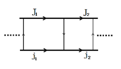
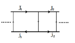
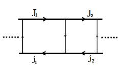
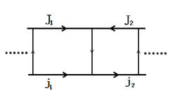
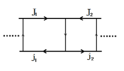
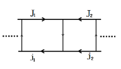
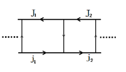
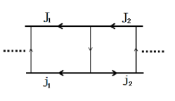
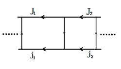
To better understand the properties of our model, we discuss the direction of probability fluxes here. For the special case in which there are only two locations at which the inter-state transition rates are nonzero, i.e., the special case II, there are altogether $18$ different types of probability flux. Since the states 1 and 2 are temporally symmetric, we restrict our discussion only on the cases in which $\omega_{a}P(a)-\omega_{d}\rho(a)\geq 0$ for the continuous model, or $\omega_{a}P_{M}-\omega_{d}\rho_{M}\geq 0$ for the hopping model. Then, there are altogether $9$ different types of probability flux (see Fig. 4). Furthermore, if $\Delta V_{1}=\Delta V_{2}=0$, then there is only one type (see the figure (2, 2) in Fig. 4). On the other hand, if the potential $V_{2}$ is constant (or $f_{i}=b_{i}\equiv f$ for the hopping model), then there are altogether 3 different types of probability flux (see the second column in Fig. 4).

IV Conclusions

In conclusion, two chemical states models of molecular motor are discussed in this paper. For some special cases, explicit expressions of mean velocity are obtained. We find that the mean velocity of molecular motor might not be zero even if both of the potentials are periodic, which means there is no energy input to the molecular motor in each of the chemical states. The energy for the motion molecular motor motion comes from the processes that drive the motor from one state to another. For motor proteins, these processes are ATP hydrolysis. At the same time, from the expression of mean velocity, we find that the velocity of molecular motor might be zero even if there exists nonzero input energy. Which implies that the motion of motor protein is usually loosely coupled to ATP hydrolysis Bieling et al. (2008); Endres et al. (2006); Seidel et al. (2008); Shaevitz et al. (2005); Yildiz et al. (2008); Gao (2006); Nishikawa et al. (2008); Masuda (2009); Gerritsma and Gaspard (2009).

Figure 1: Schematic depiction of two coupled one-dimensional hopping models. In which the forward and backward transition rates of molecular motor in state 1 are denoted by $F_{n}$ and $B_{n}$, and are denoted by $f_{n}$ and $b_{n}$ for molecular motor in state 2, here $1\leq n\leq N$ with $N$ is the period of the hopping models. The inter-state transition rates at position $n$ are denoted by $\omega_{a}^{n}$ (states 1$\to$2) and $\omega_{d}^{n}$ (states 2$\to$1). For motor proteins, $\omega_{a}^{n}$, $\omega_{d}^{n}$ depend on the chemical potentials and concentrations of ATP and ADP.

Figure 2: Special case I of two coupled one-dimensional hopping models. In which $\omega_{a}^{n}=\omega_{d}^{n}=0$ for $1\leq n\leq N-1$, and $\omega_{a}^{N}=\omega_{a}$, $\omega_{d}^{N}=\omega_{d}$. For this special case, the mean velocity of molecular motor would be zero if there is no energy input in each of the two states, i.e., $\Delta G_{1}=\Delta G_{2}=0$. In fact, at steady state, there is also no energy input during the process that drives the motor from one state to another, since $\omega_{a}P_{N}=\omega_{d}\rho_{N}$.

Figure 3: Special case II of two coupled one-dimensional hopping models. In which $\omega_{a}^{n}=\omega_{d}^{n}=0$ for $n\neq M,N$, and $\omega_{a}^{M}=\omega_{a}$, $\omega_{d}^{M}=\omega_{d}$, $\omega_{a}^{N}=\Omega_{a}$, $\omega_{d}^{N}=\Omega_{d}$. For this special case, the mean velocity of molecular motors might not be zero even if there is no energy input in each of the two states, i.e., $\Delta G_{1}=\Delta G_{2}=0$. Since there usually exists energy input to molecular motor during its jump from one state to another unless $\omega_{a}P_{M}=\omega_{d}\rho_{M}$ and $\Omega_{a}P_{N}=\Omega_{d}\rho_{N}$.

Figure 4: Different types of probability flux for special case II. From these figures, one can see that the motion of molecular motors is usually loosely coupled to the energy input process, i.e., there might exist energy input but without directed macroscopic mechanical motion. Part of the input energy will be consumed during substep oscillation.

References

• Bray (2001) D. Bray, Cell movements: from molecules to motility, 2nd Edn (Garland, New York, 2001).
• Howard (2001) J. Howard, Mechanics of Motor Proteins and the Cytoskeleton (Sinauer Associates and Sunderland, MA, 2001).
• Badoual et al. (2002) M. Badoual, F. Jülicher, and J. Prost, Proc. Natl. Acad. Sci. USA 99, 6696 (2002).
• Klumpp and Lipowsky (2005) S. Klumpp and R. Lipowsky, Proc. Natl. Acad. Sci. USA 102, 17284 (2005).
• Riedel-Kruse et al. (2007) I. H. Riedel-Kruse, A. Hilfinger, J. Howard, and F. Jülicher, HFSP J. 1, 192 (2007).
• Zhang (2009a) Y. Zhang, Phys. Rev. E 79, 061918 (2009a).
• Howard (2009) J. Howard, Annu. Rev. Biophys. 38, 217 (2009).
• Vale (2003) R. D. Vale, Cell 112, 467 (2003).
• Fisher and Kolomeisky (2001) M. E. Fisher and A. B. Kolomeisky, Proc. Natl. Acad. Sci. USA 98, 7748 (2001).
• Carter and Cross (2005) N. J. Carter and R. A. Cross, Nature 435, 308 (2005).
• Block (2007) S. M. Block, Biophys. J. 92, 2986 (2007).
• Zhang (2008) Y. Zhang, Biophys. Chem. 136, 19 (2008).
• Toprak et al. (2009) E. Toprak, A. Yildiz, M. T. Hoffman, S. S. Rosenfeld, and P. R. Selvin, Proc. Natl. Acad. Sci. USA 106, 12717 (2009).
• Guydosh and Block (2009) N. R. Guydosh and S. M. Block, Nature 08259 (2009).
• Hyeon et al. (2009) C. Hyeon, S. Klumppb, and J. N. Onuchic, Phys. Chem. Chem. Phys 11, 4899 (2009).
• Hariharan and Hancock (2009) V. Hariharan and W. O. Hancock, Cell. Mol. Bioe. 2, 177 (2009).
• Reck-Peterson et al. (2006) S. L. Reck-Peterson, A. Yildiz, A. P. Carter, A. Gennerich, N. Zhang, and R. D. Vale, Cell 126, 335 (2006).
• Toba et al. (2006) S. Toba, T. M. Watanabe, L. Yamaguchi-Okimoto, Y. Y. Toyoshima, and H. Higuchi, Proc. Natl. Acad. Sci. USA 103, 5741 (2006).
• Gennerich and Vale (2009) A. Gennerich and R. D. Vale, Curr. Opin. Cell. Biol. 21, 59 (2009).
• Houdusse and Carter (2009) A. Houdusse and A. P. Carter, Cell 136, 395 (2009).
• Roberts et al. (2009) A. J. Roberts, N. Numata, M. L. Walker, Y. S. Kato, B. Malkova, T. Kon, R. Ohkura, F. Arisaka, P. J. Knight, K. Sutoh, et al., Cell 136, 485 (2009).
• Kardon et al. (2009) J. R. Kardon, S. L. Reck-Peterson, and R. D. Vale, Proc. Natl. Acad. Sci. USA 106, 5669 (2009).
• Serohijos et al. (2009) A. W. R. Serohijos, W. D. Tsygankov, S. Liu, T. C. Elstonbd, and N. V. Dokholyanz, Phys. Chem. Chem. Phys. 11, 4840 (2009).
• Rosenfeld and Sweeney (2004) S. S. Rosenfeld and H. L. Sweeney, J. Biol. Chem. 279, 40100 (2004).
• Purcell et al. (2005) T. J. Purcell, H. L. Sweeney, and J. A. Spudich, Proc. Natl. Acad. Sci. USA 102, 13873 (2005).
• Veigel et al. (2003) C. Veigel, J. E. Molloy, S. Schmitz, and J. Kendrick-Jones, Nat. Cell. Biol. 5, 980 (2003).
• Sakamoto et al. (2008) T. Sakamoto, M. R. Webb, E. Forgacs, H. D. White, and J. R. Sellers, Nature 455, 128 (2008).
• Del R. Jackson and Baker (2009) J. Del R. Jackson and J. E. Baker, Phys. Chem. Chem. Phys. 11, 4808 (2009).
• Fedorov et al. (2009) R. Fedorov, M. Böhl, G. Tsiavaliaris, F. K. Hartmann, M. H. Taft, P. Baruch, B. Brenner, R. Martin, H.-J. Knölker, H. O. Gutzeit, et al., Nat. Struct. Mol. Biol. 16, 80 (2009).
• Wang and Oster (1998) H. Wang and G. Oster, Nature 396, 279 (1998).
• Kinosita et al. (2000) K. Kinosita, H.Noji, K.Adachi, and R. Yasuda, Phil. Trans. R. Soc. B 355, 473 (2000).
• Nishizaka et al. (2004) T. Nishizaka, K. Oiwa, H. Noji, S. Kimura, E. Muneyuki, M. Yoshida, and K. K. Jr, Nat. Struct. Mol. Biol. 11, 142 (2004).
• Adachi et al. (2007) K. Adachi, K. Oiwa, T. Nishizaka, S. Furuike, H. Noji, H. Itoh, M. Yoshida, and J. K. Kinosita, Cell 130, 309 (2007).
• Muneyuki et al. (2007) E. Muneyuki, T. Watanabe-Nakayama, T. Suzuki, M. Yoshida, T. Nishizaka, and H. Noji, Biophys. J. 92, 1806 (2007).
• Junge et al. (2009) W. Junge, H. Sielaff, and S. Engelbrecht, Nature 459, 364 (2009).
• Jr. et al. (2009) J. H. M. Jr., V. Vajrala, H. L. Infante, J. R.Claycomb, A. Palanisami, J. Fang, and G. T. Mercier, Physica B 404, 503 (2009).
• Block et al. (1990) S. M. Block, L. S. B. Goldstein, and B. J. Schnapp, Nature 348, 348 (1990).
• Yildiz et al. (2004) A. Yildiz, M. Tomishige, R. D. Vale, and P. R. Selvin, Science 303, 676 (2004).
• Asbury et al. (2003) C. L. Asbury, A. N. Fehr, and S. M. Block, Science 302, 2130 (2003).
• Schnitzer and Block (1997) M. J. Schnitzer and S. M. Block, Nature 388, 386 (1997).
• Coy et al. (1999) D. L. Coy, M. Wagenbach, and J. Howard, J. Biol. Chem. 274, 3667 (1999).
• Fehr et al. (2007) A. N. Fehr, C. L. Asbury, and S. M. Block, Biophys. J. (2007).
• Yildiz et al. (2008) A. Yildiz, M. Tomishige, A. Gennerich, and R. D. Vale, Cell 134, 1030 (2008).
• Hackney (2005) D. D. Hackney, Proc. Natl. Acad. Sci. USA 102, 18338 (2005).
• Taniguchi et al. (2005) Y. Taniguchi, M. Nishiyama, Y. Ishhi, and T. Yanagida, Nat. Chem. Biol. 1, 342 (2005).
• Nishiyama et al. (2002) M. Nishiyama, H. Higuchi, and T. Yanagida, Nature Cell Biol. 4, 790 (2002).
• Schnitzer et al. (2000) M. J. Schnitzer, K. Visscher, and S. M. Block, Nat. Cell. Biol. 2, 718 (2000).
• Block et al. (2003) S. M. Block, C. L. Asbury, J. W. Shaevitz, and M. J. Lang, Proc. Natl. Acad. Sci. USA 100, 2351 (2003).
• Gennerich et al. (2007) A. Gennerich, A. P. Carter, S. L. Reck-Peterson, and R. D. Vale, Cell 131, 952 (2007).
• Watanabe and Higuchi (2007) T. M. Watanabe and H. Higuchi, Biophys. J. 92, 4109 (2007).
• Mallik et al. (2004) R. Mallik, B. C. Carter, S. A. Lex, S. J. King, and S. P. Gross, Nature 427, 649 (2004).
• Hirakawa et al. (2000) E. Hirakawa, H. Higuchi, and Y. Y. Toyoshima, Proc. Natl. Acad. Sci. USA 97, 2533 (2000).
• Cho et al. (2008) C. Cho, S. L. Reck-Peterson, and R. D. Vale, J. Biol. Chem. 283, 25839 (2008).
• Ross et al. (2008) J. L. Ross, H. Shuman, E. L. F. Holzbaur, and Y. E. Goldman, Biophys. J. 94, 3115 (2008).
• King and Schroer (2000) S. J. King and T. A. Schroer, Nat. Cell. Biol. 2, 20 (2000).
• Cappello et al. (2007) G. Cappello, P. Pierobon, C. Symonds, L. Busoni, J. C. M. Gebhardt, M. Rief, and J. Prost, Proc. Natl. Acad. Sci. USA 104, 15328 (2007).
• Tsygankov and Fisher (2007) D. Tsygankov and M. E. Fisher, Proc. Natl. Acad. Sci. USA 104, 19321 (2007).
• Gebhardt et al. (2006) J. C. M. Gebhardt, A. E.-M. Clemen, J. Jaud, and M. Rief, Proc. Natl. Acad. Sci. USA 103, 8680 (2006).
• Clemen et al. (2005) A. E.-M. Clemen, M. Vilfan, J. Jaud, J. Zhang, M. Bärmann, and M. Rief, Biophys. J. 88, 4402 (2005).
• Kolomeisky and Fisher (2003) A. B. Kolomeisky and M. E. Fisher, Biophys. J. 84, 1642 (2003).
• Uemura et al. (2004) S. Uemura, H. Higuchi, A. O. Olivares, E. M. D. L. Cruz, and S. Ishiwata, Nat. Struct. Mol. Biol. 11, 877 (2004).
• Oster and Wang (2000) G. Oster and H. Wang, Nature 32, 459 (2000).
• Yardimci et al. (2008) H. Yardimci, M. van Duffelen, Y. Mao, S. S. Rosenfeld, and P. R. Selvin, Proc. Natl. Acad. Sci. USA 105, 6016 (2008).
• Sweeney and Houdusse (2007) H. L. Sweeney and A. Houdusse, Curr. Opin. Cell. Biol. 19, 57 (2007).
• Oguchi et al. (2008) Y. Oguchi, S. V. Mikhailenko, T. Ohki, A. O. Olivares, E. M. D. L. Cruz, and S. Ishiwata, Proc. Natl. Acad. Sci. USA 105, 7714 (2008).
• Bryant et al. (2007) Z. Bryant, D. Altman, and J. A. Spudich, Proc. Natl. Acad. Sci. USA 104, 772 (2007).
• Iwaki et al. (2009) M. Iwaki, A. H. Iwane, T. Shimokawa, R. Cooke, and T. Yanagida, Nat. Chem. Biol. 5, 403 (2009).
• Udovichenko et al. (2002) I. P. Udovichenko, D. Gibbs, and D. S. Williams, J. Cell Sci. 115, 445 (2002).
• Inoue et al. (2002) A. Inoue, J. Saito, R. Ikebe, and M. Ikebe, Nat. Cell. Biol. 4, 302 (2002).
• Tominaga et al. (2003) M. Tominaga, H. Kojima, E. Yokota, H. Orii, R. Nakamori, E. Katayama, M. Anson, T. Shimmen, and K. Oiwa, EMBO J. 22, 1263 (2003).
• Kim et al. (2002) D.-E. Kim, M. Narayan, and S. S. Patel, J. Mol. Biol. 321, 807 (2002).
• Risken (1989) H. Risken, The Fokker-Planck Equation (Springer, Berlin, 1989).
• Zhang (2009b) Y. Zhang, J. Stat. Phys. 134, 669 (2009b).
• Wang and Oster (2002) H. Wang and G. Oster, Europhys. Lett. 57, 134 (2002).
• Gehlen et al. (2008) S. V. Gehlen, M. Evstigneev, and P. Reimann, Phys. Rev. E 77, 031136 (2008).
• Nieuwenhuizen et al. (2004) T. M. Nieuwenhuizen, S. Klumpp, and R. Lipowsky, Phys. A 350, 122 (2004).
• Kolomeisky and Fisher (2007) A. B. Kolomeisky and M. E. Fisher, Ann. Rev. Phys. Chem. 58, 675 (2007).
• Liepelt and Lipowsky (2007) S. Liepelt and R. Lipowsky, Phys. Rev. Lett. 98, 258102 (2007).
• Zhang (2009c) Y. Zhang, Physica A 383, 3465 (2009c).
• Fisher and Kolomeisky (1999) M. E. Fisher and A. B. Kolomeisky, Physica A 274, 241 (1999).
• Reimann et al. (2001) P. Reimann, C. V. den Broeck, H. Linke, P. Hanggi, J. M. Rubi, and A. Pérez-Madrid, Phys. Rev. Lett. 87, 010602 (2001).
• Zhang (2009d) Y. Zhang, Phys. Lett. A 373, 2629 (2009d).
• Pury and Cáceres (2003) P. A. Pury and M. O. Cáceres, J. Phys. A: Math. Gen. 36, 2695 (2003).
• Kolomeisky et al. (2005) A. B. Kolomeisky, E. B. Stukalin, and A. A. Popov, Phys. Rev. E 71, 031902 (2005).
• Bieling et al. (2008) P. Bieling, I. A. Telley, J. Piehler, and T. Surrey, EMBO Reports 19, 1121 (2008).
• Endres et al. (2006) N. F. Endres, C. Yoshioka, R. A. Milligan, and R. D. Vale, Nature 439, 875 (2006).
• Seidel et al. (2008) R. Seidel, J. G. P. Bloom, C. Dekker, and M. D. Szczelkun, EMBO J. 27, 1388 (2008).
• Shaevitz et al. (2005) J. W. Shaevitz, S. M. Block, and M. J. Schnitzer, Biophys. J. 89, 2277 (2005).
• Gao (2006) Y. Q. Gao, Biophys. J. 90, 811 (2006).
• Nishikawa et al. (2008) M. Nishikawa, H. Takagi, T. Shibata, A. H. Iwane, and T. Yanagida, Phys. Rev. Lett. 101, 128103 (2008).
• Masuda (2009) T. Masuda, BioSystems 95, 104 (2009).
• Gerritsma and Gaspard (2009) E. Gerritsma and P. Gaspard, arXiv:0904.4218 (2009).
• Lipowsky (2000) R. Lipowsky, Phys. Rev. Lett. 85, 4401 (2000).
• Lipowsky and Jaster (2003) R. Lipowsky and N. Jaster, J. Stat. Phys. 110, 1141 (2003).
• Chen et al. (1999) Y. Chen, B. Yan, and R. Miura, Phys. Rev. E 60, 3771 (1999).
• Wang et al. (2003) H. Y. Wang, C. S. Peskin, and T. C. Elston, J. theor. Biol. 221, 491 (2003).
• Wang (2004) H. Wang, Int. J. Numer. Anal. Model. 1, 1 (2004).
• Astumian (1997) R. D. Astumian, Science 276, 917 (1997).
• Parmeggiani et al. (1999) A. Parmeggiani, F. Jülicher, A. Ajdari, and J. Prost, Physical Review E 60, 2127 (1999).
• Parrondo and Cisneros (2002) J. M. R. Parrondo and B. J. D. Cisneros, Appl. Phys. A 75, 179 (2002).
• Reimann (2002) P. Reimann, Phys. Rep. 361, 57 (2002).
• Bier and Astumian (1993) M. Bier and R. D. Astumian, Phys. Rev. Lett. 71, 1649 (1993).
• Jülicher and Prost (1995) F. Jülicher and J. Prost, Phys. Rev. Lett. 75, 2618 (1995).
• Prost et al. (1994) J. Prost, J.-F. Chauwin, L. Peliti, and A. Ajdari, Phys. Rev. Lett. 72, 2652 (1994).
• Zhang (2010) Y. Zhang, Chin. J. Chem. Phys. 23, 65 (2010).
• Derrida (1983) B. Derrida, J. Stat. Phys. 31, 433 (1983).
• Qian (1997) H. Qian, Biophys. Chem. 67, 263 (1997).
Refer to caption