Entanglement of Dirac fields in an expanding spacetime

Abstract

We study the entanglement generated between Dirac modes in a 2-dimensional conformally flat Robertson-Walker universe. We find radical qualitative differences between the bosonic and fermionic entanglement generated by the expansion. The particular way in which fermionic fields get entangled encodes more information about the underlying space-time than the bosonic case, thereby allowing us to reconstruct the parameters of the history of the expansion. This highlights the importance of bosonic/fermionic statistics to account for relativistic effects on the entanglement of quantum fields.

I Introduction

The phenomenon of entanglement has been extensively studied in non-relativistic settings. Much of the interest on this quantum property has stemmed from its relevance in quantum information theory. However, relatively little is known about relativistic effects on entanglement Czachor (1997); Peres and Terno (2004); Alsing and Milburn (2003); Terashima and Ueda (2004); Shi (2004); Fuentes-Schuller and Mann (2005); Alsing et al. (2006); Ball et al. (2006a); Adesso et al. (2007); Ling et al. (2007); Ahn et al. (2008); Pan and Jing (2008a); Doukas and Hollenberg (2009); León and Martín-Martínez (2009a); VerSteeg and Menicucci (2009); León and Martín-Martínez (2009b); Moradi (2009); Datta (2009); Lin and Hu (2010); Wang et al. (2010); Martín-Martínez et al. (2010) despite the fact that many of the systems used in the implementation of quantum information involve relativistic systems such as photons. The vast majority of investigations on entanglement assume that the world is flat and non-relativistic. Understanding entanglement in spacetime is ultimately necessary because the world is fundamentally relativistic. Moreover, entanglement plays a prominent role in black hole thermodynamics Bombelli et al. (1986); Mukohyama et al. (1997); Terashima (2000); Emparan (2006); Lévay (2007); Cadoni (2007); Lin and Hu (2008); Fabbri and Navarro-Salas (2005) and in the information loss problem Horowitz and Maldacena (2004); Gottesman and Preskill (2004); Lloyd (2006); Ahn (2006); Ahn et al. (2008); Adesso and Fuentes-Schuller (2009).

Recently, there has been increased interest in understanding entanglement and quantum communication in black hole spacetimes Ge and Kim (2008); Pan and Jing (2008b); Ahn and Kim (2007); Martín-Martínez et al. (2010) and in using quantum information techniques to address questions in gravity Terno (2006); Livine and Terno (2007). Studies on relativistic entanglement show that conceptually important qualitative differences to a non-relativistic treatment arise. For instance, entanglement was found to be an observer-dependent property that is degraded from the perspective of accelerated observers moving in flat spacetime Fuentes-Schuller and Mann (2005); Alsing et al. (2006); León and Martín-Martínez (2009b); Adesso et al. (2007); Mann and Villalba (2009). These results suggest that entanglement in curved spacetime might not be an invariant concept.

In this paper we study the creation of entanglement between Dirac modes due to the expansion of a Robertson-Walker spacetime. A general study of entanglement in curved spacetime is problematic because particle states cannot always be defined in a meaningful way. However, it has been possible to learn about certain aspects of entanglement in curved spacetimes that have asymptotically flat regions Ball et al. (2006b); Adesso and Fuentes-Schuller (2009); Shi (2004); Terashima and Ueda (2004). Such studies show that entanglement can be created by the dynamics of the underlying spacetime Ball et al. (2006b); VerSteeg and Menicucci (2009) as well as destroyed by the loss of information in the presence of a spacetime horizon Fuentes-Schuller and Mann (2005); Adesso and Fuentes-Schuller (2009); Martín-Martínez et al. (2010).

Such investigations not only deepen our understanding of entanglement but also offer the prospect of employing entanglement as a tool to learn about curved spacetime. For example, the entanglement generated between bosonic modes due to the expansion of a model 2-dimensional universe was shown to contain information about its history Ball et al. (2006b), affording the possibility of deducing cosmological parameters of the underlying spacetime from the entanglement. This novel way of obtaining information about cosmological parameters could provide new insight into the early universe both theoretically (incorporating into cosmology entanglement as a purely quantum effect produced by gravitational interactions in an expanding universe) and experimentally (either by development of methods to measure entanglement between modes of the background fields or by measuring entanglement creation in condensed matter analogs of expanding space-time Uhlmann et al. (2005); Jain et al. (2007)). Other interesting results show that entanglement plays a role in the thermodynamic properties of Robertson-Walker type spacetimes Müller and Lousto (1995) and can in principle be used to distinguish between different spacetimes VerSteeg and Menicucci (2009) and probe spacetime fluctuations Han et al. (2008).

Here we consider entanglement between modes of a Dirac field in a 2-dimensional Robertson-Walker universe. We find that the entanglement generated by the expansion of the universe for the same fixed conditions is lower than for the bosonic case Ball et al. (2006b). However we also find that fermionic entanglement codifies more information about the underlying spacetime structure. These contrasts are commensurate with the flat spacetime case, in which entanglement in fermionic systems was found to be more robust against acceleration than that in bosonic systems Alsing et al. (2006); León and Martín-Martínez (2009b). In the limit of infinite acceleration fermionic entanglement remains finite due to statistical effects Martín-Martínez and León (2009, 2010) which resemble those found in first quantization scenarios Schliemann et al. (2001).

Our paper is organized as follows: In section II we revise the Dirac equation in a spatially flat $d$-dimensional Robertson-Walker universe. Subsequently setting $d=2$, in section III we calculate the entanglement entropy of two Dirac modes and compare it with the bosonic case. In section IV we explain the origin of the entanglement peculiarities of the fermionic case, showing how it can give us more information about the parameters of the expansion. Conclusions are presented in section V.

II Dirac field in a $d$-dimensional Robertson-Walker universe

As we mentioned before, entanglement between modes of a quantum field in curved spacetime can be investigated in special cases where the spacetime has at least two asymptotically flat regions. Such is the case of the Robertson-Walker universe where spacetime is flat in the distant past and in the far future. In this section, following the work done by Bernard and Duncan Bernard and Duncan (1977); Duncan (1978), we find the state of a Dirac field in the far future that corresponds to a vacuum state in the remote past.

Consider a Dirac field $\psi$ with mass $m$ on a $d$-dimensional spatially flat Robertson-Walker spacetime with line element,

$$ds^{2}=C(\eta)(-d\eta^{2}+dx_{i}dx^{i}).$$ (1)

$x_{i}$ are the spacial coordinates and the temporal coordinate $\eta$ is called the conformal time to distinguish it from the cosmological time $t$. The metric is conformally flat, as are all Robertson-Walker metrics. The dynamics of the field is given by the covariant form of the Dirac equation on a curved background,

$$\{i\gamma^{\mu}(\partial_{\mu}-\Gamma_{\mu})+m\}\psi=0,$$ (2)

where $\gamma^{\mu}$ are the curved Dirac-Pauli matrices and $\Gamma_{\mu}$ are spinorial affine connections. The curved Dirac-Pauli matrices satisfy the condition,

$$\gamma^{\mu}\gamma^{\nu}+\gamma^{\nu}\gamma^{\mu}=2g^{\mu\nu},$$ (3)

where $g^{\mu\nu}$ is the spacetime metric. In the flat case where the metric is given by $\eta^{\alpha\beta}$, the constant special relativistic matrices are defined by,

$$\bar{\gamma}^{\alpha}\bar{\gamma}^{\beta}+\bar{\gamma}^{\beta}\bar{\gamma}^{\alpha}=2\eta^{\alpha\beta}.$$ (4)

The relation between curved and flat ${\gamma}$ matrices is given by $\gamma_{\mu}=e_{\mu}^{\;\;\alpha}\bar{\gamma}_{\alpha}$ where $e_{\mu}^{\;\;\alpha}$ is the vierbein (tetrad) field satisfying the relation $e_{\mu}^{\;\;\alpha}e_{\nu}^{\;\;\beta}\eta_{\alpha\beta}=g_{\mu\nu}$.

In order to find the solutions to the Dirac equation Eq. (2) on this spacetime, we note that $C(\eta)$ is independent of x. We exploit the resulting spatial translational invariance and separate the solutions into

$$\psi_{k}(\eta,x)=e^{i\bm{k\cdot x}}C^{(1-d)/4}\left(\bar{\gamma}^{0}\partial_{\eta}+i\bar{\bm{\gamma}}\cdot{{\bm{k}}}-mC^{1/2}\right)\phi_{k}(\eta),$$ (5)

where $k^{2}=|{{\bm{k}}}|^{2}=\sum_{i=1}^{d-1}k_{i}^{2}$. Inserting this into the Dirac equation, we obtain the following coupled equations

$$\left(\partial_{\eta}^{2}+m^{2}C\pm im\dot{C}C^{-1/2}+|{{\bm{k}}}|^{2}\right)\phi_{k}^{(\pm)}=0,$$ (6)

using the fact that the eigenvalues of $\bar{\gamma}^{0}$ are $\pm 1$. In order to quantize the field and express it in terms of creation and annihilation operators, positive and negative frequency modes must be identified. This cannot be done globally. However positive and negative frequency modes can be identified in the far past and future where the spacetime admits timelike killing vector fields $\pm\partial/\partial\eta$. Provided $C(\eta)$ is constant in the far past $\eta\rightarrow-\infty$ and far future $\eta\rightarrow+\infty$, the asymptotic solutions of Eq. (6) will be $\phi^{(\pm)}_{in}\sim e^{\pm i\omega_{in}\eta}$ and $\phi^{(\pm)}_{out}\sim e^{\pm i\omega_{out}\eta}$ respectively, where

$$\omega_{in} = (|{\bm{k}}|^{2}+\mu_{in}^{2})^{1/2}$$ (7)

$$\omega_{out} = (|{\bm{k}}|^{2}+\mu_{out}^{2})^{1/2}$$

$$\mu_{in} = m\sqrt{C(-\infty)},$$

$$\mu_{out} = m\sqrt{C(+\infty)}.$$

The action of the Killing vector field on the asymptotic solutions allow us to identify $\phi^{(\mp)\ast}_{in}$ and $\phi^{(\mp)\ast}_{out}$ as negative frequency solutions. The sign flip is due to the explicit factor $i$ in (6). A consequence of the linear transformation properties of such functions is that the Bogolubov transformations associated with the transformation between $in$ and $out$ solutions take the simple form Duncan (1978)

$$\phi_{in}^{(\pm)}(k)=\alpha_{k}^{(\pm)}\phi^{(\pm)}_{out}(k)+\beta_{k}^{(\pm)}\phi^{(\mp)*}_{out}(k),$$ (8)

where $\alpha^{\pm}_{k}$ and $\beta^{\pm}_{k}$ are Bogoliubov coefficients.

The curved-space spinor solutions of the Dirac equation are defined by (with corresponding $U_{out}$, $V_{out}$ and $K_{out}$),

$$U_{in}(\bm{k},\lambda;x,\eta)\!\! \equiv \!\!K_{in}(k)[C(\eta)]^{(1-d)/4}\Big{[}-i\partial_{\eta}+i{\bm{k}}\cdot\bar{\gamma}$$

$$\!\!-m\sqrt{C(\eta)}\Big{]}\phi_{k}^{in(-)(\eta)}e^{i\bm{k}\cdot{\bm{x}}}u(0,\lambda)$$

$$V_{in}(\bm{k},\lambda;x,\eta)\!\! \equiv \!\!K_{in}(k)[C(\eta)]^{(1-d)/4}\Big{[}i\partial_{\eta}-i{\bm{k}}\cdot\bar{\gamma}$$

$$\!\!-m\sqrt{C(\eta)}\Big{]}\phi_{k}^{in(+)\ast(\eta)}e^{-i\bm{k}\cdot{\bm{x}}}v(0,\lambda),$$

where $K_{in}\equiv-(1/|k|)((\omega_{in}-\mu_{in})/2\mu_{in})^{1/2}$ and $u(0,\lambda)$, $v(0,\lambda)$ are flat space spinors satisfying,

$$\gamma^{0}u(0,\lambda) = -iu(0,\lambda),$$

$$\gamma^{0}v(0,\lambda) = iv(0,\lambda),$$

for $1\leq\lambda\leq 2^{d/2-1}$. The field in the “in” region can then be expanded as,

$$\psi(x) = \frac{1}{\sqrt{(2\pi)^{1-d}}}\int d^{d-1}k\left[\frac{\mu_{in}}{\omega_{in}}\right]\sum_{\lambda=1}^{d/2-1}\big{[}a_{in}({\bm{k}},\lambda)$$ (10)

$$U_{in}({\bm{k}},\lambda;\bm{x},\eta)+b^{{\dagger}}_{in}({\bm{k}},\lambda)V_{in}({\bm{k}},\lambda;\bm{x},\eta)\big{]}$$

with a similar expression for the “out” region. The $in$ and $out$ creation and annihilation operators for particles and anti-particles obey the usual anticommutation relations. Using the Bogoliubov transformation one can expand the $out$ operators in terms of $in$ operators

$$a_{out}(\bm{k},\lambda) = \left(\frac{\mu_{in}\omega_{out}}{\omega_{in}\mu_{out}}\right)^{\frac{1}{2}}\frac{K_{in}}{K_{out}}\Bigg{(}\alpha_{k}^{(-)}a_{in}(\bm{k},\lambda)$$ (11)

$$+ \beta_{k}^{(-)\ast}\sum_{\lambda^{\prime}}X_{\lambda\lambda^{\prime}}(-{\bm{k}})b^{{\dagger}}_{in}(-{\bm{k}},\lambda^{\prime})\Bigg{)},$$

$$b_{out}(\bm{k},\lambda) = \left(\frac{\mu_{in}\omega_{out}}{\omega_{in}\mu_{out}}\right)^{\frac{1}{2}}\frac{K_{in}}{K_{out}}\Bigg{(}\alpha_{k}^{(-)}b_{in}(\bm{k},\lambda)$$ (12)

$$+ \beta_{k}^{(-)\ast}\sum_{\lambda^{\prime}}X_{\lambda\lambda^{\prime}}(-{\bm{k}})a^{{\dagger}}_{in}(-{\bm{k}},\lambda^{\prime})\Bigg{)},$$

where

$$X_{\lambda\lambda^{\prime}}(-{\bm{k}})=-2\mu_{out}^{2}K^{2}_{out}\bar{u}_{out}(-{\bm{k}},\lambda^{\prime})v(0,\lambda).$$ (13)

and

$$K_{in/out}=\frac{1}{|k|}\left(\frac{\omega_{in/out}(k)-\mu_{in/out}}{\mu_{in/out}}\right)^{1/2}.$$ (14)

This yields the following relationship between Bogoliubov coefficients,

$$\left|\alpha^{(-)}_{k}\right|^{2}\!\!\!-2\mu_{out}^{2}K_{out}^{2}\left(1-\frac{\omega_{out}}{\mu_{out}}\right)\!\!\left|\beta_{k}^{(-)}\right|^{2}\!\!\!\!=\!\frac{\mu_{out}}{\mu_{in}}\frac{\omega_{in}}{\omega_{out}}\!\left(\frac{K_{out}}{K_{in}}\right)^{2}\!\!\!\!.$$ (15)

We consider the special solvable case presented in Duncan (1978) $C(\eta)=(1+\epsilon(1+\tanh\rho\eta))^{2}$, where $\epsilon,\rho$ are positive real parameters controlling the total volume and rapidity of the expansion, respectively. In this case the solutions of the Dirac equation that in remote past reduce to positive frequency modes are,

$$\phi^{(\pm)}_{in} = \exp\left(-i\omega_{+}\eta-\frac{i\omega_{-}}{\rho}\ln[2\cosh\rho\eta]\right)$$

$$\!\!\!\!\!\!\!\!\!\!\!\!\!\!\!\!\!\!\!\!\!\!\!\times F_{1}\!\left(\!1\!+\!\frac{i(\omega_{-}\!\pm m\epsilon)}{\rho},\frac{i(\omega_{-}\!\mp m\epsilon)}{\rho},1\!-\!\frac{i\omega_{in}}{\rho},\frac{1\!+\!\tanh(\rho\eta)}{2}\!\right)\!\!,$$

where $F_{1}$ is the ordinary hypergeometric function. Similarly, one may find a complete set of modes of the field that behaving as positive and negative frequency modes in the far future,

$$\phi^{(\pm)}_{out} = \exp\left(-i\omega_{+}\eta-\frac{i\omega_{-}}{\rho}\ln[2\cosh\rho\eta]\right)$$

$$\!\!\!\!\!\!\!\!\!\!\!\!\!\!\!\!\!\!\!\!\!\!\!\!\times F_{1}\!\left(\!1\!+\!\frac{i(\omega_{-}\!\pm m\epsilon)}{\rho},\frac{i(\omega_{-}\!\mp m\epsilon)}{\rho},\!1\!+\!\frac{i\omega_{out}}{\rho},\frac{1\!-\!\tanh(\rho\eta)}{2}\!\right)\!\!,$$

where $\omega_{\pm}=(\omega_{out}\pm\omega_{in})/2$. The spacetime obtained by considering this special form of $C(\eta)$ was introduced by Duncan Duncan (1978). It is easy to see that it corresponds to a Minkowskian spacetime in the far future and past, i.e., $C\rightarrow(1+2\epsilon)^{2}$ in the $out$ region and $C\rightarrow 1$ at the $in$ region.

If we define $|\gamma^{-}|^{2}\equiv\left|\beta^{(-)}_{k}/\alpha^{(-)}_{k}\right|^{2}$, for this spacetime we get that

$$\left|\gamma^{-}\right|^{2} = \frac{(\omega_{-}+m\epsilon)(\omega_{+}+m\epsilon)}{(\omega_{-}-m\epsilon)(\omega_{+}-m\epsilon)}$$ (16)

$$\times \!\!\frac{\sinh\left[\frac{\pi}{\rho}(\omega_{-}-m\epsilon)\right]\sinh\left[\frac{\pi}{\rho}(\omega_{-}+m\epsilon)\right]}{\sinh\left[\frac{\pi}{\rho}(\omega_{+}+m\epsilon)\right]\sinh\left[\frac{\pi}{\rho}(\omega_{+}-m\epsilon)\right]}$$

An analogous procedure can be followed for scalar fields Ball et al. (2006b). The time dependent Klein-Gordon equation in this spacetime is given by

$$\left(\partial_{\eta}^{2}+k^{2}+C(\eta)m^{2}\right)\chi_{k}(\eta)=0.$$ (17)

After some algebra, the solutions of Klein-Gordon equation behaving as positive frequency modes as $\eta\rightarrow-\infty(t\rightarrow-\infty)$, are found to be

$$\chi_{in}(\eta) = \exp\left(-i\omega_{+}\eta-\frac{i\omega_{-}}{\rho}\ln[2\cosh\rho\eta]\right)$$

$$\!\!\!\!\!\!\!\!\!\!\!\!\!\!\!\!\!\!\!\!\!\!\!\!\!\!\!\!\times F\!\left(\frac{1}{2}\!-\!\frac{i\bar{\omega}}{2\rho}\!+\!\frac{i\omega_{-}}{\rho},\frac{1}{2}\!+\!\frac{i\bar{\omega}}{2\rho}\!+\!\frac{i\omega_{-}}{\rho},1\!-\!i\frac{\omega_{in}}{\rho},\frac{1\!+\!\tanh(\rho\eta)}{2}\!\right)\!.$$

Similarly we have

$$\chi_{out}(\eta) = \exp\left(-i\omega_{+}\eta-\frac{i\omega_{-}}{\rho}\ln[2\cosh\rho\eta]\right)$$

$$\!\!\!\!\!\!\!\!\!\!\!\!\!\!\!\!\!\!\!\!\!\!\!\!\!\!\!\!\!\!\times F\!\left(\frac{1}{2}\!-\!\frac{i\bar{\omega}}{2\rho}\!+\!\frac{i\omega_{-}}{\rho},\frac{1}{2}\!+\!\frac{i\bar{\omega}}{2\rho}\!+\!\frac{i\omega_{-}}{\rho},1\!-\!i\frac{\omega_{out}}{\rho},\frac{1\!-\!\tanh(\rho\eta)}{2}\!\right)\!.$$

where $\bar{\omega}=(m^{2}(2\epsilon+1)^{2}-\rho^{2})^{1/2}$. Computing the quotient of the Bogoliubov coefficients for this bosonic case, we find

$$|\gamma_{B}^{-}|^{2}=\frac{\cosh\frac{\pi}{\rho}\bar{\omega}+\cosh\frac{2\pi}{\rho}\omega_{-}}{\cosh\frac{\pi}{\rho}\bar{\omega}+\cosh\frac{2\pi}{\rho}\omega_{+}}.$$ (18)

III Entanglement generated due to the expansion of the universe

It is then possible to find the state in the far future that corresponds to the vacuum state in the far past. By doing that we will show that the vacuum state of the field in the asymptotic past evolves to an entangled state in the asymptotic future. The entanglement generated by the expansion codifies information about the parameters of the expansion, this information is more easily obtained from fermionic fields than bosonic, as we will show below.

Since we want to study fundamental behaviour we will consider the 2-dimensional case, which has all the fundamental features of the higher dimensional settings.

Using the relationship between particle operators in asymptotic times,

$$b_{in}(k)=\left[{\alpha^{-}_{k}}^{\ast}b_{out}(k)+{\beta^{-}_{k}}^{\ast}\chi(k)a_{out}^{\dagger}(-k)\right],$$ (19)

we can obtain the asymptotically past vacuum state in terms of the asymptotically future Fock basis. Demanding that $b_{in}(\bar{k},\lambda)|0\rangle_{in}=0$ we can find the “in” vacuum in terms of the “out” modes. Due to the form of the Bogoliubov transformations the “in” vacuum must be of the form

$$|0\rangle_{in}=\prod_{k}(A_{0}|0\rangle_{out}+A_{1}|1_{k}1_{-k}\rangle_{out})$$

where to compress notation $|1_{-k}\rangle$ represents an antiparticle mode with momentum $-k$ and $|1_{k}\rangle$ a particle mode with momentum $k$. Here we wrote the state for each frequency in the Schmidt decomposition. Since different $k$ do not mix it is enough to consider only one frequency. Imposing $b_{in}(\bar{k})|0\rangle_{in}=0$ we obtain the following condition on the vacuum coefficients

$${\alpha^{-}_{k}}^{*}A_{1}|1_{-k}\rangle+{\beta^{-}_{k}}^{*}\chi(\bar{k})A_{0}|1_{-k}\rangle=0$$ (20)

giving

$$A_{1}=-\frac{{\beta^{-}_{k}}^{*}}{{\alpha^{-}_{k}}^{*}}\chi(\bar{k})A_{0}=-\gamma^{-\ast}\chi(\bar{k})A_{0}$$ (21)

where

$$\gamma^{-\ast}({k})=\frac{{\beta^{-}_{k}}^{*}}{{\alpha^{-}_{k}}^{*}}$$ (22)

From the vacuum normalization,

$$1 = {}_{in}\langle 0|0\rangle_{in}=|A_{0}|^{2}(1+|\gamma^{-}({k})\chi(\bar{k})|^{2}).$$ (23)

Therefore, the vacuum state

$$|0\rangle_{in}=\prod_{k}\frac{|0\rangle_{out}-\gamma^{-\ast}({k})\chi(\bar{k})|1_{k}1_{-k}\rangle_{out}}{\sqrt{1+|\gamma^{-}({k})\chi(\bar{k})|^{2}}}$$ (24)

is an entangled state of particle modes and antiparticle modes with opposite momenta.

Since the state is pure, the entanglement is quantified by the von-Neumann entropy given by $S(\rho_{k})=\mathrm{Tr}(\rho_{k}\log_{2}\rho_{k})$ where $\rho_{k}$ is the reduced density matrix of the state for mode $k$. Tracing over the antiparticle modes with momentum $-k$ (or alternatively, particle modes with momentum $k$) we obtain

$$\rho_{k}=\frac{1}{(1+|\gamma_{k}^{-}\chi(\bar{k})|^{2})}(|0\rangle\langle 0|+|\gamma_{k}^{-\ast}({k})\chi(\bar{k})|^{2}|1_{k}\rangle\langle 1_{k}|).$$ (25)

The von Neumann entropy of this state is simply

$$S(\rho_{k})=\log(1+|\gamma_{k}^{-}\chi(\bar{k})|^{2})-\frac{|\gamma_{k}^{-\ast}\chi(\bar{k})|^{2}\log(|\gamma_{k}^{-\ast}\chi(\bar{k})|^{2})}{(1+|\gamma_{k}^{-}\chi(\bar{k})|^{2})}$$ (26)

Using the following identity

$$|\chi_{\lambda\lambda}|^{2}=2\mu_{out}K^{2}_{out}(\mu_{out}-\omega_{out})=\left[\frac{\mu_{out}}{|k|}\left(1-\frac{\omega_{out}}{\mu_{out}}\right)\right]^{2}$$ (27)

we obtain the entanglement entropy

$$S(\rho_{k}) = \log\left(1+\frac{\mu^{2}_{out}}{|k|^{2}}\left(1-\frac{\omega_{out}}{\mu_{out}}\right)^{2}|\gamma_{k}^{-}|^{2}\right)$$ (28)

$$- \frac{\frac{\mu^{2}_{out}}{|k|^{2}}\left(1-\frac{\omega_{out}}{\mu_{out}}\right)^{2}|\gamma_{k}^{-\ast}|^{2}}{(1+\frac{\mu^{2}_{out}}{|k|^{2}}\left(1-\frac{\omega_{out}}{\mu_{out}}\right)^{2}|\gamma_{k}^{-}|^{2})}$$

$$\times \log\left(\frac{\mu^{2}_{out}}{|k|^{2}}\left(1-\frac{\omega_{out}}{\mu_{out}}\right)^{2}|\gamma_{k}^{-\ast}(\bar{k})|^{2}\right)$$

Using (28) we find that the fermionic entanglement is

$$S_{F}=\log\left(\frac{1+|\gamma_{F}^{-}|^{2}}{|\gamma_{F}^{-}|^{\frac{2|\gamma_{F}^{-}|^{2}}{|\gamma_{F}^{-}|^{2}+1}}}\right)$$ (29)

where $|\gamma_{F}|=|\gamma_{k}^{-}\chi(\bar{k})|$. Note that for massless fields ($m=0$) the entanglement vanishes since $\omega_{-}=0$ and $\gamma^{-}$=0. Comparing our result to the bosonic case studied in Ball et al. (2006b) we find

$$S_{B}=\log\left(\frac{|\gamma_{B}^{-}|^{\frac{2|\gamma_{B}^{-}|^{2}}{|\gamma_{B}^{-}|^{2}-1}}}{1-|\gamma_{B}|^{2}}\right)$$ (30)

where the expression for $\gamma_{B}$ in (18) differs from that in ref. Ball et al. (2006b) due to the different scale factor used.

The difference between the bosonic and fermionic cases means that the response of entanglement to the dynamics of the expansion of the universe depends on the nature of the quantum field. We see from (24) that each fermionic field mode is always in a qubit state (the exclusion principle imposes a dimension-2 Hilbert space for the partial state). However in the bosonic case Ball et al. (2006b) the Hilbert space for each mode is of infinite dimension, as every occupation number state of the $out$ Fock basis participates in the $in$ vacuum. In both cases the entanglement increases monotonically with the expansion rate $\rho$ and the total volume expansion parameter $\epsilon$. It is possible to find analytically the asymptotic values that both fermionic and bosonic entanglement reach at infinity. For example, when $k=m=\rho=1$ we find that as $\epsilon\rightarrow\infty$

$$\gamma_{B}^{-}\to e^{-\pi\sqrt{2}}\qquad\gamma_{F}\to e^{-\pi\sqrt{2}}\frac{e^{\pi\sqrt{2}}-e^{\pi}}{e^{\pi\sqrt{2}+1}-1}$$ (31)

respectively yielding

$$S_{B}(\epsilon\rightarrow\infty)\approx 0.0913\qquad S_{F}(\epsilon\rightarrow\infty)\approx 0.0048$$ (32)

The entanglement entropy is bounded by $S_{E}<\log_{2}N$ where $N$ is the Hilbert space dimension of the partial state. The fermionic upper limit $S_{E}=1$ corresponds to a maximally entangled state. For bosons the unbounded dimension of the Hilbert space implies the entropy of entanglement is not bounded by unity Ball et al. (2006b). However this distinction does not guarantee that we can extract more information from bosons as we shall now demonstrate.

IV Fermionic entanglement and the expansion of the universe

As seen in figures 1 and 2 the entanglement behaviour is completely different for bosons (fig. 1) and fermions (fig. 2). Although the behaviour as the mass of the field varies seems qualitatively similar, the variation with the frequency of the mode is completely different.

The entanglement dependence on $|\bm{k}|$ for bosons is monotonically decreasing whereas for fermions, the global space-time structure ‘selects’ one value of $|\bm{k}|$ for which the expansion of the space-time generates a larger amount of entanglement (peak in figure 2). We shall see that this selection of a privileged mode is sensitive to the expansion parameters. This may be related to the fermionic nature of the field insofar as the exclusion principle impedes entanglement for too small $|\bm{k}|$.

Regardless of its origin, we can take advantage of this special behaviour for fermionic fields to use the expansion-generated entanglement to engineer a method to obtain information about the underlying space-time more efficiently than for bosons.

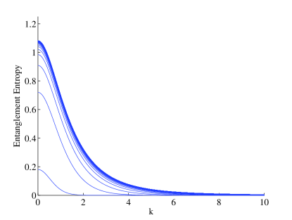
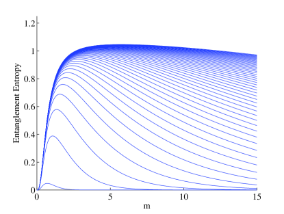
Figure 1: Bosonic field: $S_{E}$ for a fixed mass $m=1$ as a funciton of $|\bm{k}|$ (up) and for a fixed $|\bm{k}|=1$ as a function of $m$ (down) for different rapidities $\rho=1,\dots,100$. An asymptotic regime is reached when $\rho\rightarrow\infty$. $\epsilon$ is fixed $\epsilon=1$

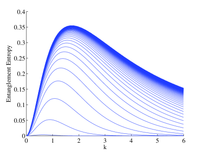
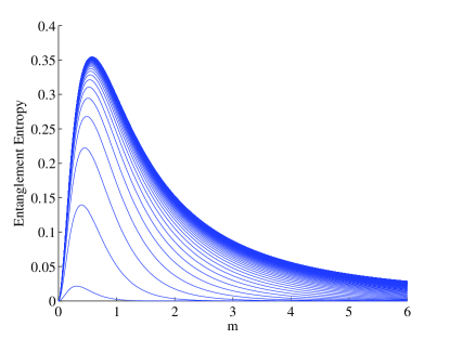
Figure 2: Fermionic field: $S_{E}$ for a fixed mass $m=1$ as a funciton of $|\bm{k}|$ (up) and for a fixed $|\bm{k}|=1$ as a function of $m$ (down) for different rapidities $\rho=1,\dots,100$. The maximum shifts to the right reaching an asymptotic value as $\rho\rightarrow\infty$. $\epsilon$ is fixed $\epsilon=1$. The behaviour as $|\bm{k}|$ varies is radically different from the bosonic case.

IV.1 Using fermionic fields to extract information from the ST structure

Doing a conjoint analysis of the mass and momentum dependence of the entropy we can exploit the characteristic peak that $S_{E}(m,|\bm{k}|)$ presents for fermionic fields to obtain information from the underlying structure of the space-time better than we can do with a bosonic field. Let us first show both dependences simultaneously. Figure 3 shows the entropy of entanglement as a function of our field parameters ($|\bm{k}|$ and mass) for different values of the rapidity.

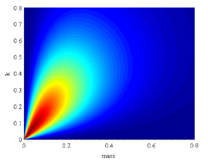
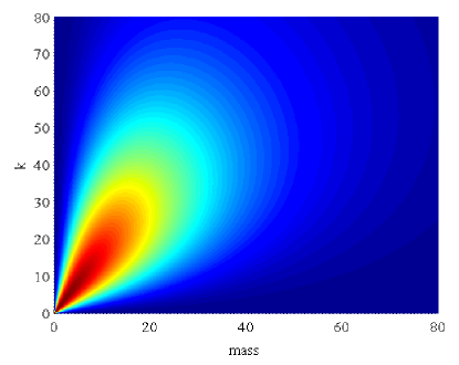
Figure 3: (Color online) $S_{E}(m,|\bm{k}|)$ for $\epsilon=1$, $\rho=1$ (up) $\rho=100$ (down). Red color $\equiv$ higher $S_{E}(m,|\bm{k}|)$

We see from figure 3 that there is no saturation as $\rho\rightarrow\infty$. Instead, as $\rho$ is increased the plot is just rescaled. This is crucial in order to be able to trace back the metric parameters from entanglement creation. We also see from figure 3 that, for a given field mass, there is an optimal value of $|\bm{k}|$ that maximises the entropy. In figure 4 we represent this optimal $|\bm{k}|$ as a function of the mass for different values of $\rho$, showing how the mode which get most entangled as a result of the spacetime expansion changes with the mass field for different rapidities.

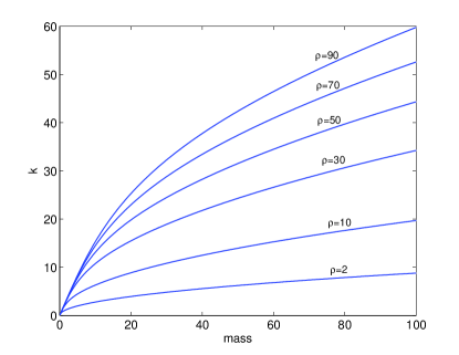
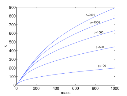
Figure 4: $\epsilon=1$, optimal $|\bm{k}|$ curves (maximum entanglement mode) as a function of the field mass for $\rho=10,\dots,2000$

From the figure we can readily notice two important features

• The optimal $|\bm{k}|$ curve is very sensitive to $\rho$ variations and there is no saturation (no accumulation of these lines) as $\rho$ is increased.

• There is always a field mass for which the optimal $|\bm{k}|$ clearly distinguishes arbitrarily large values of $\rho$.

In figure 5 we can see a consequence of the re-scaling (instead of saturation) of $S_{E}(m,|\bm{k}|)$ when $\rho$ varies. In this figure we show simultaneously the entropy in the optimal curve and the value of the optimal $|\bm{k}|$ as a function of the mass of the field for two different values of $\rho$, showing that if $\rho$ results to be very large, entanglement decays more slowly for higher masses.

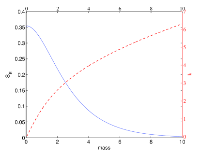
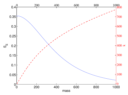
Figure 5: (Color online) $S_{E}$ (blue continuous line) and $k$ (red dashed line) in the line of optimal $k$ as a function of mass for $\rho=10$ (up) and $\rho=1500$ (down). $\epsilon$ is fixed $\epsilon=1$

The relationship between mass and the optimal frequency is very sensitive to variations in $\rho$, presenting no saturation. Conversely figure 6 shows that the optimal $|\bm{k}|$ curve is almost completely insensitive to $\epsilon$.

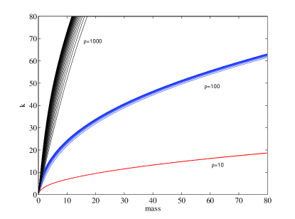
Figure 6: (Color online) Optimal $|\bm{k}|$ as a function of the mass of the field for different vlues of $\epsilon=6,9,12,\dots,99$ and $\rho=10,100,1000$ showing rapid saturation in $\epsilon$. For higher $\epsilon$ this curves are completely insensitive to $\epsilon$ variations, being very little sensitive for smaller values $\epsilon<10$

All the different $\epsilon$ curves are very close to each other. We can take advantage of this to estimate the rapidity independently of the value of $\epsilon$ using the entanglement induced by the expansion on fermionic fields.

IV.2 Optimal $|k|$ tuning method

IV.2.1 Part I: Rapidity estimation protocol

Given a field of fixed mass, we obtain the entanglement for different modes $k_{1},\dots,k_{n}$ of the field. Then the mode $k_{i}$ that returns the maximum entropy will codify information about the rapidity $\rho$, as seen in figure 4. One advantage of this method is that there is no need to assume a fixed $\epsilon$ to estimate $\rho$, since the tuning curves (fig. 4) are have low sensitivity to $\epsilon$ (fig. 6). Furthermore this method does not saturate for higher values of $\rho$ since we can use heavier fields to overcome the saturation observed in figure 2. While one might expect that heavier masses would mean smaller maximum entropy, figure 5 shows that if $\rho$ is high enough to force us to look at heavier fields to improve its estimation, the amount of entanglement will also be high enough due to the scaling properties of $S_{E}(|\bm{k}|,m)$. We can therefore safely use more massive fields to do estimate $\rho$ since they better codify its value.

Hence we have a method for extracting information about $\rho$ that is not affected by the value of $\epsilon$. Information about $\rho$ is quite clearly encoded in the optimal $|\bm{k}|$ curve, which is a direct consequence of the peaked behaviour of $S_{E}(|\bm{k}|,m)$.

IV.2.2 Part II: Lower bound for $\epsilon$ via optimal $|k|$ tuning

We can see from figure 4 that for different values of $\rho$ the maximum value for the entanglement at the optimal point (optimal $k$ and optimal $m$) is always $S_{E}^{\text{max}}\approx 0.35$. Consider now $\epsilon\neq 1$. In figure 7 we can see how the maximum entanglement that can be achieved for optimal frequency and mass varies with the volume parameter $\epsilon$. Indeed, the maximum possible entanglement that the optimal mode can achieve is a function of only $\epsilon$ and is independent of $\rho$.

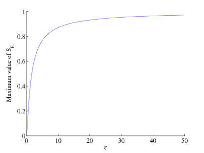
Figure 7: $S_{E}^{\text{max}}(\epsilon)$: Maximum entanglement achievable (optimal $m$ and $|\bm{k}|$) as a function of $\epsilon$. It does not depend at all on $\rho$

Hence information about $\epsilon$ is encoded in the maximum achievable fermionic entanglement. Consequently we can find a method for obtaining a lower bound for the total volume of the expansion of the space-time regardless of the value of the rapidity.

In this fashion we obtain a lower bound for $\epsilon$ since the entanglement measured for the optimal mode is never larger than the maximum achievable entanglement represented in figure 7, $S_{E}(|\bm{k}|,m)\leq S_{E}^{\text{max}}$. For instance if the entanglement in the optimal mode is $S_{E}>0.35$ this will tell us that $\epsilon>1$, whereas if $S_{E}>0.87$ then we can infer that $\epsilon>10$. Note that as $\epsilon$ increases the entanglement in the optimal $|k|$ mode for the optimal mass field approaches that of a maximally entangled state when $\epsilon\rightarrow\infty$ .

Although this method presents saturation when $\epsilon\rightarrow\infty$ (being most effective for $\epsilon\leq 20$) its insensitivity to $\bm{\rho}$ means that the optimal $|\bm{k}|$ method gives us two independent methods for estimating $\rho$ and $\epsilon$. In other words, all the information about the parameters of the expansion (both volume and rapidity) is encoded in the entanglement for the optimal frequency $|\bm{k}|$.

IV.3 Interpretation for the dependence of $S_{E}$ on $|{\bm{k}}|$

We have seen (figure 1) that for bosons a monotonically decreasing entanglement is observed as $|\bm{k}|$ increases. By contrast, in the fermionic case we see that there are privileged $|\bm{k}|$ for which entanglement creation is maximum. These modes are far more prone to entanglement than any others.

To interpret this we can regard the optimal value of $|\bm{k}|$ as being associated with a characteristic wavelength (proportional to $|\bm{k}|^{-1}$) that is increasingly correlated with the characteristic length of the universe. As $\rho$ increases the peak of the entanglement entropy shifts towards higher $|\bm{k}|$, with smaller characteristic lengths. Intuitively, fermion modes with higher characteristic lengths are less sensitive to the underlying space-time because the exclusion principle impedes the excitation of ‘very long’ modes (those whose $|\bm{k}|\rightarrow 0$).

What about small $|\bm{k}|$ modes? As shown in Ball et al. (2006b) and in figure 1, for bosons the entanglement generation is higher when $|\bm{k}|\rightarrow 0$. This makes sense because modes of smaller $|\bm{k}|$ are more easily excited as the space-time expands (it is energetically much ‘cheaper’ to excite smaller $|\bm{k}|$ modes). For fermions entanglement generation, somewhat counterintuitively, decreases for $|\bm{k}|\rightarrow 0$. However if we naively think of fermionic and bosonic excitations in a box we can appreciate the distinction. We can put an infinite number of bosons with the same quantum numbers into the box. Conversely, we cannot put an infinite number of fermions in the box due to the Pauli exclusion principle. This ‘degeneracy pressure’ impedes those ‘very long’ modes (of small $|\bm{k}|$) from being entangled by the underlying structure of the space-time.

V Conclusions

We have shown that the expansion of the universe (in a model 2-dimensional setting) generates in entanglement in quantum fields that is qualitatively different for fermions and bosons. This result is commensurate with previous studies demonstrating significant differences between the entanglement of bosonic and fermionic fields Fuentes-Schuller and Mann (2005); Alsing et al. (2006); León and Martín-Martínez (2009b); Adesso et al. (2007).

We find that the entanglement generated by the expansion of the universe as a function of the frequency of the mode in the fermionic case peaks, while in the bosonic case it monotonically decreases. For bosons the most sensitive modes are those whose $|\bm{k}|$ is close to zero. However for fermions modes of low $|\bm{k}|$ are insensitive to the underlying metric. There is an optimal value of $|\bm{k}|$ that is most prone to expansion-generated entanglement. This feature may be a consequence of the Pauli exclusion principle, though we have no definitive proof of this.

We have also demonstrated that information about the spacetime expansion parameters is encoded in the entanglement between fermionic particle and antiparticle modes of opposite momenta. This can be extracted from the peaked behaviour of the entanglement shown in figure 2, a feature absent in the bosonic case. Information about the rapidity of the expansion ($\rho$) is codified in the frequency of the maximally entangled mode, whereas the information about the volume of the expansion ($\epsilon$) is codified in the amount of entanglement generated for this optimal mode. As $\epsilon$ tends to infinity the maximum possible $S_{E}^{\text{max}}$ in the optimal mode approaches the maximally entangled state.

Hence the expansion parameters of spacetime are better estimated from cosmologically generated fermionic entanglement. Furthermore, these results show that fermionic entanglement is affected by the underlying spacetime structure in a very counterintuitive way and in a radically different manner than in the bosonic case. The manner and extent to which these results carry over to $d$-dimensional spacetime remains a subject for future study.

VI Acknowledgments

The authors would like to thank an anonymous referee for his/her helpful review and comments on the condensed matter interest of this work. I. F was supported by EPSRC [CAF Grant EP/G00496X/2] and the Alexander von Humboldt Foundation and would like to thank Tobias Brandes and his group at TU-Berlin for their hospitality. This work was supported in part by the Natural Sciences and Engineering Research Council of Canada. E. M-M was supported by a CSIC JAE-PREDOC2007 Grant and by the Spanish MICINN Project FIS2008-05705/FIS.

References

- Czachor (1997) M. Czachor, Phys. Rev. A 55, 72 (1997).
- Peres and Terno (2004) A. Peres and D. R. Terno, Rev. Mod. Phys. 76, 93 (2004).
- Alsing and Milburn (2003) P. M. Alsing and G. J. Milburn, Phys. Rev. Lett. 91, 180404 (2003).
- Terashima and Ueda (2004) H. Terashima and M. Ueda, Phys. Rev. A 69, 032113 (2004).
- Shi (2004) Y. Shi, Phys. Rev. D 70, 105001 (2004).
- Fuentes-Schuller and Mann (2005) I. Fuentes-Schuller and R. B. Mann, Phys. Rev. Lett. 95, 120404 (2005).
- Alsing et al. (2006) P. M. Alsing, I. Fuentes-Schuller, R. B. Mann, and T. E. Tessier, Phys. Rev. A 74, 032326 (2006).
- Ball et al. (2006a) J. L. Ball, I. Fuentes-Schuller, and F. P. Schuller, Phys. Lett. A 359, 550 (2006a).
- Adesso et al. (2007) G. Adesso, I. Fuentes-Schuller, and M. Ericsson, Phys. Rev. A 76, 062112 (2007).
- Ling et al. (2007) Y. Ling, S. He, W. Qiu, and H. Zhang, J. of Phys. A 40, 9025 (2007).
- Ahn et al. (2008) D. Ahn, Y. Moon, R. Mann, and I. Fuentes-Schuller, JHEP 2008, 062 (2008).
- Pan and Jing (2008a) Q. Pan and J. Jing, Phys. Rev. D 78, 065015 (2008a).
- Doukas and Hollenberg (2009) J. Doukas and L. C. L. Hollenberg, Phys. Rev. A 79, 052109 (2009).
- León and Martín-Martínez (2009a) J. León and E. Martín-Martínez, Phys. Rev. A 79, 052309 (2009a).
- VerSteeg and Menicucci (2009) G. VerSteeg and N. C. Menicucci, Phys. Rev. D 79, 044027 (2009).
- León and Martín-Martínez (2009b) J. León and E. Martín-Martínez, Phys. Rev. A 80, 012314 (2009b).
- Moradi (2009) S. Moradi, Phys. Rev. A 79, 064301 (2009).
- Datta (2009) A. Datta, Phys. Rev. A 80, 052304 (2009).
- Lin and Hu (2010) S.-Y. Lin and B. L. Hu, Phys. Rev. D 81, 045019 (2010).
- Wang et al. (2010) J. Wang, J. Deng, and J. Jing, Phys. Rev. A 81, 052120 (2010).
- Martín-Martínez et al. (2010) E. Martín-Martínez, L. J. Garay, and J. León (2010), eprint arXiv:1006.1394.
- Bombelli et al. (1986) L. Bombelli, R. K. Koul, J. Lee, and R. D. Sorkin, Phys. Rev. D 34, 373 (1986).
- Mukohyama et al. (1997) S. Mukohyama, M. Seriu, and H. Kodama, Phys. Rev. D 55, 7666 (1997).
- Terashima (2000) H. Terashima, Phys. Rev. D 61, 104016 (2000).
- Emparan (2006) R. Emparan, JHEP 2006, 012 (2006).
- Lévay (2007) P. Lévay, Phys. Rev. D 75, 024024 (2007).
- Cadoni (2007) M. Cadoni, Phys. Lett. B 653, 434 (2007).
- Lin and Hu (2008) S.-Y. Lin and B. L. Hu, Classical and Quantum Gravity 25, 154004 (2008).
- Fabbri and Navarro-Salas (2005) A. Fabbri and J. Navarro-Salas, Modeling black hole evaporation (World Scientific, 2005).
- Horowitz and Maldacena (2004) G. T. Horowitz and J. Maldacena, JHEP 2004, 008 (2004).
- Gottesman and Preskill (2004) D. Gottesman and J. Preskill, JHEP 2004, 026 (2004).
- Lloyd (2006) S. Lloyd, Phys. Rev. Lett. 96, 061302 (2006).
- Ahn (2006) D. Ahn, Phys. Rev. D 74, 084010 (2006).
- Adesso and Fuentes-Schuller (2009) G. Adesso and I. Fuentes-Schuller, Quant. Inf. Comput. 76, 0657 (2009).
- Ge and Kim (2008) X.-H. Ge and S. P. Kim, Class. Quantum Grav 25, 075011 (2008).
- Pan and Jing (2008b) Q. Pan and J. Jing, Phys. Rev. D 78, 065015 (2008b).
- Ahn and Kim (2007) D. Ahn and M. Kim, Phys. Lett. A 366, 202 (2007).
- Terno (2006) D. R. Terno, J. Phys. Conf. Ser. 33, 469 (2006).
- Livine and Terno (2007) E. R. Livine and D. R. Terno, Phys. Rev. D 75, 084001 (2007).
- Mann and Villalba (2009) R. B. Mann and V. M. Villalba, Phys. Rev. A 80, 022305 (2009).
- Ball et al. (2006b) J. L. Ball, I. Fuentes-Schuller, and F. P. Schuller, Physics Letters A 359, 550 (2006b).
- Uhlmann et al. (2005) M. Uhlmann, Y. Xu, and R. Schützhold, New J. Phys. 7, 248 (2005).
- Jain et al. (2007) P. Jain, S. Weinfurtner, M. Visser, and C. W. Gardiner, Phys. Rev. A 76, 033616 (2007).
- Müller and Lousto (1995) R. Müller and C. O. Lousto, Phys. Rev. D 52, 4512 (1995).
- Han et al. (2008) M. Han, S. J. Olson, and J. P. Dowling, Phys. Rev. A 78, 022302 (2008).
- Martín-Martínez and León (2009) E. Martín-Martínez and J. León, Phys. Rev. A 80, 042318 (2009).
- Martín-Martínez and León (2010) E. Martín-Martínez and J. León, Phys. Rev. A 81, 032320 (2010).
- Schliemann et al. (2001) J. Schliemann, J. I. Cirac, M. Kuś, M. Lewenstein, and D. Loss, Phys. Rev. A 64, 022303 (2001).
- Bernard and Duncan (1977) C. Bernard and A. Duncan, Annals of Physics 107, 201 (1977).
- Duncan (1978) A. Duncan, Phys. Rev. D 17, 964 (1978).