Solving the Bethe-Salpeter Equation in Euclidean Space

Abstract

Different approaches to solve the spinor-spinor Bethe-Salpeter (BS) equation in Euclidean space are considered. It is argued that the complete set of Dirac matrices is the most appropriate basis to define the partial amplitudes and to solve numerically the resulting system of equations with realistic interaction kernels. Other representations can be obtained by performing proper unitary transformations. A generalization of the iteration method for finding the energy spectrum of the BS equation is discussed and examples of concrete calculations are presented. Comparison of relativistic calculations with available experimental data and with corresponding non relativistic results together with an analysis of the role of Lorentz boost effects and relativistic corrections are presented.

A novel method related to the use of hyperspherical harmonics is considered for a representation of the vertex functions suitable for numerical calculations.

I Introduction

The interpretation of many modern experiments requires often a covariant description of two-body systems. This is due either to the high precision that calls for an inclusion of all possible corrections to a standard (possibly non relativistic) approach, or due to the high energies and momenta involved in the investigated processes. In the subatomic field the most obvious examples are the properties and structure of the deuteron and, to some extent, the mesons, if the these are treated as quark antiquark systems. Also the charm degree of freedom is a recent topic of analysis in heavy ion experiments. The CBM experiment of the future FAIR project at GSI will investigate highly compressed dense matter in nuclear collisions with a beam energy range between 10 and 40 GeV/u. An important part of the hadron physics project is devoted to extend the SIS/GSI program for the search of in-medium modifications of hadrons to the heavy quark sector providing a first insight into charm-nucleus interaction. Thus, the possible modifications of the properties of open and hidden charm mesons in a hot and dense environments is matter of recent studies.

Within a local quantum field theory the starting point of a relativistic covariant description of bound states of two particles is the Bethe-Salpeter (BS) equation. Due to known difficulties related to the analytical properties of the BS amplitude in Minkowski space, the procedure of solving the equation turns out to be a rather involved task. Up to now, the BS equation including realistic interaction kernels has been solved either in Euclidean space within the ladder approximation (see e.g. Refs. rupp -maris and references quoted therein) or adopting additional approximations of the BS equation itself gross -karmanov_PR .The procedure of solving numerically the BS equation has been revisited in Ref. fb-tjon , and a reduction of the BS equation to an equation of the Light Front form has been proposed in Ref. tobias . Moreover, a detailed investigation of the solution and the properties of two spinor particle in a bound state within Light Front Dynamics have been reported in Refs. karmanov ; gsalme .

The present paper represents a brief review of mathematical and numerical procedures of solving the BS equation in Euclidian space. Advantages and disadvantages of different methods depending of the feature of the attacked problem are discussed. Section II surveys basic features in solving the BS equation.

In Subsection II.1, it is demonstrated that the Dirac representation of the BS amplitude with subsequent use of the iteration method for solving the system of integral equations for the partial amplitudes, is the simplest and most appropriate way to obtain a numerical solution. However, the physical interpretation of results of calculations within such a representation is not so transparent. The spin angular harmonics basis, as discussed in Subsection II.2, provides a more transparent interpretation of the partial amplitudes in terms of familiar notations used in non relativistic approaches. Obviously, in practice, one can combine the two representations; the numerical solution may be obtained within the Dirac representation and then, by a unitary transformation, transferred to the spin angular basis. A covariant form, i.e. a frame independent representation of the BS equation is presented in Subsection II.3. The possibility to obtain approximate analytical expressions of matrix elements within the BS formalism is discussed in Subsection II.4 in the context of the one-iteration approximation procedure. A generalization of the iteration procedure to find the energy spectrum of the BS equation is presented in Section III. The use of the hyper spherical harmonics basis to interpret the BS amplitude in form of one-dimensional numerical arrays, suitable for solving the BS and Dyson-Schwinger equations for quark-antiquark mesons, is discussed in Subsection IV.

II Solving the BS equation

The BS amplitude for two spinor particles $A$ and $B$ is defined as BS

$$\Phi(x_{1},x_{2})_{\alpha\beta}=\langle 0|T{\psi}^{A}_{\alpha}(x_{1}){\psi}^{B}_{\beta}(x_{2})|AB\rangle\equiv{\rm e}^{-iP\cdot X}\Phi(x)_{\alpha\beta},$$ (1)

where $|AB\rangle$ denotes the bound or scattering state of the $AB$ system, ${\psi}^{A}(x_{1})$ and ${\psi}^{B}(x_{2})$ are the fermion field operators in the Heisenberg representation with spinor indices $\alpha,\beta$, and $x=x_{1}-x_{2}$ is the relative coordinate. The amplitude (1) obeys the BS equation which in the ladder approximations reads

$$\Psi(p)=i\sum\limits_{b}g^{2}_{b}\int\frac{d^{4}p^{\prime}}{(2\pi)^{4}}\frac{S(p_{1})\gamma_{b}(1)\Psi_{D}(p^{\prime})\gamma_{b}(2){\tilde{S}}(p_{2})}{(p-p^{\prime})^{2}-\mu_{b}^{2}+i\varepsilon},$$ (2)

where $b$ denotes the type of exchanged mesons (e.g. $\pi$, $\rho$, $\omega$, $\sigma$, $\delta$ and $\eta$ for the deuteron problem); $\gamma_{b}$ are the corresponding nucleon meson vertices; the nucleon momenta are $p_{1,2}=P/2\pm p,~{}P$, and $S(p)$ is the free nucleon propagator. The amplitude (1) is redefined as $\Psi=-\Phi\,U_{C}$, where $U_{C}$ is a charge conjugation-like matrix ($U_{C}=i\gamma_{2}\gamma_{0}$, or $U_{C}=\gamma_{1}\gamma_{3}$) ${\tilde{S}}(q)=U_{C}\,S^{T}(q)\,U_{C}$.

From Eqs. (1) and (2) it can be seen that in Minkowski space the BS amplitude is a rather complicate object, being a $4\times 4$ matrix in the spin space and having cuts wick and poles along the real axis of the relative energy in configuration space. Usually, instead of solving directly the matrix equation (2), one decomposes the BS amplitude $\Psi$ over a complete set of basis matrices and solves the equation for the coefficient functions of such a decomposition. Generally, these coefficient functions form a system of four-dimensional integral equations. In order to reduce their dimension the coefficient functions are also decomposed over a complete set of orthogonal functions in configuration space. Such a procedure is mathematically correct if the original amplitude is an analytical function of its arguments, which is not the case in Minkowski space. To obtain a completely regular equation one performs the Wick rotation wick to Euclidian space where the unknown quantities (i.e. the partial BS amplitudes) are defined along the imaginary axis of the relative energy. The Mandelstam technique mandelstam relates the matrix elements of observables in physical processes with the BS amplitudes in Euclidian space. However, often, the BS amplitudes are needed directly in Minkowski space, so that an algorithm for analytical continuation of the Euclidian solution in the whole plane of the relative energy $p_{0}$ or a numerical procedure of inverse Wick rotation back to Minkowski space are demanded. These procedures are not yet well established and are still under consideration by many theoretical groups. In the present paper, we focus our attention on mathematical and numerical methods of solving the BS equation in Euclidian space with realistic interaction kernels in the ladder approximation. The problem of finding the solution in Minkowski space is not considered here.

II.1 Dirac representation

The most appropriate choice of the basis for the representation of the amplitude $\Psi(p)$ in spinor space is the complete set of Dirac matrices $\gamma_{i}$ ($i=1\ldots 16$), which contains a minimal number of $4\!\times\!4$ matrices and, consequently, significantly simplifies calculations of corresponding matrix elements and traces. In this representation the amplitude becomes

$$\Psi(p)=\hat{1}\psi_{s}(p)+\gamma_{5}\psi_{p}(p)+\gamma_{\mu}\psi_{v}^{\mu}(p)+\gamma_{5}\gamma_{\mu}\psi_{a}^{\mu}(p)+\sigma_{\mu\nu}\psi_{t}^{\mu\nu}(p),$$ (3)

where the subscripts of the coefficient functions $\psi_{i}$ refer to the transformation properties, i.e., these coefficients can be scalar (s), pseudo-scalar (ps), vector (v), axial-vector (a) and tensor (t) functions, respectively. Further, in order to eliminate the angular dependence, the coefficients $\psi_{i}$ are decomposed correspondingly over the spherical $\rm Y_{LM}$ and vector angular $\rm{\bf Y_{1M}^{L}}$ harmonics. For instance, in the ${}^{3}S_{1}-^{3}D_{1}$ channel (that is for the deuteron case) the amplitude reads

$$\Psi_{D}(p)=\frac{1}{|{\bf p}|}\left\{\gamma_{5}\,\psi_{p1}{\mbox{\large{Y}}}_{1M}+\gamma_{5}\gamma_{0}\,\psi_{a1}^{0}{\mbox{\large{Y}}}_{1M}-\psi_{v1}({\mathchar 28941\relax},{\mbox{\large\bf{Y}}}_{1M}^{1})-\psi_{a0}\gamma_{5}({\mathchar 28941\relax},{\mbox{\large\bf{Y}}}_{1M}^{0})\right.$$

$$\left.-\psi_{a2}\gamma_{5}({\mathchar 28941\relax},{\mbox{\large\bf{Y}}}_{1M}^{2})-2i\psi_{t1}^{0}\gamma_{0}({\mathchar 28941\relax},{\mbox{\large\bf{Y}}}_{1M}^{1})+i\psi_{t0}({\mathchar 28941\relax},[{\mathchar 28941\relax},{\mbox{\large\bf{Y}}}_{1M}^{0}])+i\psi_{t2}({\mathchar 28941\relax},[{\mathchar 28941\relax},{\mbox{\large\bf{Y}}}_{1M}^{2}])\right\}.$$ (4)

By placing eq. (4) in to eq. (2), calculating the corresponding traces and carrying out angular integrations one obtains a system of eight two-dimensional integral equations of the form

$$\psi_{p1}(p_{0},{\bf|p|}) = \hat{\sf K}_{1}\left\{\left[m_{N}^{2}+p^{2}-\frac{1}{4}M^{2}_{d}\right]\psi_{p1}-2m_{N}p_{0}\psi_{a1}^{0}+\right.$$ (5)

$$+ \left.2m_{N}{|\bf p|}\left(\frac{1}{\sqrt{3}}\psi_{a0}-\sqrt{\frac{2}{3}}\psi_{a1}\right)+2M_{d}|{\bf p}|\left(\frac{1}{\sqrt{3}}\psi_{t0}-\sqrt{\frac{2}{3}}\psi_{t2}\right)\right\},$$

$$\psi_{a1}^{0}(p_{0},{\bf|p|}) = \hat{\sf K}_{1}\left\{-2m_{N}p_{0}\psi_{p1}+\left[m_{N}^{2}-p^{2}+2p_{0}^{2}-\frac{1}{4}M^{2}_{d}\right]\psi_{a1}^{0}-\right.$$ (6)

$$- \left.2p_{0}|{\bf p}|\left(\frac{1}{\sqrt{3}}\psi_{a0}-\sqrt{\frac{2}{3}}\psi_{a2}\right)\right\},$$ (7)

$$\psi_{v1}(p_{0},{\bf|p|}) = \ \hat{\sf K}_{1}\left\{\phantom{\frac{1}{2}}\ldots\ldots\right\}.$$ (8)

where $\hat{\sf K}_{1}$ is an integral operator whose explicit expression depends on the type of the exchanged meson. For instance, for scalar mesons it reads

$$\hat{\sf K}_{1}\psi_{L}(p_{0},|{\bf p}|)=-ig^{2}_{\sigma}D(p_{0},|{\bf p}|)\int\!\frac{dp_{0}^{\prime}d|{\bf p}^{\prime}||{\bf p}^{\prime}|^{2}}{(2\pi)^{3}}Q_{L}(y)\psi_{L}(p_{0}^{\prime},|{\bf p}^{\prime}|),$$ (9)

and

$$D(p_{0},{\bf p})=\displaystyle\frac{1}{(E_{\bf p}^{2}-p_{0}^{2}-\frac{1}{4}M_{d}^{2})^{2}-p_{0}^{2}M_{d}^{2}}$$ (10)

is the scalar part of two propagators. In Eq. (9), $Q_{L}(y)$ are the Legendre functions with the argument $y=\frac{|{\bf p}|^{2}+|{\bf p}^{\prime}|^{2}+\mu^{2}_{B}-(p_{0}-p_{0}^{\prime})^{2}}{2|{\bf p}||{\bf p}^{\prime}|}$ with $\mu_{B}$ as the mass of the exchanged meson. Analogous expressions can be obtained for exchanges of pseudo-scalar and vector mesons.

The resulting system of integral equations (5)-(8), after performing the Wick rotation, is solved by using the iteration procedure. Note that, since the eigenvalue $M_{d}$ (i.e. the deuteron mass) enters nonlinearly in Eqs. in (5)-(8) (cf. Eq. (10)), the iteration procedure is highly prevented. Usually, one fixes the binding energy at the experimentally known value and searches the solution relative to the coupling constants $g$ which enter linearly in Eqs. (5)-(8) and for which the iteration procedure can be employed.

We solved by this method the BS equation for the deuteron with a realistic kernel within the one-boson exchange interaction with six exchange mesons umnikov . The numerical solution consists of eight partial amplitudes in the form of two-dimensional arrays indexed by $|{\bf p}|$ and $p_{0}$, which can be further used to analyze the properties of the deuteron static and to compute matrix elements of different processes static -fsiHe3 . It should be noted that, besides advantages (simple Clifford algebra with Dirac matrices, fast convergence of the iteration procedure) within the Dirac representation, the physical interpretation of the partial amplitudes (3)-(4) and matrix elements of observables in terms of familiar nonrelativistic quantities, Lorentz boost effects and comparisons with other approaches (light front dynamics karmanov ; karmanov_PR , Gross equation gross etc.) are difficult.

II.2 Spin angular basis

The basis of spin-angular harmonics ${\Gamma}_{M}^{\alpha}({\mbox{\boldmath$p$}})$rupp ; tjon ; kubis allows for a more transparent interpretation of the solution. It is constructed from the complete set of solution of Dirac equation for free nucleons

$${\Gamma}_{M}^{\alpha}({\mbox{\boldmath$p$}})U_{C}=(-)^{\rho_{1}+\rho_{2}}\ i^{L}\sum\limits_{\mu_{1}\mu_{2}m_{L}}\;(Lm_{L}Sm_{S}|JM)\;(\displaystyle\frac{1}{2}\mu_{1}\displaystyle\frac{1}{2}\mu_{2}|Sm_{S})Y_{Lm_{L}}({\hat{{\mbox{\boldmath$p$}}}})\;{U_{\mu_{1}}^{\rho_{1}}}({\mbox{\boldmath$p$}})\;{U_{\mu_{2}}^{\rho_{2}}}^{T}(-{\mbox{\boldmath$p$}}),$$ (11)

where ${\hat{{\mbox{\boldmath$p$}}}}={{\mbox{\boldmath$p$}}}/{|{\mbox{\boldmath$p$}}|},$ and the spinors $U_{\mu_{i}}^{\rho_{i}}({\mbox{\boldmath$p$}}_{i})$ are the solutions of the free Dirac equation for the particle ”i” with spin projection $\mu$ and positive or negative $\rho$-spin kubis ; $\alpha$ denotes other quantum numbers of the system; $\alpha=\{LSJ\rho_{1}\rho_{2}\}$, where $L$ is the relative orbital momentum, $S$ the total spin and $J$ the total momentum of the system. Often, for $\alpha$ the spectroscopic notation $\alpha\equiv~{}^{2S+1}L^{\rho_{1}\rho_{2}}_{J}$ is employed kubis . The explicit expressions for the spin-angular harmonics can be found, e.g., in Ref. static . Evidently, the Dirac and the spin-angular harmonics basis are connected via a unitary transformation, presented explicitly in Ref. static . Now the strategy can be formulated as follows: the BS solution and matrix elements of observables are obtained within the Dirac representation, then by using the unitary transformation to the spin-angular basis, results are rewritten in a more familiar form in terms of spectroscopical partial amplitudes. This provides a more clear physical meaning of the obtained expressions and allows for a detailed comparison with other relativistic and non relativistic approaches. Moreover, with partial BS amplitude within the spectroscopical classification one can ”a priori” estimate the contributions of different terms. So, those amplitudes which have a direct analogue in the non relativistic approach shall provide the main contribution at low energies. Other partial waves can contribute only at higher energies and higher momentum transfer. For instance, for the deuteron the eight components can be classified in three groups: 1) the main components with two positive values of the $\rho$ spin, $\phi_{\,{}^{3}S_{1}^{++}}$, $\phi_{\,{}^{3}D_{1}^{++}}$, which are the relativistic generalization of then familiar $S$ and $D$-waves of the deuteron 2) four ”negative” $P$-waves, with one positive and another negative $\rho$-spin: $\phi_{\,{}^{1}P_{1}^{+-}}$,$\phi_{\,{}^{1}P_{1}^{-+}}$, $\phi_{\,{}^{3}P_{1}^{+-}}$, $\phi_{\,{}^{3}P_{1}^{-+}}$, and 3) two negligible small components with both $\rho$-spins negative $\phi_{\,{}^{3}S_{1}^{--}}$, $\phi_{\,{}^{3}D_{1}^{--}}$static . Usually, the later ones are disregarded in most calculations. As an example of the obtained solution we present in Fig.1 the positive components $S^{++}$ and $D^{++}$ of the BS vertex (solid lines) and compare them with the non relativistic results obtained from Schrödinger equation with Bonn and Paris potentials (dashed and dotted lines, respectively) and with results provided by the relativistic three-dimensional Gross equation gross . As expected, at low values of the relative momenta $p$ all approaches provide basically the same results. Differences occur at large values of $p$, where the validity of non relativistic approaches becomes questionable.

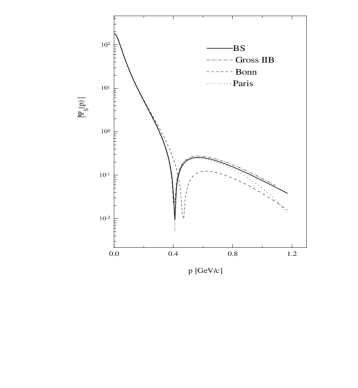
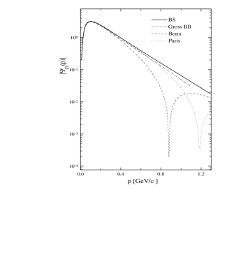
Figure 1: Comparison of the deuteron $S$ (left panel) and $D$-waves (right panel) obtained within different approaches: Bethe Salpeter umnikov (solid lines), Gross equation gross (dot-dahes lines), non relativistic Schrödinger approach with Bonn (dashed lines) and Paris (dotted lines) potentials.

With this solution we have analyzed different reactions with the deuteron in electromagnetic umnikov ; fsiHe3 ; yscaling , weak solar and hadronic processes dp ; our_chex ; our_brkp with the result that calculations within the BS formalism provide a much better agreement with experimental data in comparison with non relativistic approaches.

II.3 Covariant representation

It should be noted that the non relativistic Schrödinger approach belongs to the so-called ”instant-form” of dynamics diracForms , i.e. the solution of the Schrödinger equation is obtained in the center of mass system of the two-body system; being invariant only relative to the Lorentz transformation which leave the plane $t=const$ unchanged, it can not be boosted to another system of reference. This means that in non relativistic calculations the Lorentz boost effects in the wave function of a moving particle are always ignored. Probably this can be justified only at low momentum transfer (cf. e.g. Fig. 1). Contrarily, the BS amplitude, Eq. (1), is a covariant object by definition. Consequently, by applying the Lorentz transformation to the amplitude found in the rest system of the two-body system, one can obtain the BS solution in any system of reference. However, mathematically such a procedure is quite involved (see, e.g. Ref. static ), and in real calculations it becomes rather difficult to separate and investigate pure boost and other relativistic effects. In order to avoid such difficulties it is tempting to find a covariant representation of the amplitude, i.e., a representation within which the partial amplitudes are frame independent. Such a representation can be accomplished if one observes that, for instance in the deuteron case, one can form a new covariant basis of $4\times 4$ matrices from the available four independent matrix structures, $\hat{\xi}$, $(p\xi)\hat{I}$, $S(p_{1})^{-1}=\displaystyle\frac{\hat{P}}{2}+\hat{p}-m$, and $S(p_{2})^{-1}=\displaystyle\frac{\hat{P}}{2}-\hat{p}-m$, where $\xi$ is the deuteron polarization four-vector. Then the BS amplitude can be presented in the form

$$\Psi_{D}(P,p)=\left[{h_{1}}\hat{\xi}+{h_{2}}\frac{(p\xi)}{m}\right]+\frac{\hat{P}/2+\hat{p}-m}{m}\left[{h_{3}}\hat{\xi}+{h_{4}}\frac{(p\xi)}{m}\right]+$$

$$\left[{h_{5}}\hat{\xi}+{h_{6}}\frac{(p\xi)}{m}\right]\frac{\hat{P}/2-\hat{p}+m}{m}+\frac{\hat{P}/2+\hat{p}-m}{m}\left[{h_{7}}\hat{\xi}+{h_{8}}\frac{(p\xi)}{m}\right]\frac{\hat{P}/2-\hat{p}+m}{m},$$ (12)

where the ${h_{i}}$ are the sought covariant partial amplitudes. Obviously, these new amplitudes can be related to the non covariant ones by projecting (12) onto the corresponding basis. Explicit relations of covariant amplitudes ${h_{i}}$ in terms of spin-angular components can be found in Ref. static . Below we present an illustration of how the covariant amplitudes (12) can be used to analyze the process of backward elastic $pD$ scattering. This process has been investigated in the non relativistic Schrödinger approach within which the wave function in initial and final states has been taken for the deuteron at rest. The corresponding non relativistic helicity amplitudes and the cross section can be written as dp

$${\cal A}_{NR}\,=\,\left(u(P_{lab})+\frac{w(P_{lab})}{\sqrt{2}}\right)^{2}P_{lab}^{2},,\quad{\cal B}_{NR}\,=\,-\frac{3}{2}w(P_{lab})\,\left(2\sqrt{2}u(P_{lab})-w(P_{lab})\right)P_{lab}^{2},$$

$${\cal C}_{NR}\,=\,\left(u(P_{lab})+\frac{w(P_{lab})}{\sqrt{2}}\right)\left(u(P_{lab})-\sqrt{2}w(P_{lab})\right)P_{lab}^{2},,$$ (13)

$${\cal D}_{NR}\,=\,\frac{3w(P_{lab})}{\sqrt{2}}\left(u(P_{lab})+\frac{w(P_{lab})}{\sqrt{2}}\right)P_{lab}^{2},\quad\frac{d\sigma_{NR}}{d\Omega}\,=\,3\,\left(u^{2}(P_{lab})+w^{2}(P_{lab})\right)^{2}P_{lab}^{4},$$ (14)

where $P_{lab}$ is the momentum of the nucleon in the laboratory system, $u$ and $w$ are the two components of the deuteron wave function and the partial helicity amplitudes are defined as

$${\cal F}={\cal A}\,(\mbox{\boldmath{$\xi$}}_{M}\mbox{\boldmath{$\xi$}}^{+}_{M^{\prime}})+{\cal B}\,(\mbox{\boldmath{$n$}}\mbox{\boldmath{$\xi$}}_{M})(\mbox{\boldmath{$n$}}\mbox{\boldmath{$\xi$}}^{+}_{M^{\prime}})+i{\cal C}\,(\mbox{\boldmath{$\sigma$}}\cdot[\mbox{\boldmath{$\xi$}}_{M}\times\mbox{\boldmath{$\xi$}}^{+}_{M^{\prime}}])+i{\cal D}\,(\mbox{\boldmath{$\sigma$}}\mbox{\boldmath{$n$}})(\mbox{\boldmath{$n$}}\cdot[\mbox{\boldmath{$\xi$}}_{M}\times\mbox{\boldmath{$\xi$}}^{+}_{M^{\prime}}]).$$ (15)

In Eq. (15) $\mbox{\boldmath{$\xi$}}_{M}$ is the polarization 3-vector of the deuteron at rest, ${\cal F}$ is the total amplitude of the process. This amplitude can be found by calculating the corresponding one-nucleon-exchange Feynman diagram and using the covariant BS amplitudes (12) which allow to write explicitly the dependence on the polarization vector $\mbox{\boldmath{$\xi$}}_{M}$ and, consequently, to determine the partial amplitudes $\cal A,B,C$ and $\cal D$. The result of a calculation, with preserving only the main $"++"$ components, is dp

$$\frac{d\sigma_{0}}{d\Omega} = 3\,\left(\Psi_{S}^{2}(P_{lab})+\Psi^{2}_{D}(P_{lab})\right)^{2}\,P_{lab}^{4}\left(1+\frac{P_{lab}^{2}}{2m^{2}}+\frac{29P_{lab}^{4}}{16m^{4}}+\frac{83P_{lab}^{6}}{32m^{6}}+\cdots\right),$$ (16)

$${\cal A}_{0} = P_{lab}^{2}\,\left(\Psi_{S}(P_{lab})-\frac{\Psi_{D}(P_{lab})}{\sqrt{2}}\right)^{2}\,{\cal L}(P_{lab}),$$ (17)

$${\cal B}_{0} = P_{lab}^{2}\ \frac{3}{2}\Psi_{D}(P_{lab})\,\left(2\sqrt{2}\Psi_{S}(P_{lab})+\Psi_{D}(P_{lab})\right)\,{\cal L}(P_{lab}),$$ (18)

$${\cal C}_{0}\, = P_{lab}^{2}\,\left(\Psi_{S}(P_{lab})-\frac{\Psi_{D}(P_{lab})}{\sqrt{2}}\right)\left(\Psi_{S}(P_{lab})+\sqrt{2}\Psi_{D}(P_{lab})\right)\,{\cal L}(P_{lab}),$$ (19)

$${\cal D}_{0} = -\,P_{lab}^{2}\,\frac{3}{\sqrt{2}}\Psi_{D}(P_{lab})\left(\Psi_{S}(P_{lab})-\frac{\Psi_{D}(P_{lab})}{\sqrt{2}}\right)\,{\cal L}(P_{lab}),$$ (20)

where $\Psi_{S,D}$ are the main, $"++"$, components of the deuteron (see Fig. 1), and ${\cal L}(P_{lab})=\left(1+\frac{P_{lab}^{2}}{4m^{2}}+\frac{7P_{lab}^{4}}{8m^{4}}+\cdots\right)$. It can be seen that the analytical expressions for relativistic and non relativistic helicity amplitudes are rather similar, except for the factor ${\cal L}(P_{lab})$ which depends on the velocity of the deuteron and obviously describes the Lorentz boost effects. Other pure relativistic corrections appear in the cross section from the contribution of the negative $P$-waves dp . In Fig. 2, we exhibit results of calculations of the differential cross section with emphasis on different contributions. The notation in Fig. 2 is quite self-explanatory. One can conclude that at large values of the initial energy the relativistic effects increase and become significant at $P_{lab}\geq 0.35-0.4\ GeV/c$.

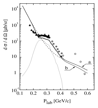
Figure 2: The spin averaged cross section $d\sigma/d\Omega$ for the backward elastic $dp$ scattering in the center of mass as a function of the momentum of the detected proton in the laboratory system. Left panel: Dashed line - contribution of the positive BS waves; long-dashed line - Lorentz boost effects, solid line - full BS calculations; dotted line-results of the non relativistic approach with the Bonn potential wave function. Experimental data are from exppD . Right panel: dashed line - contribution of the one-nucleon exchange mechanism only; dotted line - contribution of the triangle diagram ($\Delta$-isobars); solid lines - the full BS calculations with $P$ waves (a) and without $P$ waves (b).

II.4 The one-iteration approximation

As mentioned above, the basis of Dirac matrices turns out to be the most appropriate representation in solving numerically the BS equation. Transitions to other bases can be accomplished by performing the corresponding unitary transformations. In such a way one can obtain numerical solutions of the BS equation in representations, which are most relevant for the considered problem and one can investigate numerically different aspects of the process. However besides numerical investigations, it is useful to have a mathematical method for analytical estimates of the considered effects. Remind, that often in non relativistic approaches one takes into account relativistic corrections by calculating additional diagrams with meson exchange currents, nucleon-antinucleon pair currents etc. It is intuitively clear that some of these corrections must be included already in the relativistic amplitude via negative $P$ waves and Lorentz boost effects which are absent in the non relativistic calculations. An estimate of the role of $P$ waves can be accomplished by solving the BS equation in the so-called one-iteration approximation (OIA). The spirit of the method follows from the observation that if, when solving numerically the BS equation by iterations, the trial function is close to the exact solution, the latter one can be obtained by performing only one or two iterations.

As illustrated in Fig. 1, at low values of the relative momentum $p$ the exact solution coincides, to a good accuracy, with the non relativistic solution of the Schroedinger equation. This is a hint that, using the non relativistic deuteron wave function as trial function, the number of iterations in solving the BS equation can be strongly reduced. Moreover, at low and intermediate values of $p$ the first iteration with the non relativistic solution as trial function can serve as a good approximation of the exact solution.

As an example, let us consider the BS equation for the deuteron partial vertices in the spin-angular harmonics basis (11):

$$G_{\alpha}(k_{0},|{\mbox{\boldmath$k$}}|)=-\sum_{b}g_{b}^{2}\int\frac{{\mbox{\boldmath$p$}}^{2}d|{\mbox{\boldmath$p$}}|\,dp_{0}}{4\pi^{2}}W_{\alpha\beta}(k,p)\,\Psi_{\beta}(p_{0},|{\mbox{\boldmath$p$}}|),$$ (21)

$$W_{\alpha\beta}(k,p)\equiv\sum_{lm}\frac{Q_{l}(z)}{2\pi|{\mbox{\boldmath$p$}}||{\mbox{\boldmath$k$}}|}\int\!d\Omega_{k}\,d\Omega_{p}\,Y_{lm}({\mbox{\boldmath$p$}})\,Y^{*}_{lm}({\mbox{\boldmath$k$}})\,\mbox{Tr}\!\left[\Gamma_{\alpha}^{+}(-{\mbox{\boldmath$k$}})\gamma_{b}\Gamma_{\beta}({\mbox{\boldmath$p$}})\gamma_{b}\right].$$

The OIA method implies: i) in (21) all ”negative” waves are put equal to zero, ii) the $k_{0}$ and $p_{0}$ dependencies in the partial kernels $W_{\alpha\beta}(k,p)$ and in vertices $G_{{}^{3}S_{1}^{++}}$ and $G_{{}^{3}D_{1}^{++}}$ are disregard, i.e. $W_{\alpha\beta}(k,p)\simeq W_{\alpha\beta}(|{\mbox{\boldmath$k$}}|,|{\mbox{\boldmath$p$}}|),$ $G_{++}(p_{0},|{\bf p}|)\simeq G_{++}(0,|{\bf p}|)$, iii) the trial function is taken as solution of the non relativistic Schroedinger equation for the deuteron, and iv) the negative (P) waves are obtained only by one iteration in Eq. (21). For instance, for the pseudo-scalar isovector exchange we get

$$W_{P_{3}^{-+}\to S^{++}}=-W_{P_{3}^{+-}\to S^{++}}=\sqrt{2}W_{P_{1}^{+-}\to S^{++}}=\sqrt{2}W_{P_{1}^{-+}\to S^{++}}={\cal N}\sqrt{2}\left[Q_{0}(y)|\vec{k}|-Q_{1}(y)|\vec{p}|\right],$$ (22)

$$W_{P_{3}^{+-}\to D^{++}}=-W_{P_{3}^{-+}\to D^{++}}=\sqrt{2}W_{P_{1}^{+-}\to D^{++}}=\sqrt{2}W_{P_{1}^{-+}\to D^{++}}={\cal N}\left[-Q_{1}(y)|\vec{p}|+Q_{2}(y)|\vec{k}|\right],$$ (23)

where ${\cal N}=-\sqrt{3}/(2|\vec{p}||\vec{k}|E_{k})$, $E_{k}=\sqrt{{\bf k}^{2}+m^{2}}\sim m$, $m$ being the nucleon mass. In coordinate space one has

$$\int\frac{p^{2}dp}{2|\vec{p}||\vec{k}|}\left[|\vec{k}|Q_{0}(z)-|\vec{p}|Q_{1}(z)\right]\Psi_{S}(|\vec{p}|)=\int\,dr\frac{\Psi_{S}(r)}{r}{\rm e}^{-\mu r}(1+\mu r)j_{1}(kr),$$ (24)

$$\int\frac{p^{2}dp}{2|\vec{p}||\vec{k}|}\left[|\vec{p}|Q_{1}(z)-|\vec{k}|Q_{2}(z)\right]\Psi_{D}(|\vec{p}|)=-\int\,dr\frac{\Psi_{D}(r)}{r}{\rm e}^{-\mu r}(1+\mu r)j_{1}(kr),$$ (25)

where $\mu$ stands for the pion mass. Then the result for the negative $P$-waves for the pseudo-scalar one-boson exchange reads

$$\Psi_{P^{+-}_{3}(P^{+-}_{1})}(P_{lab})=-g_{\pi}^{2}\frac{2\sqrt{3}}{M_{d}E_{p}^{\prime}}\int\limits_{0}^{\infty}dr\,\frac{{\rm e}^{-\mu r}}{r}\,(1+\mu r)\,{\rm j_{1}}(rP_{lab})\left[N_{u}\,u(r)+N_{w}\,w(r)\right],$$ (26)

where $u(r)$ and $w(r)$ are the non-relativistic deuteron wave functions in the coordinate representation, and $g_{\pi}^{2}\approx$ 14.5 is the pion-nucleon coupling constant. The normalization factors are $N_{u}=\sqrt{2}$ (1) and $N_{w}=$ -1 ($\sqrt{2}$) for $P^{+-}_{3}$ $(P^{+-}_{1})$ waves. With this negative-energy waves one may estimate the origin of the relativistic corrections computed within the non-relativistic limit as additional contribution to the impulse approximation diagrams, such as meson exchange currents and $N\bar{N}$ pair production currents. As an example we present here the relativistic corrections to the partial amplitude $\cal A$ (15)

$$\delta{\cal A} = -g_{\pi}^{2}P_{lab}^{3}\frac{192\sqrt{2}\pi}{M_{d}E_{p}^{\prime}}\int\limits_{0}^{\infty}dr\,\frac{{\rm e}^{-\mu r}}{r}\,(1+\mu r)\,{\rm j_{1}}(rP_{lab})\left[\sqrt{2}\,u(r)-\,w(r)\right]\left(\Psi_{S}-\frac{1}{\sqrt{2}}\Psi_{D}\right)$$ (27)

which is similar to the expressions obtained in non-relativistic evaluations of the so-called “catastrophic” and pair production diagrams in electro-disintegration processes of the deuteron disintegration and also similar to the results of a computation of the triangle diagrams usually considered in the elastic $pD$ processes dp ; wilkin ; nakamura . Another example concerns the calculation of the effects of final state interaction in reactions of deuteron break-up with two nucleons in the final state with low relative energy exper . Exact calculations require also the solution of the BS equation for the scattering state in the continuum. At the considered energies one can avoid the involved procedure of solving the BS equation in the continuum by employing the OIA in the same manner as described above. In Fig. 3 we present results of calculations of the cross section for the reaction $pD\to(pp)n$ within the OIA for the BS amplitudes and a comparison with non relativistic results and available experimental data. It can be seen that relativistic calculations provide a much better agreement with data.

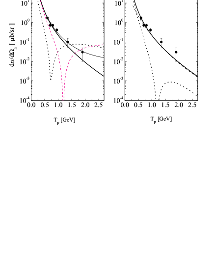
Figure 3: The cross section for the reaction $pD\to(pp)n$. Left panel: dotted and dashed lines represent the calculations within the nonrelativistic and relativistic impulse approximation, respectively; the two solid lines are the results which include the final state interaction in the (pp) - pair in a ${}^{1}S_{0}$ state calculated within the one-iteration approximation. The lower and upper solid lines have been obtained with and without cut-off form factors in the BS equation. Right panel: the relative contribution of the deuteron relativistic $S$ (dotted line) and $D$ (dashed line) components to the total cross section. Experimental data are from exper

.

III Exhausting method

Notice that the above mentioned methods are higly suitable for solving the BS equation by iterations, which provide the solution of ground state of the system. This is quite acceptable in most calculations for the deuteron and light mesons. However, heavier mesons (e.g. $J/\Psi$, $D$ mesons) possess an entire mass spectrums with various, experimentally known, transitions to the ground state. Consequently, one needs a generalization of the iteration procedure which would allow to find the energy spectrum of the excited states and the corresponding amplitudes. The ”exhausting” (depletion) method nashYaph is the one within which the ground and excited states of the system can be found by solving the BS equation by iteration. The main idea of the method can be illustrated in the case of the scalar BS equation with scalar interaction. The corresponding equation reads

$$\varphi_{JM}(p)=i\,g^{2}\,S(p_{1})S(p_{2})\int\!\frac{d^{4}p^{\prime}}{(2\pi)^{4}}~{}\frac{1}{(p-p^{\prime})^{2}-\mu^{2}+i\varepsilon}~{}\varphi_{JM}(p^{\prime}),$$ (28)

where the scalar propagator is $S(p)=1/(p^{2}-m^{2}+i\varepsilon)$ and $JM$ are the total angular momentum and its projection. It is more convenient the introduce the BS equation for the vertex function, $\varphi_{JM}(p)=S(p_{1})~{}{\cal G}_{JM}(p)~{}S(p_{2})$. Then in Euclidian space one has

$${\cal G}_{JM}(p)=\lambda~{}\int d^{4}p^{\prime}~{}\underbrace{\frac{1}{(2\pi)^{4}}~{}\frac{1}{[(E^{2}_{{\mbox{\boldmath$p$}}}+p_{0}^{2}-\frac{1}{4}M_{B}^{2})^{2}+p_{0}^{2}M_{B}^{2}][(p-p^{\prime})^{2}+\mu^{2}]}}_{K(p,p^{\prime};M_{B})}~{}{\cal G}_{JM}(p^{\prime}),$$ (29)

where $\lambda\equiv g^{2}$. Obviously, at fixed $M_{B}$ Eq. (29) is a Fredholm type eigenvalue equation relative to $\lambda_{iJ}=g^{2}_{iJ}$ with eigenfunctions ${\cal G}_{JM}^{i}(p)$. The set of eigenvalues $\lambda_{iJ}\equiv\lambda_{iJ}(M_{B})$ is also called the spectrum of (29) relative to the coupling constant. It is straightforward to establish a correspondence between the mass spectrum of the equation and its spectrum on coupling constant; it is sufficient to find the spectrum $\lambda_{iJ}(M_{B})$ at all allowed values of $M_{B},~{}0\leq M_{B}\leq 2m$ and to inverse the problem, i.e. to fix $\lambda$ at its actual value and to find the corresponding value of $M_{B}$. In such a way, each $\lambda_{i}$ receives its particular value of $M_{B}$, which forms the mass spectrum of the equation. From the rigorous Hilbert-Schmidt theory of symmetric integral equations it is known that: i) the spectrum of Eq. (29) is discrete and real with a nondecreasing sequence of $\lambda_{iJ}$ $|\lambda_{1}|\leq|\lambda_{2}|\leq...\leq|\lambda_{n}|\ldots$, ii) the corresponding eigenfunctions ${\cal G}^{i}_{JM}(p)$ and the corresponding amplitudes $\varphi^{i}_{JM}(p)$ form a bi-orthogonal basis $\int d^{4}p~{}\varphi^{i*}_{JM}(p)~{}{\cal G}^{j}_{J^{\prime}M^{\prime}}(p)=\delta_{ij}\delta_{JJ^{\prime}}\delta_{MM^{\prime}}$ within which the kernel $K(p,p^{\prime};M_{B})$ can be represented as

$$K(p,p^{\prime};M_{B})=\sum\limits_{i=1}^{\infty}\sum\limits_{JM}\frac{1}{\lambda_{iJ}}~{}{\cal G}^{i}_{JM}(p)~{}\varphi^{i*}_{JM}(p^{\prime}).$$ (30)

For the scalar equation the partial amplitudes have a particularly simple form, ${\cal G}^{i}_{JM}(p)=\frac{1}{|{{\mbox{\boldmath$p$}}}|}G^{i}_{J}(\tilde{p}){\mbox{\large{Y}}}_{JM}(\Omega_{p}),$ where for brevity the notation $\tilde{p}=(p_{0},~{}|{{\mbox{\boldmath$p$}}}|)$ has been introduced. Then the partial vertices $G^{i}_{J}(\tilde{p})$ read

$$G^{i}_{J}(\tilde{p})=\lambda_{iJ}~{}\int d\tilde{p}^{\prime}~{}K^{J}(\tilde{p};\tilde{p}^{\prime};M_{B})~{}G^{i}_{J}(\tilde{p}^{\prime}),$$ (31)

$$K^{J}(\tilde{p};\tilde{p}^{\prime};M_{B})=\frac{1}{(2\pi)^{3}}~{}\frac{1}{[(E^{2}_{{\mbox{\boldmath$p$}}}+p_{0}^{2}-\frac{1}{4}M_{B}^{2})^{2}+p_{0}^{2}M_{B}^{2}]}~{}Q_{J}({y}).$$ (32)

Notice that the partial vertices $G^{i}_{J}(\tilde{p})$ together with the partial amplitudes $\varphi_{J}^{i}$ also form a bi-orthogonal basis, hence the partial kernels $K^{J}(\tilde{p};\tilde{p}^{\prime};M_{B})$ can also be written in the form

$$K^{J}(\tilde{p};\tilde{p}^{\prime};M_{B})=\sum\limits_{i=1}^{\infty}\frac{1}{\lambda_{iJ}}~{}G^{i}_{J}(\tilde{p})~{}\varphi^{i}_{J}(\tilde{p}^{\prime}).$$ (33)

Now we are in the position to formulate the exhausting method for the Eq. (29). Consider the problem of finding the lowest eigenvalue $\lambda_{1J}$ at fixed $J$ and $M_{B}$. Schematically, Eq. (31) read

$$\frac{1}{\lambda_{1J}}~{}G^{i}_{J}=K^{J}~{}G^{i}_{J}.$$ (34)

Let now choose a trial function $\chi(\tilde{p})$ and form a sequence of functions $K^{J}~{}\chi$, $(K^{J})^{2}\chi$, …, $(K^{J})^{n}\chi$. The trial function $\chi$ can be decomposed on the complete set of functions $G^{i}_{J}$, $\chi=\sum\limits_{i=1}^{\infty}c_{i}~{}G^{i}_{J},$ where $c_{i}=\int d\tilde{p}~{}\varphi^{i}_{J}(\tilde{p})~{}\chi(\tilde{p})$ and from Eq. (34) one gets

$$K^{J}~{}\chi=\sum\limits_{i=1}^{\infty}c_{i}~{}\frac{1}{\lambda_{iJ}}~{}G^{i}_{J},\quad(K^{J})^{2}\chi=\sum\limits_{i=1}^{\infty}c_{i}~{}\frac{1}{\lambda_{1J}^{2}}~{}G^{i}_{J},\ldots,\quad(K^{J})^{n}\chi=\sum\limits_{i=1}^{\infty}c_{i}~{}\frac{1}{\lambda_{1J}^{n}}~{}G^{i}_{J}.$$ (35)

At each $n$-th iteration one considers the ratio $(K^{J})^{n}\chi/(K^{J})^{n-1}\chi$, which at large enough $n$ provides the lowest eigenvalue of the spectrum:

$$\frac{(K^{J})^{n}\chi}{(K^{J})^{n-1}\chi}=\frac{\sum\limits_{i=1}^{\infty}c_{i}~{}\frac{1}{\lambda_{iJ}^{n}}~{}G^{i}_{J}}{\sum\limits_{i=1}^{\infty}c_{i}~{}\frac{1}{\lambda_{iJ}^{n-1}}~{}G^{i}_{J}}=\frac{1}{\lambda_{1J}}~{}\frac{c_{1}~{}G^{1}_{J}+\sum\limits_{i=2}^{\infty}c_{i}~{}\left(\frac{\lambda_{1J}}{\lambda_{iJ}}\right)^{n}~{}G^{i}_{J}}{c_{1}~{}G^{1}_{J}+\sum\limits_{i=2}^{\infty}c_{i}~{}\left(\frac{\lambda_{1J}}{\lambda_{iJ}}\right)^{n-1}~{}G^{i}_{J}}\stackrel{{\scriptstyle n\to\infty}}{{\Longrightarrow}}\frac{1}{\lambda_{1J}}.$$ (36)

Figure 4: The coupling constant $g$ vs. the value of the mass $M_{B}$ of the bound system for two values of the total angular momentum $J=0,2$. The solid curves correspond to the ground state, while the dashed lines are for the first excited state. Intersections of the horizontal line $g=10$ with the respective curve determine the energy spectrum of the system: $M_{B}\simeq 1.75\ GeV$, $M_{B}\simeq 1.94\ GeV$ for $J=0$ and $M_{B}\simeq 1.97\ GeV$, $M_{B}\simeq 1.98\ GeV$ for $J=2$.

Equations (35) and (36) demonstrate how one finds the ground state solution, i.e. the eigenvalue $\lambda_{1J}$ and the eigenfunction $G_{1J}$ can be found. Now, to find the next excited eigenvalue $\lambda_{2J}$, one defines a new kernel $K^{J,1}$ for which the new BS equation has the same spectrum $\lambda_{iJ}$ and eigenfunctions $G_{iJ}$ ($i=2...n$) except the first state $i=1$. For such a kernel, $\lambda_{2J}$ and $G_{2J}$ would serve as ground state solution. The new kernel which obeys these conditions is

$$K^{J,1}(\tilde{p},\tilde{p}^{\prime};M_{B})=K^{J}(\tilde{p},\tilde{p}^{\prime};M_{B})-\frac{1}{\lambda_{1J}}~{}G^{1}_{J}(\tilde{p})~{}\varphi^{1}_{J}(\tilde{p}^{\prime})=\sum\limits_{i=2}^{\infty}\frac{1}{\lambda_{iJ}}~{}G^{i}_{J}(\tilde{p})~{}\varphi^{i}_{J}(\tilde{p}^{\prime}).$$ (37)

It can be seen that all eigenfunctions $G^{i}_{J}$ of the kernel $K^{J}$, except $G^{1}_{J}$, are the eigenfunctions of the new kernel $K^{J,1}$ with the same eigenvalue spectrum $\lambda_{iJ}$. Obviously, the lowest eigenvalue of $K^{J,1}$ is $\lambda_{2J}$, which can be found by the same iteration procedure, i.e. via Eqs. (35) and (36). Analogously one finds the next solutions $i=3,4\ldots$ from the recurrent kernel

$$K^{J,n}(\tilde{p},\tilde{p}^{\prime};M_{B})=K^{J,n-1}(\tilde{p},\tilde{p}^{\prime};M_{B})-\frac{1}{\lambda_{nJ}}~{}G^{n}_{J}(\tilde{p})~{}\varphi^{n}_{J}(\tilde{p}^{\prime})=\sum\limits_{i=n+1}^{\infty}\frac{1}{\lambda_{iJ}}~{}G^{i}_{J}(\tilde{p})~{}\varphi^{i}_{J}(\tilde{p}^{\prime}).$$ (38)

As an example of application of the method, results of calculations of the eigenvalues $g=\frac{1}{\lambda}$ as functions of the binding mass $M_{B}$ are presented in Fig. 4 for first two ground states of a system of two equal masses particles with total angular momentum $J=0$ and $J=2$ (solid lines) and two excited states (dashed lines), respectively. It is clear that, if the coupling constant is known from independent experiments, the mass spectrum of the system can be easily recovered (see illustration in Fig. 4 for $g=10$).

A generalization of the method for the spinor-spinor BS equation can be found in nashYaph .

IV Hyperspherical harmonics

The considered methods are convenient for solving numerically the BS equation by an iteration procedure. The obtained solution presents a set of two-dimensional arrays of the partial amplitudes $\psi_{i}$, cf. Eq. (4). In practice, such a representation of the solution can cause difficulties in specific calculations which require two-dimensional interpolations of such arrays, e.g. in attempts to determine analytical parametrizations of the numerical solution, in performing the inverse Wick rotation, etc. This is particularly awkward to use such solutions if one solves the BS equation for $q\bar{q}$ bound systems (mesons) in nonperturbative QCD. In the later case, the BS equation must be solved simultaneously with the Dyson-Schwinger equation to generate dynamically the masses of the constituent quarks. Numerical solutions in form of one-dimensional arrays would be much more appropriate for tthese problems. This can be achieved by decomposing the partial amplitudes over the three-dimensional hyperspherical harmonics basis in Euclidian space

$$Z_{nlm}(\chi,\theta,\phi)=X_{nl}(\chi)Y_{lm}(\theta,\phi);\quad X_{nl}(\chi)=\sqrt{\frac{2^{2l+1}}{\pi}\frac{(n+1)(n-l)!l!^{2}}{(n+l+1)!}}\sin^{l}\chi C_{n-l}^{l+1}(\cos\chi),$$ (39)

where $C_{n-l}^{l+1}$ are the usual Gegenbauer polynomials, $\cos\chi=\displaystyle\frac{p_{0}}{\hat{p}};\,\,\sin\chi=\displaystyle\frac{|{\bf p}|}{\hat{p}};\,\,\hat{p}=\sqrt{p_{0}^{2}+{\bf p}^{2}}$. The BS vertices (amplitudes) are decomposed over the complete set of spin-angular harmonics.

$${\cal G}(p_{0},{\mbox{\boldmath$p$}}) = \sum\limits_{\alpha}g_{\alpha}(p_{0},|{\mbox{\boldmath$p$}}|)\,\Gamma_{\alpha}({\mbox{\boldmath$p$}})$$ (40)

with the coefficients $g_{\alpha}(p_{0},|{\mbox{\boldmath$p$}}|)$ as

$$g_{\alpha}(p_{0},{\mbox{\boldmath$p$}})=\sum_{j,n,m}^{\infty}g^{j}_{\alpha}(\hat{p})\ Z_{jlm}(\chi_{p},\theta_{p},\phi_{p}).$$ (41)

Note that, in order to be able to carry out the $\chi_{p},\theta_{p},\phi_{p}$ - integrations analytically, the spin-orbital basis must be slightly redefined (see Ref. fbBayer for details). The scalar part of the interaction kernel is also represented in terms of hyperspherical harmonics

$$\frac{1}{(p-k)^{2}+\mu^{2}} = 2\pi^{2}\sum_{nlm}\frac{1}{n+1}V_{n}(\hat{p},\hat{k})Z_{nlm}(\chi_{p},\theta_{p},\phi_{p})Z_{nlm}^{*}(\chi_{k},\theta_{k},\phi_{k}),$$

$$V_{n}(\hat{p},\hat{k}) = \frac{4}{(\Lambda_{+}+\Lambda_{-})^{2}}\left(\frac{\Lambda_{+}-\Lambda_{-}}{\Lambda_{+}+\Lambda_{-}}\right)^{n};\quad\Lambda_{\pm}=\sqrt{(\hat{p}\pm\hat{k})^{2}+\mu^{2}}.$$ (42)

By inserting Eqs. (40)-(42) into the BS equation one obtains a system of one-dimensional integral equations for the partial amplitudes

$$g_{1}(p_{0},|{\mbox{\boldmath$p$}}|)=\sum_{j=1}^{\infty}g_{1}^{j}(\hat{p})\,X_{2j-2,0}(\chi_{p});\quad g_{2}(p_{0},|{\mbox{\boldmath$p$}}|)=\sum_{j=1}^{\infty}g_{2}^{j}(\hat{p})\,X_{2j-2,0}(\chi_{p});$$ (43)

$$g_{3}(p_{0},|{\mbox{\boldmath$p$}}|)=\sum_{j=1}^{\infty}g_{3}^{j}(\hat{p})\,X_{2j-1,1}(\chi_{p});\quad g_{4}(p_{0},|{\mbox{\boldmath$p$}}|)=\sum_{j=1}^{\infty}g_{4}^{j}(\hat{p})\,X_{2j,1}(\chi_{p}),$$ (44)

where

$$g^{j}_{1,2}(\hat{p}) = -g^{2}\ b_{1,2}\int\limits_{0}^{\infty}\frac{d\hat{k}\,{\hat{k}}^{3}}{8\pi^{2}(2j-1)}\,V_{2j-2}(\hat{p},\hat{k})\sum\limits_{n=1}^{4}\sum\limits_{m=1}^{\infty}A^{1,2\ n}_{jm}(\hat{k})\,g_{n}^{m}(\hat{k}),$$ (45)

$$g^{j}_{3}(\hat{p}) = -g^{2}b_{3}\int\limits_{0}^{\infty}\frac{d\hat{k}\,{\hat{k}}^{3}}{8\pi^{2}\,2j}\,V_{2j-1}(\hat{p},\hat{k})\sum\limits_{n=1}^{4}\sum\limits_{m=1}^{\infty}A^{3\ n}_{jm}(\hat{k})\,g_{n}^{m}(\hat{k}),$$ (46)

$$g^{j}_{4}(\hat{p}) = -g^{2}b_{4}\int\limits_{0}^{\infty}\frac{d\hat{k}\,{\hat{k}}^{3}}{8\pi^{2}(2j+1)}\,V_{2j}(\hat{p},\hat{k})\sum\limits_{n=1}^{4}\sum\limits_{m=1}^{\infty}A^{4\ n}_{jm}(\hat{k})\,g_{n}^{m}(\hat{k}).,$$ (47)

where $b_{i}$ and $A^{\alpha\ n}_{jm}$ are known coefficients, whose explicit expressions can be found in Ref. fbBayer . It can be seen from Eqs. (45)-(47) that the partial amplitudes within the hyperspherical basis are functions of only one variable. Instead, the obtained system of integral equations is infinite. At first glance, this may cause unresolvable problems. However, in practice, when solving the system (45)-(45) a good convergence can be achieved by considering only the few first terms in (43) and (44), usually up to $j=3-4$ fbBayer . In Fig. 5 we present an example of the use of hyperspherical basis in solving the BS equation for the ${}^{1}S_{0}$ channel. The obtained solution can be fitted by a simple formula

$$g_{1}^{j}(\hat{p})\simeq\left[\frac{\hat{p}^{2}}{\hat{p}^{2}+b_{j}^{2}}\right]^{j-1}\sum\limits_{l=1}^{4}\frac{a_{jl}\,\hat{p}^{2l-2}}{(\hat{p}^{2}+b_{j}^{2})^{l}}$$ (48)

which is extremely useful in further analyses of the solution in Minkowski space. The fitted parameters $a_{j}$ and $b_{j}$ can be found in Ref. fbBayer .

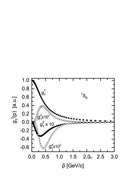
Figure 5: Functions $g_{1}^{j},j=1,\ldots,4$, eq. (43)-(44). Full squares correspond to $g_{1}^{1}$; full circles to $g_{1}^{2}$ multiplied by 10; triangles to $g_{1}^{3}$ multiplied by 100; open circles to $g_{1}^{4}$ multiplied by 1000; the solid lines correspond to the fitted functions $g_{1}^{j}$ by formula (48). The overall normalization constant is arbitrary.

V Summary

In this mini-review we briefly considered different methods to solve the BS equation in Euclidian space. It is shown that the complete set of Dirac matrices is the most convenient way to decompose the BS amplitude and to find the partial amplitudes by iteration procedure. The transition to other representation, e.g. to the spin-angular harmonics basis or to the covariant representation can be accomplished by performing the corresponding unitary transformation. Examples of numerical solution for the deuteron and applications for the calculation of matrix elements of observables are presented, which illustrate the role of relativistic corrections and Lorentz boost effects.

A generalization of the iteration method to find the energy spectrum of the BS equation is also discussed. It is shown that the Hilbert-Schmidt bi-orthogonal basis can define a mathematical method, known as the ”exhausting method”, to find numerically the energy spectrum and the corresponding partial amplitudes for the excited states of two-body systems.

The hyperspherical harmonics basis is shown to be the most appropriate one in finding the BS solution in form of one-dimensional numerical arrays. This is extremely convenient in analytical continuation of the solution back to Minkowski space and in solving simultaneously the Dyson-Schwinger and BS equation for the $q\bar{q}$ bound states (mesons) in nonperturbative QCD.

References

- (1) Rupp, G., Tjon, J.A.: Phys. Rev. C45, 2133 (1992)
- (2) Fleischer, J., Tjon, J.A.: Nucl. Phys. B84, 375 (1975)
- (3) Zuilhof, M.J., Tjon, J.A.: Phys. Rev. C22, 2369 (1980) and references therein
- (4) Umnikov, A.Yu., Kaptari, L.P., Khanna, F.C.: Phys. Rev. C56, 1700 (1997)
- (5) Holl, A., Krassnigg, A., Maris, P., Roberts, C.D., Wright, S.V.: Phys. Rev. C71, 065204 (2005)
- (6) Gross, F., Van Orden, J.W., Holinde, K.: Phys. Rev. C45, 2094 (1992)
- (7) Puzynin, I.V., et al.: Phys. Part. Nucl. 30, 87 (1999)
-
(8)
Mangin-Brinet, M., Carbonell, J., Karmanov, V.A.:
Phys. Rev. C68, 055203 (2003);
Mangin-Brinet, M., Carbonell, J., Karmanov, V.A.: Phys. Rev. D64, 125005 (2001). - (9) Frederico, T., Sales, J.H.O., Carlson, B.V., Sauer, P.U.: Few Body Syst. 33, 89 (2003)
- (10) Efimov, G.V.: Few-Body Syst. 33, 199 (2003)
- (11) Bakker, B.L.G., van Iersel, M., Pijlman, F.: Few Body Syst. 33, 27 (2003)
- (12) Carbonell, J., Desplanques, B., Karmanov, V.A. Mathiot, J.-F.: Phys. Rept. 300, 215 (1998)
- (13) Nieuwenhuis, T., Tjon, J.A.: Few-Body Syst. 21 167 (1996)
-
(14)
Lev, F.M., Pace, E., Salme, G.: Phys. Rev. C62, 064004 (2000)
Lev, F.M., Pace, E., Salme, G.: Phys. Rev. Lett. 83, 5250 (1999)
de Melo, J.P.B.C., Frederico, T., Pace, E., Salme, G.: Phys. Lett. B581, 75 (2004) - (15) Salpeter, E.E., Bethe, H.A.: Phys. Rev. 84, 1232 (1951)
- (16) Wick, G.C.: Phys. Rev. 96, 1124 (1954).
- (17) Mandelstam S.: Proc. Roy. Soc. (London) A233, 248 (1955)
- (18) Nakanishi, N.: Prog. Theor. Phys. Suppl. 43, 1 (1969)
- (19) Kaptari, L.P., Umnikov, A.Yu., Bondarenko, S.G., Kazakov, K.Yu., Khanna, F.C., Kämpfer, B.: Phys. Rev. C54, 986 (1996)
-
(20)
Ciofi degli Atti C., Kaptari L.P.: Phys. Rev. C71, 024005 (2005);
Ciofi degli Atti C., Kaptari L.P., Treleani D.: Phys. Rev. C63, 044601 (2001) - (21) Kubis J.J.: Phys. Rev. 6, 547 (1972)
- (22) Ciofi degli Atti C., Faralli D, Kaptari L.P., Umnikov A.Yu.: Phys. Rev. C60, 034003 (1999)
- (23) Kaptari L.P., Kämpfer B., Grosse E.: J. Phys. G26 (2000) 1423
- (24) Kaptari L.P., Kämpfer B., Dorkin S.M., Semikh S.S.,: Phys. Rev. C57, 1097 (1998)
- (25) Kaptari L.P., Kämpfer B., Semikh S.S., Dorkin S.M.: Eur. Phys. J. A17, 119 (2003); ibid J. Phys. G30, 1115 (2004)
-
(26)
Kaptari L.P., Kämpfer B., Semikh S.S., Dorkin S.M.,:
Eur. Phys. J. A19, 301 (2004);
Semikh, S.S., Dorkin, S.M., Beyer, M., Kaptari, L.P.: Phys. Atom. Nucl. 68, 2022 (2005) - (27) Dirac P.A.M.: Rev. Mod. Phys.bf 21, 392 (1949)
-
(28)
Nakamura A.,Satta L.: Nucl. Phys. A445, 706 (1985)
and references therein;
Berthet P. et al.: Journal of Phys. G8, L111 (1982);
Bonner B.E. et al.:, Phys. Rev. Lett. 39, 1253 (1977) ;
Dubal L. et al.: Phys. Rev. D9, 597 (1974) - (29) Bondarenko, S.G., Burov, V.V., Beyer, M., Dorkin, S.M.: Phys. Rev. C58, 3143 (1998)
- (30) Craigie N.S., Wilkin C.: Nucl. Phys. B14, 477 (1969)
- (31) Nakamura A., Satta L.: Nucl. Phys. A 445, 706 (1985)
- (32) Komarov V.I. et al.: Phys. Lett., B553, 179 (2003).
- (33) Dorkin S.M., Kaptari L.P., Semikh S.S.: Phys. Atom. Nucl. bf 60, 1629 (1997).
- (34) Dorkin S.M., Beyer M., Semikh S.S., Kaptari L.P.: Few Body Syst. 42, 1 (2008)