The Direct Monodromy Problem of Painleve-I

Abstract

The Painleve first equation can be represented as the equation of isomonodromic deformation of a Schrödinger equation with a cubic potential. We introduce a new algorithm for computing the direct monodromy problem for this Schrödinger equation. The algorithm is based on the geometric theory of Schrödinger equation due to Nevanlinna

1 Introduction

Painlevé equations form the core of what may be called "modern special function theory". Indeed, since the 1970s’ pioneering works of Ablowitz and Segur, and McCoy, Tracy and Wu the Painlevé functions have been playing the same role in nonlinear mathematical physics that the classical special functions, such as Airy functions, Bessel functions, etc., are playing in linear physics.

For example, it has been recently conjectured by Dubrovin [Dub08] (and proven in a particular case by Claeys and Grava [CG09]) that Painlevé equations play a big role also in the theory of nonlinear waves and dispersive equations.

In this context, the first Painlevé equation (P-I)

$$y^{\prime\prime}=6y^{2}-z\,,\;z\in\mathbb{C}\quad,$$ (1)

is of special importance.

Indeed recently [DGK09] Dubrovin, Grava and Klein discovered that a special solution of P-I -called intégrale tritronquée- provides the universal correction to the semiclassical limit of solutions to the focusing nonlinear Schrödinger equation.

The key mathematical fact about the Painlevé equations is their Lax-integrability. This allows to apply to the study of the Painlevé functions a powerful Isomonodromy - Riemann-Hilbert method. Using this method, a great number of analytical, and especially asymptotic results have been obtained during the last two decades- for the general theory see the monumental book [FIKN06], for what concerns P-I see our papers [Mas10a] [Mas10b].

It is clear that we need efficient and reliable algorithms for computing solutions of the Painlevé equations and that these algorithms should take into account the integrability of Painlevé equations. To this aim S. Olver has recently build an algorithm to solve the Riemann-Hilbert problem -or inverse monodromy problem- associated to Painlevé-II [Olv10].

In the present paper we introduce a new simple algorithm for solving the direct monodromy problem associated to P-I; given the Cauchy data $y,y^{\prime},z$ of a given solution of P-I we can compute its monodromy data -or equivalently, the Riemann-Hilbert problem associated to it.

Given our algorithm, it would be possible to compute the inverse monodromy problem for Painlevé-I simply using an appropriate Newton’s method. Due to the simplicity of our algorithm, this procedure would be probably more efficient than a numerical solution of the corresponding Riemann-Hilbert problem (which, to the best of our knowledge, has not yet been given). However, this is a matter of future research.

Below we briefly introduce the direct monodromy problem associated to P-I.

1.1 The Perturbed Cubic Oscillator

Consider the following Schrödinger equation with a cubic potential (plus a fuchsian singularity)

$$\frac{d^{2}\psi(\lambda)}{d\lambda^{2}}\!\! = \!\!Q(\lambda;y,y^{\prime},z)\psi(\lambda)\;,$$ (2)

$$Q(\lambda;y,y^{\prime},z)\!\! = \!\!4\lambda^{3}-2\lambda z+2zy-4y^{3}+y^{\prime 2}+\frac{y^{\prime}}{\lambda-y}+\frac{3}{4(\lambda-y)^{2}}\,.$$

We call such equation the perturbed (cubic) oscillator.

We define the Stokes Sector $S_{k}$ as

$$S_{k}=\left\{\lambda:\left|\arg\lambda-\frac{2\pi k}{5}\right|<\frac{\pi}{5}\right\}\,,k\in\mathbb{Z}_{5}\;.$$ (3)

Here, and for the rest of the paper, $\mathbb{Z}_{5}$ is the group of the integers modulo five. We will often choose as representatives of $\mathbb{Z}_{5}$ the numbers $-2,-1,0,1,2$.

For any Stokes sector, there is a unique (up to a multiplicative constant) solution of the perturbed oscillator that decays exponentially inside $S_{k}$. We call such solution the k-th subdominant solution and let $\psi_{k}(\lambda;y,y^{\prime},z)$ denote it .

The asymptotic behaviour of $\psi_{k}$ is known explicitely in a bigger sector of the complex plane, namely $S_{k-1}\cup\overline{S_{k}}\cup S_{k+1}$:

$$\lim_{\begin{subarray}{c}\lambda\to\infty\\ \left|\arg{\lambda}-\frac{2\pi k}{5}\right|<\frac{3\pi}{5}-\varepsilon\end{subarray}}\frac{\psi_{k}(\lambda;y,y^{\prime},z)}{\lambda^{-\frac{3}{4}}\exp\left\{-\frac{4}{5}\lambda^{\frac{5}{2}}+\frac{z}{2}\lambda^{\frac{1}{2}}\right\}}\to 1,\;\forall\varepsilon>0\,.$$ (4)

Here the branch of $\lambda^{\frac{1}{2}}$ is chosen such that $\psi_{k}$ is exponentially small in $S_{k}$.

Since $\psi_{k-1}$ grows exponentially in $S_{k}$, then $\psi_{k-1}$ and $\psi_{k}$ are linearly independent. Then $\left\{\psi_{k-1},\psi_{k}\right\}$ is a basis of solutions, whose asymptotic behaviours is known in $S_{k-1}\cup S_{k}$.

Fixed $k^{*}\in\mathbb{Z}_{5}$, we know the asymptotic behaviour of $\left\{\psi_{k^{*}-1},\psi_{k^{*}}\right\}$ only in $S_{k^{*}-1}\cup S_{k^{*}}$. If we want to know the asymptotic behaviours of this basis in all the complex plane, it is sufficient to know the linear transformation from basis $\left\{\psi_{k-1},\psi_{k}\right\}$ to basis $\left\{\psi_{k},\psi_{k+1}\right\}$ for any $k\in\mathbb{Z}_{5}$.

From the asymptotic behaviours, it follows that these changes of basis are triangular matrices: for any $k$, $\psi_{k-1}=\psi_{k+1}+\sigma_{k}\psi_{k}$ for some complex number $\sigma_{k}$, called Stokes multiplier. The quintuplet of Stokes multipliers $\sigma_{k},k\in\mathbb{Z}_{5}$ is called the monodromy data of the perturbed oscillator.

We can now define the direct monodromy problem.

Direct Monodromy Problem.

Fixed $y,y^{\prime},z$ compute the Stokes multipliers $\sigma_{k}(y,y^{\prime},z)$ of the perturbed oscillator equation (2).

Our Algorithm gives a numerical solution of this problem.

1.2 P-I: Isomonodromy Approach

What is the relation of the direct monodromy problem with P-I? Painlevé-I is the equation of isomonodromic deformation of the perturbed oscillator. Indeed the following Theorem holds.

Theorem 1.

Let the parameters $y=y(z),y^{\prime}=\frac{dy(z)}{dz}$ of the potential $Q(\lambda;y,y^{\prime},z)$ be functions of $z$; then $y(z)$ solves P-I if and only if the Stokes multipliers of the perturbed oscillator do not depend on $z$.

Proof.

See for example [Mas10a]. ∎

Fix a solution $y(z)$ of P-I. If $z$ is a pole of $y(z)$ then equation (2) is not well-defined. However, recently the author [Mas10a] (see also [CC94]) showed that this difficulty can be overcome.

Let $a\in\mathbb{C}$ be a pole of $y(z)$ then $y(z)$ has the following Laurent expansion around $a$

$$y(z)=\frac{1}{(z-a)^{2}}+\frac{a(z-a)^{2}}{10}+\frac{(z-a)^{3}}{6}+b(z-a)^{4}+O((z-a)^{5})\;.$$

Inserting the Laurent expansion into equation (2) and taking the the limit $z\to a$, equation (2) becomes the following Schrödinger equation with a cubic potential

$$\frac{d^{2}\psi(\lambda)}{d\lambda^{2}}=V(\lambda;2a,28b)\psi(\lambda)\;,\quad V(\lambda;a,b)=4\lambda^{3}-a\lambda-b\;.$$ (5)

Moreover the Stokes multipliers of the equation (5) coincide with the Stokes multipliers of equation (2).

We call equation (5) the cubic oscillator. For the rest of the paper we consider it as a particular case of the perturbed oscillator (2).

1.3 Stokes Multipliers and Asymptotic Values

The algorithm is based on the formula (7) below, that we discovered in [Mas10c].

Consider the following Schwarzian equation

$$\left\{f(\lambda),\lambda\right\}=-2Q(\lambda;y,y^{\prime},z)\,.$$ (6)

Here $\left\{f(\lambda),\lambda\right\}=\frac{f^{\prime\prime\prime}(\lambda)}{f^{\prime}(\lambda)}-\frac{3}{2}\left(\frac{f^{\prime\prime}(\lambda)}{f^{\prime}(\lambda)}\right)^{2}$ is the Schwarzian derivative.

For every solution of the Schwarzian equation (6) the following limit exists

$$w_{k}(f)=\lim_{\lambda\ \to\infty\,,\lambda\in S_{k}}f(\lambda)\in\mathbb{C}\cup\infty\,,$$

provided the limit is taken along a curve non-tangential to the boundary of $S_{k}$.

In Section 2, we will prove that the following formula holds for any solution of the Schwarzian equation (6)

$$\sigma_{k}(y,y^{\prime},z)=i\left(w_{1+k}(f),w_{-2+k}(f);w_{-1+k}(f),w_{2+k}(f)\right)\;.$$ (7)

Here $(a,b;c,d)=\frac{(a-c)(b-d)}{(a-d)(b-c)}$ is the cross ratio of four points on the sphere.

The paper is organized as follows. In Section 2 we introduce the Nevanlinna’s theory of the cubic oscillator and the Schwarzian differential equation (9). Then we prove formula (7) formula for computing the Stokes multipliers from any solution of the Schwarzian differential equation. Section 3 is devoted to the description of the Algorithm. In Section 4 we test our algorithm against the WKB prediction and the Deformed TBA equations. For convenience of the reader, we explain the basic theory of cubic oscillators (Stokes sectors, Stokes multipliers, subdominant solutions, etc …) in the Appendix.

Acknowledgments

I am indebted to my advisor Prof. B. Dubrovin who constantly gave me suggestions and advice. This work began in May 2010 during the workshop "Numerical solution of the Painlevé equations" at ICMS, Edinburgh and was finished in June 2010 while I was a guest of Prof. Y. Takei at RIMS, Kyoto. I thank Prof. Takei and all the participants to the workshop for the stimulating discussions. This work is partially supported by the Italian Ministry of University and Research (MIUR) grant PRIN 2008 "Geometric methods in the theory of nonlinear waves and their applications".

2 Schwarzian Differential Equation

As we mentioned in the Introduction, our Algorithm is based on formula (7) that allows one to compute Stokes multipliers from any solution of the Schwarzian differential equation (6).

This formula, proven in Theorem 2 below, has its roots in the geometric theory of the Schrödinger equation, which was developed by Nevanlinna in the 1930s’ [Nev32]. The author learned such a beautiful theory from the remarkable paper of Eremenko and Gabrielov [EG09]. In this section we follow quite closely [EG09] as well as author’s recent paper [Mas10c].

Remark.

Equation (2) has a fuchsian singularity at the pole $\lambda=y$ of the potential $Q(\lambda;y,y^{\prime},z)$. However this is an apparent singularity [Mas10a]: the monodromy around the singularity of any solution of (2) is $-1$. As a consequence, the ratio of two solutions of (2) is a meromorphic function.

The main geometric object of Nevanlinna’s theory is the Schwarzian derivative of a (non constant) meromorphic function $f(\lambda)$

$$\left\{f(\lambda),\lambda\right\}=\frac{f^{\prime\prime\prime}(\lambda)}{f^{\prime}(\lambda)}-\frac{3}{2}\left(\frac{f^{\prime\prime}(\lambda)}{f^{\prime}(\lambda)}\right)^{2}\;.$$ (8)

The Schwarzian derivative is strictly related to the Schrödinger equation (5). Indeed, the following Lemma is true.

Lemma 1.

The (non constant) meromorphic function $f:\mathbb{C}\to\overline{\mathbb{C}}$ solves the Schwarzian differential equation

$$\left\{f(\lambda),\lambda\right\}=-2Q(\lambda;y,y^{\prime},z)\,.$$ (9)

iff $f(\lambda)=\frac{\phi(\lambda)}{\chi(\lambda)}$ where $\phi(\lambda)$ and $\chi(\lambda)$ are two linearly independent solutions of the Schrödinger equation (2). Hence, the first derivative of any (non constant) solution of (9) vanishes only at the pole $\lambda=y$ of the potential.

We define the Asymptotic Stokes Sector $S_{k}$ as

$$S_{k}=\left\{\lambda:\left|\arg\lambda-\frac{2\pi k}{5}\right|<\frac{\pi}{5}\right\}\,,k\in\mathbb{Z}_{5}\;.$$ (10)

Every solution of the Schwarzian equation (9) has limit for $\lambda\to\infty$, $\lambda\in S_{k}$. More precisely we have the following

Lemma 2 (Nevanlinna).

• Let $f(\lambda)=\frac{\phi(\lambda)}{\chi(\lambda)}$ be a solution of (9) then for all $k\in\mathbb{Z}_{5}$ the following limit exists

  $$w_{k}(f)=\lim_{\lambda\ \to\infty\,\lambda\in S_{k}}f(\lambda)\in\mathbb{C}\cup\infty\,,$$ (11)

  provided the limit is taken along a curve non-tangential to the boundary of $S_{k}$.

• $w_{k+1}(f)\neq w_{k}(f)\,,\;\forall k\in\mathbb{Z}_{5}$.

• Let $g(\lambda)=\frac{af(\lambda)+b}{cf(\lambda)+d}=\frac{a\phi(\lambda)+b\chi(\lambda)}{c\phi(\lambda)+d\chi(\lambda)}$, $\left(\begin{matrix}a&b\\ c&d\end{matrix}\right)\in Gl(2,\mathbb{C})$. Then

  $$w_{k}(g)=\frac{a\,w_{k}(f)+b}{c\,w_{k}(f)+d}\;.$$ (12)

• If the function $f$ is evaluated along a ray contained in $S_{k}$, the convergence to $w_{k}(f)$ is super-exponential.

Proof.

• Let $\psi_{k}$ be the solution of equation (2) subdominant in $S_{k}$ and $\psi_{k+1}$ be the one subdominant in $S_{k+1}$. Since they form a basis of solutions, then $f(\lambda)=\frac{\alpha\psi_{k}(\lambda)+\beta\psi_{k+1}(\lambda)}{\gamma\psi_{k}(\lambda)+\delta\psi_{k+1}(\lambda)}$, for some $\left(\begin{matrix}\alpha&\beta\\ \gamma&\delta\end{matrix}\right)\in Gl(2,\mathbb{C})$. Hence $w_{k}(f)=\frac{\beta}{\delta}$ if $\delta\neq 0$, $w_{k}(f)=\infty$ if $\delta=0$. Similarly $w_{k+1}(f)=\frac{\alpha}{\gamma}$. Since $\left(\begin{matrix}\alpha&\beta\\ \gamma&\delta\end{matrix}\right)\in Gl(2,\mathbb{C})$ then $w_{k}(f)\neq w_{k+1}(f)$

• From estimates (4) we know that inside $S_{k}$,

  $$\left|\frac{\psi_{k}(\lambda;y,y^{\prime},z)}{\psi_{k+1}(\lambda;y,y^{\prime},z)}\right|\sim e^{-Re\left(\frac{8}{5}\lambda^{\frac{5}{2}}-z\lambda^{\frac{1}{2}}\right)}\;,$$

  where the branch of $\lambda^{\frac{1}{2}}$ is chosen such that the exponential is decaying.

∎

Definition 1.

Let $f(\lambda)$ be a solution of the Schwarzian equation (9) and $w_{k}(f)$ be defined as in (11). We call $w_{k}(f)$ the k-th asymptotic value of $f$.

We noticed in a previous paper [Mas10c] that the Stokes multipliers of the Schrödinger equation are rational functions of the asymptotic values $w_{k}(f)$. This relation is the basis of our Algorithm.

Theorem 2.

[Mas10c] Denote $\sigma_{k}$ the k-th Stokes multiplier of the Schrödinger equation (2) (for its precise definition, see equation (LABEL:eq:multipliers) in the Appendix). Let $f$ be any solution of the Schwarzian equation (9). Then

$$\sigma_{k}=i\left(w_{1+k}(f),w_{-2+k}(f);w_{-1+k}(f),w_{2+k}(f)\right)\;,\forall k\in\mathbb{Z}_{5}\;,$$ (13)

where $(a,b;c,d)=\frac{(a-c)(b-d)}{(a-d)(b-c)}$ is the cross ratio of four point on the sphere.

Proof.

Due to equation (12) all the asymptotic values of two different solutions of (9) are related by the same fractional linear transformation. As it is well-known, the cross ratios of four points of the sphere is invariant if all the points are transformed by the same fractional linear transformation. Hence the right-hand side of (13) does not depend on the choice of the solution of the Schwarzian equation.

Let $\psi_{k+1}$ be the solution of (2) subdominant in $S_{k+1}$ and $\psi_{k+2}$ be the one subdominant in $S_{k+2}$ (see the Appendix for the precise definition). By choosing $f(\lambda)=\frac{\psi_{k+1}(\lambda)}{\psi_{k+2}(\lambda)}$, one verifies easily that the identity (13) is satisfied. ∎

Remark.

The same construction presented here holds for anharmonic oscillators with polynomial potentials of any degree. For any degree, there are formulas similar to (13) for expressing Stokes multipliers in terms of cross ratios of asymptotic values. The general formula will be given in a subsequent publication.

2.1 Singularities

Since the Schwarzian differential equation is linearized (see Lemma 1) by the Schrödinger equation, any solution is a meromorphic function and has an infinite number of poles (for a proof of this fact see [Nev32] and [Elf34]). The poles, however, are localized near the boundaries of the Stokes sectors $S_{k},k\in\mathbb{Z}_{5}$. Indeed, using the estimates (4) one can prove the following

Lemma 3.

Let $f(\lambda)$ be any solution of the Schwarzian equation (9). Fix $\varepsilon>0$ and define $\tilde{S_{k}}=\left\{\lambda:\left|\arg\lambda-\frac{2\pi k}{5}\right|\leq\frac{\pi}{5}-\varepsilon\right\}\,,k\in\mathbb{Z}_{5}\;.$ Then $f(\lambda)$ has a finite number of poles inside $\tilde{S_{k}}$. Hence, there are a finite number of rays inside $\tilde{S_{k}}$ on which $f(\lambda)$ has a singularity.

3 The Algorithm

In the previous section we have proved the following remarkable facts

• Along any ray contained in the Stokes Sector $S_{k}$, any solution $f$ to the Schwarzian differential equation (2) $f$ converges super-exponentially to the asymptotic value $w_{k}(f)$. See Lemma 2 (iv).

• The Stokes multipliers of the Schrödinger equation (9) are cross-ratios of the asymptotic values $w_{k}(f)$. See equation (13).

• Inside any closed subsector of $S_{k}$, $f$ has a finite number of poles. See Lemma 3.

Hence the Simple Algorithm for Computing Stokes Multipliers goes as follows:

1. Set k=-2.

2. Fix arbitrary Cauchy data of $f$: $f(\lambda^{*}),f^{\prime}(\lambda^{*}),f^{\prime\prime}(\lambda^{*})$, with the conditions $\lambda^{*}\neq y$, $f^{\prime}(\lambda^{*})\neq 0$.

3. Choose an angle $\alpha$ inside $S_{k}$, such that the singular point $\lambda=y$ does not belong to the corresponding ray, i.e. $\alpha\neq\arg y$. Define $t:\mathbb{R}^{+}\cup 0\to\mathbb{C}$, $t(x)=f(e^{i\alpha}x+\lambda^{*})$. The function $t$ satisfies the following Cauchy problem

   $$\left\{\begin{aligned} \left\{t(x),x\right\}=e^{2i\alpha}Q(e^{i\alpha}x+\lambda^{*};y,y^{\prime},z),\hskip 42.67912pt\\ t(0)=f(\lambda^{*}),t^{\prime}(0)=e^{i\alpha}f^{\prime}(\lambda^{*}),\,t^{\prime\prime}(0)=e^{2i\alpha}f^{\prime\prime}(\lambda^{*})\;.\end{aligned}\right.$$ (14)

4. Integrate equation (14) either directly or by linearization (see Remark below), and compute $w_{k}(f)$ with the desired accuracy and precision.

5. If $k<2,k++$, return to point 3.

6. Compute $\sigma_{l}$ using formula (13) for all $l\in\mathbb{Z}_{5}$.

Remark.

As was shown in Lemma 1, any solution $f$ of the Schwarzian equation is the ratio of two solutions of the Schrödinger equation. Hence, one can solve the nonlinear Cauchy problem (14) by solving two linear Cauchy problems.

Whether the linearization is more efficient than the direct integration of (14) will not be investigated in the present paper.

4 A Test

We have implemented our algorithm using MATHEMATICA’s ODE solver NDSOLVE integrating equation (14) with steps of length 0.1. We decided the integrator to stop at step $n$ if

$$\left|t(0.1n)-t(0.1(n-1))\right| < 10^{-13}\,\mbox{ and }$$

$$\left|\frac{t(0.1n)-t(0.1(n-1))}{t(0.1n)}\right| < 10^{-13}\;.$$

To test our algorithm we computed the Stokes multiplier $\sigma_{0}(b)$ of the equation

$$\frac{d^{2}\psi(\lambda)}{d\lambda^{2}}=(4\lambda^{3}-b)\psi(\lambda)\;.$$ (15)

According to the WKB analysis (see [Sib75], [Mas10a]) the Stokes multiplier $\sigma_{0}(b)$ has the following asymptotics

$$\sigma_{0}(b)\sim\left\{\begin{aligned} -ie^{\frac{\sqrt{\frac{\pi}{3}}\Gamma(1/3)}{2^{2/3}\Gamma(11/6)}b^{\frac{5}{6}}}\hskip 56.9055pt,\;\mbox{ if }\,b>0\\ -2ie^{-\frac{\sqrt{\pi}\Gamma(1/3)}{2^{\frac{5}{3}}\Gamma(11/6)}(-b)^{\frac{5}{6}}}\cos\left(\frac{\sqrt{\frac{\pi}{3}}\Gamma(1/3)}{2^{5/3}\Gamma(11/6)}(-b)^{\frac{5}{6}}\right),\mbox{ if }b<0\;.\end{aligned}\right.$$ (16)

Our computations (see Figure 1 and 2 below) shows clearly that the WKB approximation is very efficient also for small value of the parameter $b$.

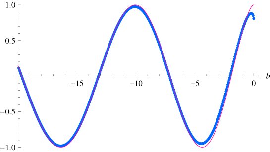
Figure 1: Thick dotted line: the rescaled Stokes multiplier $\frac{i}{2}e^{\frac{\sqrt{\pi}\Gamma(1/3)}{2^{\frac{5}{3}}\Gamma(11/6)}(-b)^{\frac{5}{6}}}\sigma_{0}(b)$ evaluated with our algorithm; thin continuous line: $\cos\left(\frac{\sqrt{\frac{\pi}{3}}\Gamma(1/3)}{2^{5/3}\Gamma(11/6)}(-b)^{\frac{5}{6}}\right)$, i.e. the WKB prediction for the rescaled Stokes multiplier.

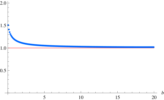
Figure 2: Thick dotted line: the rescaled Stokes multiplier $e^{-\frac{\sqrt{\frac{\pi}{3}}\Gamma(1/3)}{2^{2/3}\Gamma(11/6)}b^{\frac{5}{6}}}\sigma_{0}(b)$ evaluated with our algorithm; thin continuous line: 1, the WKB prediction for the rescaled Stokes multiplier.

We also tested our results against the numerical solution (due to A. Moro and the author) of the Deformed Thermodynamic Bethe Ansatz equations (Deformed TBA), which has been recently introduced by the author [Mas10c], developing the seminal work of Dorey and Tateo [DT99]. The Deformed TBA equations are a set of nonlinear integral equations which describe the exact correction to the WKB asymptotics. The numerical solution of the Deformed TBA equations enable to a-priori set the absolute error in the evaluation of the Stokes multiplier $\sigma_{0}(b)$ rescaled with respect to the exponential factor, shown in (16). Hence, in the range of $-20\leq b\leq 20$ we could verify that we had computed the rescaled $\sigma_{0}(b)$ with an absolute error less than $10^{-8}$.

5 Appendix

The reader expert in anharmonic oscillators theory will skip this Appendix; for her, it will be enough to know that we denote $\sigma_{k}(y,y^{\prime},z)$ the $k-th$ Stokes multipliers of equation (2). Here we review briefly the standard way, i.e. by means of Stokes multipliers, of introducing the monodromy problem for equation (2). All the statements of this section are proved in Appendix A of author’s paper [Mas10a] and in Sibuya’s book [Sib75] .

Lemma 4.

Fix $k\in\mathbb{Z}_{5}=\left\{-2,\dots,2\right\}$ and define a cut in the $\mathbb{C}$ plane connecting $\lambda=y$ with infinity such that its points eventually do not belong to $S_{k-1}\cup\overline{S_{k}}\cup S_{k+1}$. Choose the branch of $\lambda^{\frac{1}{2}}$ by requiring

$$\lim_{\begin{subarray}{c}\lambda\to\infty\\ \arg{\lambda}=\frac{2\pi k}{5}\end{subarray}}{\rm Re}\lambda^{\frac{5}{2}}=+\infty\,,$$

while choose arbitrarily one of the branch of $\lambda^{\frac{1}{4}}$. Then there exists a unique solution $\psi_{k}(\lambda;a,b)$ of equation (5) such that

$$\lim_{\begin{subarray}{c}\lambda\to\infty\\ \left|\arg{\lambda}-\frac{2\pi k}{5}\right|<\frac{3\pi}{5}-\varepsilon\end{subarray}}\frac{\psi_{k}(\lambda;y,y^{\prime},z)}{\lambda^{-\frac{3}{4}}e^{-\frac{4}{5}\lambda^{\frac{5}{2}}+\frac{z}{2}\lambda^{\frac{1}{2}}}}\to 1,\;\forall\varepsilon>0\,.$$ (17)

Definition.

We denote $\psi_{k}$ the k-th subdominant solution or the solution subdominant in the k-th sector.

From the asymptotics (17), it follows that $\psi_{k}$ and $\psi_{k+1}$ are linearly independent. If one fixes the same branch of $\lambda^{\frac{1}{4}}$ in the asymptotics (17) of $\psi_{k-1},\psi_{k},\psi_{k+1}$ then the following equations hold true

$$\frac{\psi_{k-1}(\lambda;y,y^{\prime},z)}{\psi_{k}(\lambda;y,y^{\prime},z)} = \frac{\psi_{k+1}(\lambda;y,y^{\prime},z)}{\psi_{k}(\lambda;y,y^{\prime},z)}+\sigma_{k}(y,y^{\prime},z)\;,$$

$$-i\sigma_{k+3}(y,y^{\prime},z) = 1+\sigma_{k}(y,y^{\prime},z)\sigma_{k+1}(y,y^{\prime},z)\,,\;\forall k\in\mathbb{Z}_{5}\;.$$

Definition.

The entire functions $\sigma_{k}(y,y^{\prime},z)$ are called Stokes multipliers. The quintuplet of Stokes multipliers $\sigma_{k}(y,y^{\prime},z),k\in\mathbb{Z}_{5}$ is called the monodromy data of equation (5).

References

- [CC94] D. V. Chudnovsky and G. V. Chudnovsky. Explicit continued fractions and quantum gravity. Acta Appl. Math., 36(1-2):167–185, 1994.
- [CG09] T. Claeys and T. Grava. Universality of the break-up profile for the KdV equation in the small dispersion limit using the Riemann-Hilbert approach. Comm. Math. Phys., 286(3):979–1009, 2009.
- [DGK09] B. Dubrovin, T. Grava, and C. Klein. On universality of critical behaviour in the focusing nonlinear Schrödinger equation, elliptic umbilic catastrophe and the tritronquée solution to the Painlevé-I equation. J. Nonlinear Sci., 19:57–94, 2009.
- [DT99] P. Dorey and R. Tateo. Anharmonic oscillators, the thermodynamic Bethe ansatz and nonlinear integral equations. J. Phys. A, 32(38):L419–L425, 1999.
- [Dub08] B. Dubrovin. On universality of critical behaviour in Hamiltonian PDEs. volume 224 of Amer. Math. Soc. Transl. Ser. 2, pages 59–109. Amer. Math. Soc., 2008.
- [EG09] A. Eremenko and A. Gabrielov. Analytic continuation of eigenvalues of a quartic oscillator. Comm. Math. Phys., 287(2):431–457, 2009.
- [Elf34] G. Elfving. Über eine Klasse von Riemannschen Flächen und ihre Uniformisierung. Acta Soc. Sci. fenn. N.s. 2, 3:1 – 60, 1934.
- [FIKN06] A. Fokas, A. Its, A. Kapaev, and V. Novokshenov. Painlevé transcendents, volume 128 of Mathematical Surveys and Monographs. American Mathematical Society, 2006. The Riemann-Hilbert approach.
- [Mas10a] D. Masoero. Poles of integrale tritronquee and anharmonic oscillators. A WKB approach. J. Phys. A: Math. Theor., 43(9):5201, 2010.
- [Mas10b] D. Masoero. Poles of integrale tritronquee and anharmonic oscillators. Asymptotic localization from WKB analysis. Nonlinearity, 23:2501 –2507, 2010.
- [Mas10c] D. Masoero. Y-System and Deformed Thermodynamic Bethe Ansatz. arXiv:1005.1046. Accepted for publication in Letters in Mathematical Physics, 2010.
- [Nev32] R. Nevanlinna. Über Riemannsche Flächen mit endlich vielen Windungspunkten. Acta Math., 58(1):295–373, 1932.
- [Olv10] S. Olver. A general framework for solving Riemann-Hilbert problems numerically. Mathematical Institute, Oxford University, Report no. NA-10/5, 2010.
- [Sib75] Y. Sibuya. Global theory of a second order linear ordinary differential equation with a polynomial coefficient. North-Holland Publishing Co., 1975.