Stability of attractive bosonic cloud with van der Waals interaction

Abstract

We investigate the structure and stability of Bose-Einstein condensate of ⁷Li atoms with realistic van der Waals interaction by using the potential harmonic expansion method. Besides the known low-density metastable solution with contact delta function interaction, we find a stable branch at a higher density which corresponds to the formation of an atomic cluster. Comparison with the results of non-local effective interaction is also presented. We analyze the effect of trap size on the transition between the two branches of solutions. We also compute the loss rate of a Bose condensate due to two- and three-body collisions.

I Introduction

Experiments of Bose-Einstein condensation (BEC) with ⁷Li atoms is still a challenging research area as the $s$-wave scattering length ($a_{s}$) is negative, which indicates an attractive atom-atom interaction [1]. A homogeneous condensate with negative scattering length is impossible, as it leads to ever increasing density [2]. As $a_{s}$ is negative, the attractive interaction energy gradually increases with increase in the number of atoms in a small volume and the condensate approaches collapse. However, the situation changes drastically in the presence of an external confinement. A spatially confined BEC may be stable for a small, finite number of atoms [3]. In the presence of a confining potential, the destabilizing effect of the effective negative interaction is balanced by the kinetic pressure of the gas and a metastable condensate can form [1]. For ⁷Li, $a_{s}=-(27.3\pm 0.8)$ Bohr and for T=0, a metastable condensate exists when the number of atoms is less than the critical number, which is roughly 1300 [4], whereas theories predict that BEC can occur in a trap with no more than about 1400 atoms [3,5-7].

During the last decade a number of articles have been published where the properties and stability of the attractive condensate have been discussed in details [3,5-7]. The two- and three-body decay processes near the collapse have also been studied in a number of papers [7,8]. However, all the earlier calculations use the mean-field approximation and the ground state energy is calculated by the Gross-Pitaevskii (GP) energy functional dalfovo . GP theory is based on the pseudopotential form of the atom-atom interaction i.e. a $\delta$-function potential, where the strength of interatomic interaction is absolutely determined by a single parameter $a_{s}$. But due to the presence of the pathological singularity at $|{\vec{x}}|=0$, the Hamiltonian becomes unbound from below and it has been emphasized previously that a $\delta$-function is not suitable as an exact potential in 3D attractive systems geltman ; gao . Again, as the attractive BEC becomes highly correlated near the critical point, uncorrelated GP equation can not take care of the effect of interatomic correlation.

Thus the motivation of the present work is to study the same system using an ab initio many-body method, that is the potential harmonic expansion method ballot ; fabre , with the incorporation of a realistic potential, like the van der Waals potential. The presence of a hard sphere below some cutoff radius and the $-C_{6}/|{\vec{x}}|^{6}$ tail properly take care of the effects of both short-range and long-range correlation and accurately represent the realistic features. We find the commonly known low-density metastable branch and discuss its stability, structure and decay rates due to inelastic two- and three-body collisions. Besides the known solution, we also find another branch of solution at a higher density. Due to the use of the realistic van der Waals interaction in the many-body calculation, we have a deep attractive well on the left side of the metastable region in the effective potential. In the standard GP theory, the metastable region just vanishes at the critical point and the whole condensate collapses into the singular well and the fate of the condensate is not predicted further. However, in our calculation the metastable condensate leaks through the intermediate barrier and settles down in the extremely narrow (width $\sim 0.05\mu m$) well. The atoms become highly correlated and due to high two-body and three-body collisions, atoms form a cluster. This corresponds to the high-density branch. In the present communication, we investigate the transition between the two branches of solutions as a function of the number of atoms and their dependence on the trap size. We also calculate decay rates of the condensate due to two- and three-body collisions. In other articles luca , the existence of a similar type of new stable branch has been reported, which is intermediate in density between the dilute metastable state and the collapsed state. This is described as the effect of use of non-local interaction in the GP theory. It has been pointed out that for ⁷Li system, the scattering cross-section has a momentum dependence and the effective interaction is non-local, changing from attractive to repulsive at a characteristic range $r_{e}$. They calculated the properties of the attractive condensate by the variational technique. Using a Gaussian trial wavefunction they minimized the quantum action.

In the present communication, we also compare our results with those obtained using the non-local interaction. A road map of the present study is given below. Sec.II contains the many-body approach used in this work, which is based on the potential harmonic expansion method. Sec.III presents the calculation with a non-local interaction. Sec. IV contains a comparison of the structure and stability of the bosonic system of both the low- and high-density branches obtained from two different theoretical calculations and the discussion of the many-body effect. Sec.V provides a summary of our results and their conclusions.

II Many-body calculation: (a) Potential harmonics basis

We consider a system of A=(N+1) identical spinless bosons (each of mass m) confined in an external trapping potential $U_{trap}({\vec{x}}_{j})$ and interacting via a two-body potential V($\vec{x}_{i}-\vec{x}_{j}$), $\vec{x}_{i}$ being the position vector of the $i$-th particle. The corresponding Schrödinger equation is written as

$$\Big{[} - \frac{\hbar^{2}}{2m}\sum_{i=1}^{A}\nabla_{i}^{2}+\sum_{i=1}^{A}U_{trap}(\vec{x}_{i})+$$ (1)

$$\sum_{i,j>i}^{A}V(\vec{x}_{i}-\vec{x}_{j})-E\Big{]}\psi(\vec{x}_{1},...,\vec{x}_{A})=0.$$

We define N Jacobi vectors as

$$\vec{\zeta}_{i}=\sqrt{\frac{2i}{i+1}}\left(\vec{x}_{i+1}-\frac{1}{i}\sum_{j=1}^{i}\vec{x}_{j}\right),\hskip 14.22636pt(i=1,...,N).$$ (2)

The center of mass is $\vec{R}=\sum_{i=1}^{A}\vec{x}_{i}/A$. Since the labelling of particles is arbitrary, we choose the relative separation of $(i,j)$ interacting pair ($\vec{x}_{ij}=\vec{x}_{i}-\vec{x}_{j}$) as $\vec{\zeta}_{N}$. We next define the hyperradius $r$ of the set of N Jacobi vectors through ballot

$$r^{2}=\sum_{i=1}^{N}\zeta_{i}^{2}=\frac{2}{A}\sum_{i,j>i}x_{ij}^{2}=2\sum_{i=1}^{A}r_{i}^{2}\hskip 8.5359pt,$$ (3)

where $\vec{r}_{i}=\vec{x}_{i}-\vec{R}$ is the position vector of the $i$-th particle from the center of mass of the system. In this way the relative motion of the bosons is described by

$$\Big{[} - \frac{\hbar^{2}}{m}\sum_{i=1}^{N}\nabla_{\zeta_{i}}^{2}+V_{trap}(r)+$$ (4)

$$V_{int}(\vec{\zeta}_{1},...,\vec{\zeta}_{N})-E_{R}\Big{]}\psi(\vec{\zeta}_{1},...,\vec{\zeta}_{N})=0,$$

where E_R is the energy of the relative motion. In the present work $U_{trap}({\vec{x}}_{i})=\frac{1}{2}m\omega^{2}|{\vec{x}}_{i}|^{2}$ is a spherically symmetric harmonic oscillator potential and consequently

$$\sum_{i=1}^{A}U_{trap}({\vec{x}}_{i})=\frac{1}{4}m\omega^{2}r^{2}+\frac{1}{2}mA\omega^{2}R^{2}.$$ (5)

The first term on the right side is the effective trap potential $V_{trap}(r)$ for the relative motion and the second term is the trap potential of the center of mass motion. The equation for the center of mass motion separates completely and is simply the equation for a three dimensional harmonic oscillator. The total energy of the system is thus $(E_{R}+\frac{3}{2}\hbar\omega)$. In Eq. (4), $V_{int}$ is the sum of all pair-wise interactions, expressed in terms of the Jacobi vectors. In our approach we consider that when $(ij)$ pair interacts, the rest of the bosons are inert spectators. So we define a hyperradius $\rho_{ij}$ for the remaining (N-1) noninteracting bosons as fabre

$$\rho_{ij}=\left[\sum_{k=1}^{N-1}\zeta_{k}^{2}\right]^{1/2},$$ (6)

so that $r^{2}=x_{ij}^{2}+\rho_{ij}^{2}$. The hyperangle $\phi$ is introduced through $x_{ij}=r\cos\phi$ and $\rho_{ij}=r\sin\phi$. Besides $r,\phi,\vartheta,\varphi$ (where $\vartheta$ and $\varphi$ are the polar angles of $\vec{x}_{ij}$), there are $(3N-4)$ remaining variables. These are constituted by $2(N-1)$ polar angles associated with ($\vec{\zeta}_{1},...,\vec{\zeta}_{N-1}$) and $(N-2)$ angles defining their relative lengths and collectively denoted by $\Omega_{N-1}^{(ij)}$, called hyperangles in the $3(N-1)$-dimensional space. The corresponding form of Laplace operator can be found in ballot . In the potential harmonics expansion method (PHEM), $\psi$ is decomposed into Faddeev components, $\phi_{ij}$ for the $(ij)$ interacting pair as,

$$\psi=\sum_{i,j>i}^{A}\phi_{ij}.$$ (7)

Then Eq. (4) can be written as

$$(T+V_{trap}-E_{R})\phi_{ij}=-V(x_{ij})\sum_{k,l>k}^{A}\phi_{kl},$$ (8)

where $T=-\frac{\hbar^{2}}{m}\sum_{i=1}^{N}\nabla^{2}_{\vec{\zeta}_{i}}$. Note that the assumptions that correlations higher than two-body ones in $\psi$ are negligible and that the angular and hyperangular momenta of the system are contributed by the interacting pair only chak1 , make the Faddeev component $\phi_{ij}$ independent of the coordinates of all the particles, other than the interacting pair ballot . Thus $\phi_{ij}=\phi_{ij}(\vec{x}_{ij},r)$. With this assumption we expand $\phi_{ij}$ in the subset of hyperspherical harmonics (HH) necessary for the expansion of V($\vec{x}_{ij}$). Thus,

$$\phi_{ij}(\vec{x}_{ij},r)=r^{\frac{-(3N-1)}{2}}\sum_{K}\mathcal{P}_{2K+l}^{lm}(\Omega^{ij}_{N})u_{K}^{l}(r).$$ (9)

This subset of HH is called the potential harmonics (PH) basis and is denoted by $\{\mathcal{P}_{2K+l}^{lm}(\Omega^{ij}_{N})\}$; $\Omega^{ij}_{N}$ denotes the set of hyperangles in 3N dimensional space with the interacting pair uniquely identified as above. Note also that $\mathcal{P}_{2K+l}^{lm}(\Omega^{ij}_{N})$ is independent of ($\vec{\zeta}_{1},...,\vec{\zeta}_{N-1}$) and thus no contribution to the orbital and hyper angular momenta of the condensate comes from the remaining $(N-1)$ noninteracting bosons. Thus the total orbital angular momenta of the condensate and its projection are simply those of the interacting pair, viz. $l$ and $m$ respectively. The complete analytic expression for $\mathcal{P}_{2K+l}^{lm}(\Omega^{ij}_{N})$ can be found in fabre . Substitution of Eq. (9) into Eq. (8) and subsequent projection on a particular PH gives chak1

$$\Big{[} - \frac{\hbar^{2}}{m}\frac{d^{2}}{dr^{2}}+\frac{\hbar^{2}}{m}\frac{{\cal L}_{K}({\cal L}_{K}+1)}{r^{2}}+V_{trap}(r)-E_{R}\Big{]}u_{K}^{l}(r)$$ (10)

$$+ \sum_{K^{\prime}}f_{K^{\prime}l}^{2}V_{KK^{\prime}}(r)u_{K^{\prime}}^{l}(r)=0,$$

where $V_{KK^{\prime}}(r)$ is the potential matrix and is given by,

$$V_{KK^{\prime}}(r)=\int{\mathcal{P}}_{2K+l}^{{lm}^{*}}(\Omega^{ij}_{N})V(x_{ij}){\mathcal{P}}_{2K^{\prime}+l}^{lm}(\Omega^{ij}_{N})d\Omega_{N}^{ij}.$$ (11)

The quantities $\mathcal{L}_{K}$ and $f^{2}_{Kl}$ are given by

$$\begin{array}[]{rcl}{\cal L}_{K}&=&2K+l+\frac{3N-3}{2}\\ f_{Kl}^{2}&=&\sum_{k,l>k}<{\mathcal{P}}_{2K+l}^{lm}(\Omega^{ij}_{N})|{\mathcal{P}}_{2K+l}^{lm}(\Omega^{kl}_{N})>,\\ \end{array}$$ (12)

the latter being the overlap of the PH for the $(ij)$-partition (corresponding to only the $(ij)$-pair interacting) with the sum of PH for all partitions. The quantum number $K$ in Eq. (10) is the hyperspherical (grand orbital) quantum number in the $3N$ dimensional space ballot ; fabre , analogous with the orbital angular momentum in three dimensional space. The ordinary orbital angular momentum of the system and its projection are $l$ and $m$, as indicated earlier. All other intermediate angular momentum quantum numbers of the system take zero eigen values, due to the choice of the PH basis. Thus the choice of the PH basis reduces the complications of the many-body system immensely. Eq. (10) can be put in a symmetric form as

$$\Big{[} - \dfrac{\hbar^{2}}{m}\dfrac{d^{2}}{dr^{2}}+\dfrac{\hbar^{2}}{mr^{2}}\{{\cal L}({\cal L}+1)+4K(K+\alpha+\beta+1)\}$$

$$+ V_{trap}(r)-E_{R}\Big{]}U_{Kl}(r)$$

$$+ \sum_{K^{\prime}}f_{Kl}V_{KK^{\prime}}(r)f_{K^{\prime}l}U_{K^{\prime}l}(r)=0,$$

where ${\cal L}=l+(3A-6)/2$, $U_{Kl}(r)=f_{Kl}u_{K}^{l}(r)$, $\alpha=\frac{3A-8}{2}$ and $\beta=l+\frac{1}{2}$.

III Many-body calculation: (b) Incorporation of two-body correlation function

In the experimentally achievable BEC, the average interparticle separation is much larger than the range of two-body interaction. This is indeed required to prevent atomic three-body collisions and formation of molecules. Moreover, the energy of the interacting pair is extremely small. Thus the two-body interaction is generally represented by the $s$-wave scattering length ($a_{s}$). In the GP picture, the effective interaction is given in terms of $a_{s}$ alone, making the results independent of the shape of the interatomic potential. Hence, a positive value of $a_{s}$ gives a repulsive condensate and a negative $a_{s}$ gives an attractive condensate. However, a realistic interatomic interaction, like the van der Waals potential, is always associated with an attractive $-1/|{\vec{x}}_{ij}|^{6}$ tail at larger separations and a strong repulsion at short separations. Depending on the nature of these two parts, $a_{s}$ can be either positive or negative pethick . For a given two-body potential $V(x_{ij})$ having a finite range, $a_{s}$ can be obtained by solving the zero-energy two-body Schrödinger equation for the wave function $\eta(x_{ij})$

$$-\frac{\hbar^{2}}{m}\frac{1}{x_{ij}^{2}}\frac{d}{dx_{ij}}\left(x_{ij}^{2}\frac{d\eta(x_{ij})}{dx_{ij}}\right)+V(x_{ij})\eta(x_{ij})=0.$$ (14)

The asymptotic part of $\eta(x_{ij})$ has the form $(c_{1}x_{ij}+c_{2})$ and the corresponding $s$-wave scattering length is given by $a_{s}=-\frac{c_{2}}{c_{1}}$.

Now the rate of convergence of the PH expansion in Eq. (9) is very slow. This can be understood from the fact that the leading term of this basis, viz. the term with $K=0$, is a non-zero constant, while $\phi_{ij}$ must be vanishingly small for small values of $x_{ij}$ due to the strong short-range repulsion of $V(x_{ij})$. Consequently a large number of terms is needed to represent $\phi_{ij}$ faithfully for small values of $x_{ij}$. The rate of convergence is improved dramatically by introducing a short-range correlation function in the expansion basis CDLin , that represents the true nature of $\phi_{ij}(x_{ij})$ as $x_{ij}\rightarrow 0$. In the experimental BEC, the energy of the interacting pair (which is $\sim\hbar\omega$) is negligible compared with the depth of interaction potential $V(x_{ij})$ (which is of the order of typical atomic energy scale). Thus $\eta(x_{ij})$ is a good representation of the short-range behavior of $\phi_{ij}(x_{ij})$. Hence we use $\eta(x_{ij})$ as a short-range correlation function in the PH expansion, to enhance its rate of convergence chak2 :

$$\phi_{ij}(\vec{x}_{ij},r)=r^{\frac{-(3N-1)}{2}}\sum_{K}\mathcal{P}_{2K+l}^{lm}(\Omega^{ij}_{N})u_{K}^{l}(r)\eta(x_{ij}).$$ (15)

As $\eta(x_{ij})$ correctly reproduces the short separation behavior of the interacting-pair Faddeev component, convergence rate of the PH expansion for the residual part of $\phi_{ij}$ is quite fast. Validity of this statement has been tested in numerical calculations. In an actual calculation, we solve Eq. (14) for the zero energy two-body wave function $\eta(x_{ij})$ in the chosen two-body potential $V(x_{ij})$, after adjusting the hard core radius ($r_{c}$), such that $a_{s}$ has the desired value Das1 . This $\eta(x_{ij})$ is then used in Eq. (15).

Then the potential matrix becomes

$$V_{KK^{\prime}}(r) = (h_{K}^{\alpha\beta}h_{K^{\prime}}^{\alpha\beta})^{-\frac{1}{2}}\int_{-1}^{+1}\Big{\{}P_{K}^{\alpha\beta}(z)V\left(r\sqrt{\frac{1+z}{2}}\right)$$ (16)

$$P_{K^{\prime}}^{\alpha\beta}(z)\eta\left(r\sqrt{\frac{1+z}{2}}\right)w_{l}(z)\Big{\}}dz.$$

where $P_{K}^{\alpha\beta}(z)$ is the Jacobi polynomial, whose norm and weight function are $h_{K}^{\alpha\beta}$ and $w_{l}(z)$ respectively abram . We restrict the K-sum in Eq. (15) to an upper limit $K_{max}$ from the requirement of convergence. Finally we solve the set of coupled differential equations (CDE), Eq. (13), by hyperspherical adiabatic approximation das2 . The total energy of the system is obtained by adding energy of the center of mass motion ($3\hbar\omega/2$) to $E_{R}$. The wave function of the condensate in the physical space can be obtained from $U_{Kl}(r)$, using Eqs. (7) and (9) and the ralations between hyperspherical and physical coordinates.

IV GP theory with non-local interaction

In the standard treatment of alkali-metal atoms, the interatomic interaction is chosen as a local form, i.e., momentum independent. The effective zero-range pseudopotential has the form $V({\vec{x}})=g\delta^{3}({\vec{x}})$, where $g=\frac{4\pi\hbar^{2}a_{s}}{m}$. However, this is not correct when the scattering cross-section has a significant momentum dependence. This implies that the effective interaction is non-local, changing from attractive to repulsive at a characteristic range $r_{e}$. The system of ⁷Li atoms exhibit such momentum dependence and the effective ⁷Li-⁷Li interaction can be written as [11]

$$V(k)=\frac{4\pi\hbar^{2}}{m}[a_{r}+(a_{s}-a_{r})f(kr_{e})]$$ (17)

where $a_{s}$ corresponds to the attractive potential and has the value $a_{s}=-27.3$ Bohr, whereas the repulsive contribution is modeled by a local positive term with $a_{r}=6.6$ Bohr and $r_{e}$ = $10^{3}$ Bohr. The shape function $f(x)$ may be chosen as a Lorenzian $f(x)=(1+x^{2})^{-1}$. In real space the effective inter-atomic potential then reads

$$V({\vec{x}})=\frac{4\pi\hbar^{2}a_{s}}{m}\delta^{3}({\vec{x}})+\frac{\hbar^{2}(a_{s}-a_{r})}{mr_{e}^{2}}\ {e^{-|{\vec{x}}|/r_{e}}\over|{\vec{x}}|}\;.$$ (18)

This potential appears in the nonlocal GP energy functional

$$E=\int\phi^{*}(\vec{x})\left[-{\hbar^{2}\over 2m}\nabla^{2}+U_{trap}(|{\vec{x}}|)\right]\phi(\vec{x})\ d^{3}\vec{x}$$

$$+{1\over 2}\int|\phi({\vec{x}})|^{2}V({\vec{x}}-{\vec{x}}^{\prime})|\phi({\vec{x}}^{\prime})|^{2}\ d^{3}\vec{x}\ d^{3}\vec{x}^{\prime}\;,$$ (19)

where $\phi({\vec{x}})$ is the spherically-symmetric GP wave function. In earlier calculations luca the variational ansatz of the wave function is chosen as

$$\phi(|\vec{x}|)=N^{1/2}\frac{1}{\pi^{3/4}\sigma^{3/2}}{\rm exp}\left\{-\frac{|{\vec{x}}|^{2}}{2\sigma^{2}a_{0}^{2}}\right\}$$ (20)

where $\sigma$ is the variational parameter, $\sigma a_{0}$ being the width of the condensate with $a_{0}=\sqrt{\frac{\hbar}{m\omega}}$ the characteristic length of the harmonic trap. In this way the energy $E$ of the system becomes luca

$$E(\sigma)={N\hbar\omega\over 4}\left[\frac{3}{\sigma^{2}}+3\sigma^{2}+2N\left(\frac{\gamma_{r}}{\sigma^{3}}+\frac{\tau_{1}}{\sigma}-\tau_{2}g(\chi\sigma)\right)\right]\;,$$ (21)

with $\gamma_{r}=(2/\pi)^{1/2}a_{r}/a_{0}$, $\tau_{1}=(2/\pi)^{1/2}a_{0}(a_{s}-a_{r})/r_{e}^{2}$, $\chi=2^{-1/2}a_{0}/r_{e}$, $\tau_{2}=a_{0}^{2}(a_{s}-a_{r})/r_{e}^{3}$ and $g(x)={\rm exp}(x^{2})[1-{\rm erf}(x)]$, ${\rm erf}(x)$ is the error function. The extrema of $E(\sigma)$ are obtained from the following expression,

$$N=(1-\sigma^{4}){\left[-\gamma_{r}\sigma^{-1}-\frac{\tau_{1}\sigma}{3}+\frac{2\chi\tau_{2}\sigma^{3}}{3\sqrt{\pi}}-\frac{2\chi^{2}\tau_{2}\sigma^{4}g(\chi\sigma)}{3}\right]}^{-1}$$ (22)

which actually gives the number of bosons as a function of the scaled size $\sigma$ of the cloud. Depending on the choice of parameters and the number of atoms, this equation either has one root or three roots. When three solutions are present, one corresponds to the low-density metastable solution (which we expect for local interaction), one corresponds to the high density stable solution (which is the effect of non-locality) and the middle one corresponds to an unstable state (i.e. local maximum). The variational results for different trap sizes are discussed in the result section.

V Results

We consider the experiment on ⁷Li condensate at Rice University iju , for which $a_{s}=-27.3$ Bohr. We take $a_{0}$ as the unit of length and energy is expressed in units of the oscillator energy quanta $\hbar\omega$. The trap size corresponding to the Rice University experiment is $a_{0}=3.0\mu m.$ For the many-body calculation, we choose the van der Waals potential, whose short range repulsion is characterized by a hard core of radius $r_{c}$ and the long range part is described by an attractive tail $-C_{6}/|{\vec{x}}_{ij}|^{6}$, where $C_{6}$ is the strength parameter which is known from experiments. Choice of a realistic interatomic interaction like the van der Waals potential is very important, as it has been shown that the shape-independent approximation is not valid in typical laboratory BECs chak3 . In the local mean-field description the two-body interaction is usually represented by the $s$-wave scattering length $a_{s}$. To mimic the ⁷Li trap of Rice University, our chosen parameters are $C_{6}=1.71487\times 10^{-12}$ o.u. and $r_{c}=5.3378\times 10^{-4}$ o.u., which reproduce the experimental value of $a_{s}$. With these sets of parameters we solve the set of coupled differential equations by the hyperspherical adiabatic approximation (HAA) das2 . We assume that the hyperradial motion is slow in comparison with the hyperangular motion. Hence, for a fixed value of $r$, the equation for the hyperangular motion can be solved adiabatically. The energy eigen value of this equation is a parametric function of $r$ and provides an effective potential for the hyperradial motion. In the HAA prescription, the lowest lying such potential is used for the ground state of the system. Although Eq. (13) involves the hyperradius $r$ only, the hyperangular motion appears through the coupling matrix $V_{Kk^{\prime}}(r)$. Solution of the hyperangular motion for a fixed value of $r$ is equivalent to diagonalizing the hyperangular Hamiltonian in the potential harmonics basis, i.e. diagonalizing the potential matrix $V_{KK^{\prime}}(r)$ together with the hypercentrifugal term of Eq. (13). The lowest eigenvalue of this matrix, $\omega_{0}(r)$, is the effective potential in the hyperradial space, in which collective motion of the condensate takes place. Thus the energy and wave function of the condensate is obtained by solving the equation for hyperradial motion

$$\left[-\frac{\hbar^{2}}{m}\frac{d^{2}}{dr^{2}}+\omega_{0}(r)+\sum_{K=0}^{K_{max}}|\frac{d\chi_{K0}(r)}{dr}|^{2}-E_{R}\right]\zeta_{0}(r)=0\hskip 8.5359pt,$$ (23)

where the third term is the overbinding correction term das2 and $\chi_{K0}$ is the K-th component of the column vector corresponding to the eigenvalue $\omega_{0}(r)$. Energy and wave function of the system are obtained by solving Eq. (23) numerically, subject to appropriate boundary conditions. The partial wave $U_{Kl}(r)$ appearing in Eq. (13) is given in HAA as $U_{Kl}(r)\approx\zeta_{0}(r)\chi_{K0}(r)$ das2 .

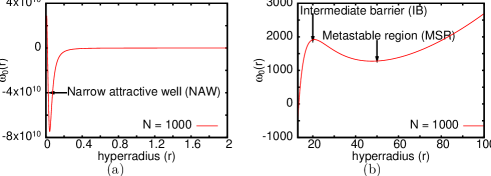
Figure 1: (Color online) Plot of effective potential $\omega_{0}(r)$ in o.u. against $r$ in o.u. for 1000 ⁷Li atoms with $a_{0}=3.0\mu m$. Panel (a) shows the narrow attractive well, while panel (b) displays the metastable region in detail. Note the different horizontal and vertical scales in the two panels.

In Fig. 1 we plot the effective potential, $\omega_{0}(r)$ for N = 1000 atoms of ⁷Li, the condensate being metastable as N$<$N_cr. For N$<$N_cr, the intermediate metastable region (MSR) of $\omega_{0}(r)$ is bounded by the high wall of the external trap on the right side and on the left by an intermediate barrier (IB) [panel (b)]. On the left of the IB, a very deep narrow attractive well (NAW) appears which is again followed by a steeply increasing repulsive wall, as $r$ decreases [panel (a)]. The existence of a strong repulsive core near the origin ($r\rightarrow 0$) is in sharp contrast to the GP mean-field picture with local interaction and is the immediate reflection of the use of realistic van der Waals interaction in quantum many-body calculation. In the GP picture, negative $a_{s}$ presents a singular attraction (with no repulsive core) near the origin. The combination of repulsive core and NAW in the present approach, prevents the Hamiltonian from being unbound from below. As the number of atoms increases towards the critical number, the height of the intermediate barrier decreases, the NAW becomes more negative and narrow. At N = N_cr, the MSR along with the intermediate barrier disappear, with the local maximum of the IB and the local minimum of the MSR merging to form a point of inflexion Das1 . The value of N where this occurs is N_cr. As N becomes larger than N_cr, all the atoms get trapped in the NAW, giving rise to a cluster state resulting from the increased interatomic correlations and two- and three-body collisions. The release of binding energy is observed as a burst of energy in experiments. This is the collapse scenario in the present approach.

Thus the qualitative features of the pre-collapse scenario are in fair agreement with the GP local mean-field picture away from the critical number. When N = N_cr, the energy per particle becomes $-\infty$ in the local GP method, and the Hamiltonian becomes unbound from below. However, in our many-body calculation the Hamiltonian has a lower bound due to the presence of a hypercentrifugal barrier as $r\rightarrow 0$ along with the use of a realistic interatomic interaction with a repulsive core of finite size. In the post-collapse state the atoms accumulate in the narrow attractive well and form clusters.

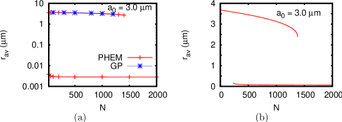
Figure 2: (Color online) Size of the condensate as a function of the number of ⁷Li atoms using PHEM with van der Waals interaction and GP with local interaction (having same $a_{s}$) [panel (a)], and GP with non-local interaction [panel (b)].

We calculate the size of the condensate as a function of the number of ⁷Li atoms, for the choice of the parameters mentioned earlier. We define the average size of the condensate ($r_{av}$) as the root mean square distance of individual atoms from the center of mass and is given by Das1

$$r_{av}=\left\langle\frac{1}{A}\sum_{i=1}^{A}(\vec{x}_{i}-\vec{R})^{2}\right\rangle^{1/2}=\frac{<r^{2}>^{1/2}}{\sqrt{2A}}$$ (24)

where $\vec{R}$ is the center of mass coordinate. We present average size of the condensate calculated by PHEM in panel (a) of Fig. 2. The upper branch corresponds to the metastable condensate. With increase in particle number, the total attractive interaction increases as $\frac{N(N-1)}{2}$, the system contracts and $r_{av}$ decreases as expected. For comparison we present in panel (a) the results of the GP equation with contact interaction, i.e. with local interaction. The lower branch, which corresponds to the high-density stable branch in the deep attractive well, starts from N=20. In the GP mean-field approach with local interaction, there is no other stable branch after collapse as the whole condensate falls into the singular well. In our calculation we find that the size of the condensate in the deep attractive well is of the order of 0.003 $\mu m$, which is the order of the size of the atomic cluster. This clearly indicates that the metastable condensate forms clusters due to high two-body and three-body collisions within an extremely narrow well of width $\sim$ 0.05 $\mu m$. However, the transition from upper branch to lower branch is discontinuous. In panel (b) of Fig. 2, we present results for the same trap but with non-local interaction as described in Sec.III. The quantity $\sigma a_{0}$ in Eq. (20) is basically the average size of the condensate and is denoted by $r_{av}$ in panel (b) of Fig. 2. The variational parameter $\sigma$ is calculated as a function of the number of bosons using the algebraic equation [Eq. (22)]. The effective potential energy $E(\sigma)$ [Eq. (21)] has the same qualitative features as the many-body effective potential $\omega_{0}(r)$. Unlike the GP effective potential with local interaction, (having one local minimum), the use of non-local interaction in the calculation of effective potential offers an additional absolute minimum together with the local minimum. This absolute minimum corresponds to the high-density stable solution whereas the local minimum corresponds to the usual metastable solution. The transition between the low-density and high-density branches is again discontinuous as observed in many-body calculation. However, unlike panel (a) of Fig. 2, where the high-density stable branch appears from quite small values of N = 20, in panel (b), the lower branch starts from N $\simeq$ 234. This disagreement is due to the fact that the origin of non-locality and the occurrence of absolute minimum is different in the two approaches. In the many-body calculation the effect of non-locality is inherent due to the presence of hypercentrifugal repulsion (arising from the many-body treatment) and the use of van der Waals potential with a finite range hard core part whereas in the other approach the non-locality is created by assuming that the attractive potential has a finite range $r_{e}$ together with a local positive term defined by high-energy scattering length $a_{r}>0$. This is reflected by the presence of a non-local minimum in the effective interaction.

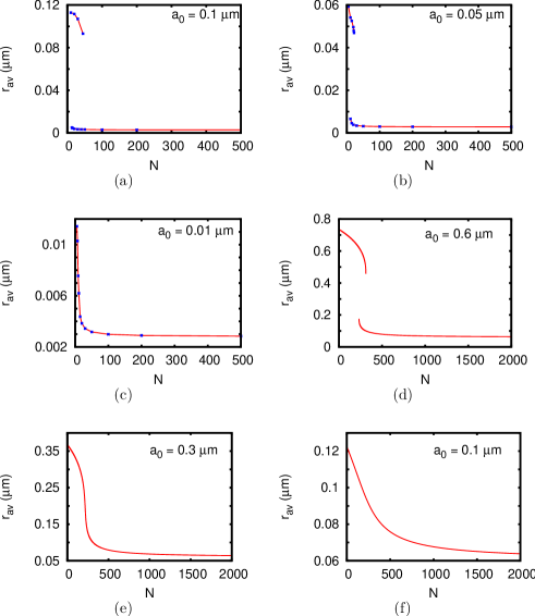
Figure 3: (Color online) Size of the condensate as a function of the number of ⁷Li atoms using PHEM [panels (a) – (c)] and GP with non-local interaction [panels (d) – (f)]. Note that in panels (a) - (c), the horizontal axis is upto $N=500$, to show the small $N$ part prominently. Calculated values of $r_{av}$ for $N$ above $500$ remain practically constant for PHEM.

Next, to study the nature of discontinuity between the two branches of solution, we repeat our calculation for other trap sizes. We plot the PHEM results in panels (a) – (c ) of Fig. 3 with $a_{0}=0.1\mu m$ ($\omega=907.88$kHz), $a_{0}=0.05\mu m$ ($\omega=3.63$MHz) and $a_{0}=0.01\mu m$ ($\omega=90.79$MHz). We observe that by reducing the trap size the discontinuity is strongly reduced and at $a_{0}=0.01\mu m$, the discontinuity disappears. There is a smooth evolution from a dilute cloud to a less dilute cloud. We also observe that the size is almost independent of the trap size for $N>200$, as expected for clusters. For comparison, in panels (d) – (f) of Fig. 3, we plot the variational results with non-local interaction for various trap sizes $a_{0}=0.6\mu m$, $a_{0}=0.3\mu m$ and $a_{0}=0.1\mu m$.
We get almost same qualitative pictures as shown in panel (a) – (c) of Fig. 3; reducing the trap size, the discontinuity is reduced and at $a_{0}=0.1\mu m$, the metastable branch disappears. However, the quantitative disagreement between many-body results and variational results with non-local interaction is again attributed to the different origin of non-locality in the effective potential. In the variational calculation with non-local interaction, the discontinuity disappears at $a_{0}=0.1\mu m$ whereas the corresponding trap size in the many-body calculation is $a_{0}=0.01\mu m$. However, in both cases we observe that the size of the denser cloud is independent of large N, which implies that the atoms are being self-trapped in the non-local minimum.

For the case of a spherical trap with trap size $a_{0}=3.0\mu m$, we fail to find the metastable numerical solutions beyond N $\simeq 1430$ atoms. The instability occurs as the number of atoms increases, the net attractive interaction between atoms becomes dominant and kinetic energy can no longer stabilize the wave function. In the mean-field approach it has already been pointed out that the transition to an unstable state may occur due to quantum tunnelling. This tunnelling is similar to the ordinary quantum tunnelling and its rate can be calculated by the semiclassical formula. As this rate is quite small, neglecting tunnelling we consider only the loss rates due to two-body dipolar collisions and three-body recombination collisions.

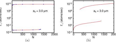
Figure 4: (Color online) Loss rate due to two- and three-body collisions as a function of the number of ⁷Li atoms using PHEM [panel (a)] and GP with non-local interaction [panel (b)].

The total loss rate is given by

$$\Gamma_{L}=K\int d^{3}\vec{x}|\phi(\vec{x})|^{4}+L\int d^{3}\vec{x}|\phi(\vec{x})|^{6}$$ (25)

where two-body dipolar loss rate coefficient $K=1.2\times 10^{-2}\mu{\rm m}^{3}{\rm sec}^{-1}$ and the three-body recombination loss rate coefficient $L=2.6\times 10^{-4}\mu{\rm m}^{6}{\rm sec}^{-1}$ moerdijk . $\phi(\vec{x})$ is the condensate wave function. This is simply given by Eq. (20) for the non-local GP approach. For the many-body approach, the wave function $\psi$ is initially obtained as a function of the Jacobi coordinates. It is then transformed into a function of position vectors $\{{\vec{x}}_{1},{\vec{x}}_{2},...,{\vec{x}}_{A}\}$ of $A$ particles. Finally, the one-body density is obtained by integrating $|\psi|^{2}$ over all ${\vec{x}}_{i}$, except one. This one-body density is used for $|\phi({\vec{x}})|^{2}$ in Eq. (25). It is already known that in case of a negative scattering length, the rapid increase in the density of atoms and large increase in the net attractive interaction for a large number of atoms, result in a very large loss rate near the critical point. Thus for the unique metastable branch in GP mean-field picture with local interaction, the loss rate increases very fast with the increase in the number of atoms [7]. However, due to the presence of the deep attractive well in the many-body picture, we calculate the loss rate for both the branches and observe the discontinuity. By using condensate wave function as described above, we calculate $\Gamma_{L}$ by using Eq. (25) and the results are plotted in panel (a) of Fig. 4. The lower branch corresponds to the metastable region. As the metastable region is flatter compared to the NAW, although the atoms are correlated, the probability of two or more atoms to come very close is relatively small. Thus the loss rate is initially small and increases with increase in atom number. The upper branch accounts for the loss rate in the deep narrow attractive well. As all the atoms are now confined within a very narrow and deep well, they suffer vigorous two- and three-body collisions and the calculated loss rate is much higher than the same calculated in the metastable region. The transition between these two branches is again discontinuous. In panel (b) of Fig. 4 we plot $\Gamma_{L}$ calculated using variational trial wave function of Eq. (20) using non-local interaction. Substitution of trial wave function Eq. (20) in Eq. (25), leads to

$$\Gamma_{L}(N)=\frac{KN^{2}}{(2\pi)^{3/2}a_{0}^{3}\sigma^{3}}+\frac{LN^{3}}{(3\pi^{2})^{3/2}a_{0}^{6}\sigma^{6}}.$$ (26)

In this formula, N is related to $\sigma$ through Eq. (22). The existence of low-density metastable branch and high-density stable branch which are separated by an intermediate unstable branch is also reflected in Fig. 4. It is in sharp contrast to the existence of a unique metastable branch in the mean-field approach with local potential. For the sake of completeness, in Fig. 5 we plot the loss rate for traps of different sizes.

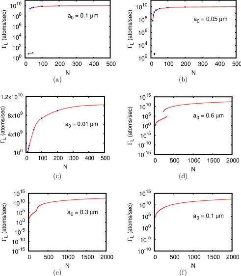
Figure 5: (Color online) Loss rate due to two- and three-body collisions as a function of the number of ⁷Li atoms using PHEM [panels (a) – (c)] and GP with non-local interaction [panels (d) – (f)]. Note that in panels (a) - (c), the horizontal axis is upto $N=500$, to show the small $N$ part prominently. Calculated values of $\Gamma_{L}$ for $N$ above $500$ remain practically constant for PHEM.

VI Conclusions

In summary, we have analyzed the stability of the attractive Bose-Einstein condensate of ⁷Li atoms in a harmonic trap using an ab initio quantum many-body calculation incorporating realistic van der Waals interaction and all possible two-body correlations. Unlike the single metastable condensate arising from the GP mean-field theory with local interaction, we observe that the atomic cloud may exist in different states. In addition to the commonly known low density metastable BEC state, we find a high density stable solution, which corresponds to the cluster state of the lithium atoms. Between these two minima, there is a maximum of the effective potential, which does not correspond to any stable physical state of the Bose gas. The local GP approach produces only the metastable solution, together with an intermediate barrier (local maximum), but the effective potential has no lower bound on the left of the intermediate barrier. Indeed there is a pathological singularity at the origin, which only produces a pathological collapse (not leading to any physical solution). The effect of a non-local momentum dependent interaction (replacing the local contact interaction) in the GP approach was investigated in earlier works luca using a variational ansatz. The results of this non local GP approach agree qualitatively with our present observations. The lack of quantitative agreement is attributed to the difference in the origins of non-locality in the two approaches. We have investigated the average size of the bosonic system, as also the loss rates due to two- and three-body collisions for both the metastable BEC state and the collapsed cluster state. In general these quantities lie on separate branches for the two states. For larger trap lengths, the two branches are unconnected. But there is a continuous transition for very tight traps. The local GP approach produces only one branch, corresponding to the metastable state. The local GP uses an attractive contact interaction for the ⁷Li condensate. This causes a pathological singularity at the origin, preventing any stable collapsed state. The non local GP approach uses a non-local potential, which is attractive at larger separations, but has a repulsive contact interaction as $r\rightarrow 0$. Hence there is no pathological singularity and the effective potential becomes strongly repulsive as $r\rightarrow 0$. This gives rise to the stable high density branch. In the PHEM approach, the realistic van der Waals (vdW) potential is used. This has a very strong repulsion at short separations and an attractive $1/|{\vec{x}}_{ij}|^{6}$ long tail. The strongly repulsive core of the vdW potential, together with the hypercentrigugal repulsion, arising from the PHEM approach, produces a repulsive core followed by a deep attractive well as one moves away from the origin in the effective potential, $\omega_{0}(r)$. Thus both the PHEM and the non local GP approaches produce the same qualitative results. However, quantitative differences exist due to different origins of non-locality in these two approaches. While, non-locality in the many-body approach arises from the use of vdW potential with a repulsive core and the hypercentrifugal repulsion, that in the non local GP approach is built in the choice of the two-body potential.

Although the presence of an intermediate state has already been established in earlier works where GP mean-field theory has been employed with non-local interaction luca , the effect of the short-range behavior of realistic interatomic potential on the intermediate state has not been investigated as yet. Especially in the collapse regime, where the atomic cloud becomes highly correlated, the use of a correlated many-body approach is required for the accurate determination of the collapse point and various properties of the atomic cluster. The non-local interaction in the effective interaction can prevent a pathological collapse, which results in the GP approach with a purely local attractive interaction. The comparison of these two approaches is elaborately discussed in the present work. In the usual trap setup we observe a discontinuous jump between the low-density and high-density phases. However, the use of tight traps is also interesting and we observe how the discontinuous jump can be avoided by using microtraps. For large number of atoms, the system remains in a quantum self-trapped state.

Acknowledgements

This work is supported in part by DST (Grant No. SR/S2/CMP-59-2007); CSIR (Grant No. 09/028(0773)-2010-EMR-1); UGC (Grant No. F.6-51/(SC)/2009 (SA -II)); DAE (2009/37/23/BRNS/1903).

References

- (1) C. C. Bradley, C. A. Sackett, J. Tollett, and R. G. Hulet, Phys. Rev. Lett. 75, 1687 (1995).
- (2) E. M. Lifshitz and L. P. Pitaveskii, Statistical Physics (Pergamon, Oxford, 1980), Part 2.
- (3) P. A. Ruprecht, M. J. Holland, K. Burnett, and M. Edwards, Phys. Rev. A 51, 4704 (1995).
- (4) C. C. Bradley, C. A. Sackett, and R. G. Hulet, Phys. Rev. Lett. 78, 985 (1997).
- (5) F. Dalfovo and S. Stringari, Phys. Rev. A 53, 2477 (1996).
- (6) Y. Kagan, G. V. Shlyapnikov, and J. T. M. Walraven, Phys. Rev. Lett. 76, 2670 (1996).
- (7) R. J. Dodd et. al., Phys. Rev. A 54, 661 (1996).
- (8) F. Dalfovo, S. Giorgini, L.P. Pitaevskii, and S. Stringari, Rev. Mod. Phys. 71, 463, (1999).
- (9) S. Geltman, J. Phys. B 37, 315, (2004).
- (10) B. Gao, J. Phys. B 37, 2227, (2004).
- (11) J.L.Ballot and M.Fabre de la Ripelle, Ann. Phys. (N.Y.) 127, 62, (1980).
- (12) M.Fabre de la Ripelle, Ann. Phys. (N.Y.) 147, 281, (1983).
- (13) A. Parola, L. Salasnich, and L. Reatto, Phys. Rev. A 57, R3180 (1998); L. Reatto, A. Parola, and L. Salasnich, J. Low Temp. Phys. 113, 195 (1998); L. Salasnich, Phys. Rev. A 61, 015601, (1999).
- (14) C. J. Pethick and H. Smith, Bose-Einstein Condensation in Dilute Gases (Cambridge University Press, Cambridge, 2001).
- (15) C. D. Lin, Phys. Rep. 257, 1 (1995).
- (16) T. K. Das and B. Chakrabarti, Phys. Rev. A 70, 063601 (2004).
- (17) T. K. Das, S. Canuto, A. Kundu and B. Chakrabarti, Phys. Rev. A 75, 042705 (2007).
- (18) A. Kundu, B. Chakrabarti, T. K. Das and S. Canuto, J. Phys. B 40, 2225 (2007).
- (19) Milton Abramowitz and Irene A. Stegun, Handbook of mathematical functions, National Institute of Standards and Technology, USA (1964).
- (20) T.K.Das, H.T.Coelho and M.Fabre de la Ripelle, Phys. Rev. C 26, 2281, (1982).
- (21) B. Chakrabarti and T. K. Das, Phys. Rev. A 78, 063608 (2008).
- (22) A. J. Moerdijk, H. M. J. M. Boesten, and B. J. Verhaar, Phys. Rev. A 53, 916, (1996).