Replica symmetry breaking, complexity and spin representation in the generalized random energy model

Abstract

We study the random energy model with a hierarchical structure known as the generalized random energy model (GREM). In contrast to the original analysis by the microcanonical ensemble formalism, we investigate the GREM by the canonical ensemble formalism in conjunction with the replica method. In this analysis, spin-glass-order parameters are defined for the respective hierarchy level, and all possible patterns of replica symmetry breaking (RSB) are taken into account. As a result, we find that the higher step RSB ansatz is useful for describing spin-glass phases in this system. For investigating the nature of the higher step RSB, we generalize the notion of complexity developed for the one-step RSB to the higher step, and demonstrate how the GREM is characterized by the generalized complexity. In addition, we propose a novel mean-field spin-glass model with a hierarchical structure, which is equivalent to the GREM at a certain limit. We also show that the same hierarchical structure can be implemented to other mean-field spin models than the GREM. Such models with hierarchy exhibit phase transitions of multiple steps in common.

1 Introduction

Random spin systems exhibit rich interesting properties which are absent in pure systems [1, 2, 3]. Among studies of various random spin models, the analysis of the Sherrington-Kirkpatrick (SK) model [4] by mean-field theory has revealed the essence of spin glasses, where replica symmetry breaking (RSB) is significant for characterizing the nature of low temperature region as shown by Parisi’s seminal works [5, 6, 7]. Recently, the RSB has attracted renewed interest for some reasons. One of the reasons is that the solution by the Parisi ansatz was shown to be exact for the SK model [8, 9], which justifies the analysis by the RSB. Another is that the RSB was found to have a deep relation to the notion of complexity [3, 10, 11], which describes multi-valley landscape of free energy.

In random spin systems with glassy phase, it is known that free energy has a multi-valley structure, where each valley is sometimes called a pure state, and the RSB solution is expected to describe such multi-valley structure. For characterizing multi-valley structure quantitatively, the notion of complexity was introduced as the number counting of free energy minima. Historically, complexity was first proposed in terms of the Thouless-Anderson-Palmer (TAP) equation [12] by Bray and Moore in their pioneering work [10], where they calculated the number of the solutions of the TAP equation. On the other hand, another approach for complexity by using the replica method was proposed by Monasson [11]. To extract information of pure states, he introduced a partition function written by the copies of physical systems with a weak pinning field for choosing one of pure states, which is in accordance with the replica formalism accompanied by the one-step RSB (1RSB) ansatz. This formulation provides not only a useful scheme to calculate complexity but also a new interpretation for the 1RSB ansatz from the viewpoint of complexity. Although this complexity is seemingly different from the one by number counting of the TAP solutions, some equivalence between them has been argued by refining discussions of number counting of the TAP solutions [13, 14, 15, 16, 17, 18, 19]. Currently, it is known that the complexity by the 1RSB ansatz corresponds to that by the TAP framework employing the Becchi-Rouet-Stora-Tyutin symmetry. However, in higher step RSB systems like the SK model, the correspondence between the TAP and replica complexities is completely unclear. This is because, for higher-step RSB systems, in the TAP context the Becchi-Rouet-Stora-Tyutin symmetry leads to an incorrect solution and in the replica framework there is no conclusive method to calculate complexity.

The 1RSB formulation of complexity analysis neglects further hierarchical structure consisting of valleys, which is essential for describing the higher step RSB. Hence, it is natural to generalize the notion of complexity for investigating hierarchical structure of valleys, where the higher step RSB formalism is required. Complexity of the higher step RSB was investigated by the TAP equation formalism in some preceding works [15, 17, 18]. However, they mainly focused on the family of the SK model, where the complexity analysis is in general difficult because the full-step RSB description is required in the low temperature region.

One of the objectives of this paper is to provide a generalized framework of complexity for hierarchical valley structure. However, before arguing generalized complexity of hierarchical valleys, a simple and tractable spin-glass model exhibiting a hierarchical valley structure is desired for examining application of generalized complexity analysis after formulation. Among many models we first hit on the random energy model (REM) proposed by Derrida [20, 21], which exhibits glassy nature and is exactly dealt with. In the original framework of the REM, spin variables do not appear and each energy level is drawn independently from Gaussian distribution. It was also discussed that the REM is equivalent to the $p$-body interacting random Ising spin model at the limit $p\to\infty$, which is a spin representation of the REM in some sense. This spin representation makes it clearer how the REM is interpreted in the theory of spin glasses. The replica method was applied to the spin representation of the REM and the glassy phase is found to be described by the 1RSB ansatz. Using this correspondence, other several studies for the REM revealed physical meaning of the 1RSB ansatz. These clarified the feature of the REM as the ‘simplest spin glass’ [22]. Nevertheless, description of many other spin-glass models such as the SK model requires the full-step RSB ansatz, which implies that the REM is not sufficient for inclusive understanding of spin glasses.

Based on such results, Derrida proposed a novel REM with a hierarchical structure [23, 24] known as the generalized random energy model (GREM). In the GREM, the hierarchical structure in the construction of random energy levels yields phase transitions of multiple steps, which implies the higher step RSB picture. However, some problems remain unresolved. First, from the detailed observation it is found that these multiple-step phase transitions are different from those of the SK model. Second, although the hierarchy is introduced in this model, it is not clear how such hierarchical structure of energy is represented by means of spins, which is necessary for comparison with properties of other random spin models such as the SK. Although there is an attempt to introduce the spin representation in [25], the equivalence has not been explicitly demonstrated. Third, this model was exactly solved by the microcanonical ensemble formalism but the analysis by the replica method has not been applied. This leaves some ambiguities in the RSB structure of the GREM, which becomes crucial for generalized formalism of complexity.

In this paper, to give answer to the above-mentioned problems we first investigate the GREM by applying the canonical ensemble formalism in conjunction with the replica method. We show that spin-glass order parameter is defined for respective level of hierarchy, and the 1RSB picture is realized for each hierarchical level. However, the hierarchical structure of the model allows us to interpret the 1RSB solution in each hierarchical level as the higher step RSB one as a whole. Next, after having the higher step RSB solution, we propose the generalized formalism of complexity for hierarchical valley structure or the higher step RSB picture, and apply it to the GREM. Using the solution of the GREM, we demonstrate how the generalized complexity for hierarchical valley is calculated and the phase transition is characterized in terms of the generalized complexity. In the end, from the solution of the GREM by the canonical ensemble formalism, we propose a spin model with hierarchical structure, from which the GREM can be reduced by taking a certain limit. In addition, from the spin representation of the GREM, we introduce a family of spin models with the hierarchical structure and show that if the model without hierarchy exhibits a phase transition the corresponding hierarchical model can have a partially ordered state. We also discuss common properties of such hierarchical models.

The organization of this paper is as follows. In section 2, we introduce the GREM and analyze its thermodynamic property with the canonical ensemble formalism. We utilize the replica method to study how the RSB is realized in this model. In section 3, we propose the spin representation of the GREM, which is shown to be equivalent to the original GREM at a certain limit. Then, we provide the generalized formalism of complexity in section 4 and also demonstrate how the generalization of complexity is useful for characterizing the GREM. In section 5, we propose a family of hierarchical spin models from the spin representation of the GREM, and investigate common properties of such hierarchical models. Section 6 is devoted to conclusions.

2 The GREM: (1) energy representation

We start our discussion from the original definition of the GREM. Then, we study the thermodynamic state of the model by exploiting the canonical ensemble, as opposed to the original analysis by the microcanonical ensemble. To handle the average over quenched randomness, we use the replica method, which allows us to see how the phase transition is characterized by the RSB solution.

2.1 Model

We consider a hierarchical structure of energy levels. The number of hierarchy levels is denoted by $K$. To the $\nu$th level of hierarchy ($1\leq\nu\leq K$) we assign random variables $\epsilon_{\nu}(1),\epsilon_{\nu}(2),\cdots,\epsilon_{\nu}(M_{\nu})$. The number of variables $M_{\nu}$ is given by

$$M_{\nu}=(\alpha_{1}\cdots\alpha_{\nu})^{N},$$ (1)

where $\alpha_{\nu}^{N}$ are integer with $1<\alpha_{\nu}^{N}<2^{N}$ satisfying

$$(\alpha_{1}\cdots\alpha_{K})^{N}=2^{N}.$$ (2)

We have $M_{K}=2^{N}$, which means that the number of variables at the deepest hierarchy level $K$ is always equal to $2^{N}$.

For the $\nu$th level of hierarchy, we generate random numbers with Gaussian distribution

$$P_{\nu}(\epsilon_{\nu})=\frac{1}{\sqrt{\pi NJ^{2}a_{\nu}}}\exp\left(-\frac{\epsilon_{\nu}^{2}}{NJ^{2}a_{\nu}}\right).$$ (3)

Then, the variance of the random numbers is given by

$$[\epsilon_{\nu}^{2}]=\frac{NJ^{2}}{2}a_{\nu},$$ (4)

where the square brackets $[\ ]$ denote the average over the quenched randomness, and $a_{\nu}>0$ satisfies

$$\sum_{\nu=1}^{K}a_{\nu}=1.$$ (5)

Condition (5) is important when we see the correspondence between the GREM and the standard REM.

From the random numbers generated as above, we construct $2^{N}$-random numbers as

$$E_{i}=\sum_{\nu=1}^{K}\epsilon_{\nu}^{(i)}=\sum_{\nu=1}^{K}\epsilon_{\nu}(\lfloor(i-1)M_{\nu}/2^{N}\rfloor+1),$$ (6)

where $i=1,2,\cdots,2^{N}$ and $\lfloor x\rfloor$ is the floor function which indicates the largest integer not exceeding $x$.

The GREM is a system with energy levels (6), and the model without hierarchy ($K=1$) is the standard REM [20, 21]. This model undergoes phase transitions at some critical points as decreasing temperature, and possible values of critical temperature are given as follows. A critical temperature of the whole system, which separates a low temperature ordered phase from a high temperature disordered one, is defined by

$$T_{\rm c}=\frac{J}{2\sqrt{\ln 2}}.$$ (7)

We also define a critical temperature of each hierarchy level by

$$T_{\nu}=\frac{J}{2}\sqrt{\frac{a_{\nu}}{\ln\alpha_{\nu}}},$$ (8)

where $\nu=1,2,\cdots,K$. However, they do not mean that phase transitions always occur at these temperatures. The number of transition points depends on the values of the hierarchy parameters $a_{\nu}$ and $\alpha_{\nu}$ [23]. For instance, for $K=2$, if we choose the hierarchy parameters such that $T_{2}<T_{1}$ we have two phase transitions at $T_{1}$ and $T_{2}$. On the other hand, for $T_{1}\leq T_{2}$, the transition occurs only at $T=T_{\rm c}$, which is the same as the REM. For $K\geq 3$, we may observe multiple-step transitions for suitable values of the hierarchy parameters [24]. In the following calculation we mainly focus on the $K=2$ case.

2.2 Replica method

For a given configuration, the partition function is expressed by

$$Z=\sum_{i=1}^{2^{N}}e^{-\beta E_{i}}=\sum_{i=1}^{2^{N}}\exp\left(-\beta\sum_{\nu=1}^{K}\epsilon_{\nu}^{(i)}\right),$$ (9)

where $\beta=1/T$ is the inverse temperature. Following the standard method [3], we introduce replicas. We write the $n$th power of the partition function as

$$Z^{n}=\sum_{i_{1}=1}^{2^{N}}\cdots\sum_{i_{n}=1}^{2^{N}}\exp\left(-\beta\sum_{\nu=1}^{K}\sum_{j=1}^{M_{\nu}}n_{\nu}(j,\{i_{a}\})\epsilon_{\nu}(j)\right),$$ (10)

where

$$n_{\nu}(j,\{i_{a}\})=\sum_{a=1}^{n}I_{\nu}(j,i_{a}),$$ (11)

$I$ is the indicator function defined as

$$I_{\nu}(j,i_{a})=\left\{\begin{array}[]{ll}1&\mbox{for}\ \ j=\lfloor(i_{a}-1)M_{\nu}/2^{N}\rfloor+1\\ 0&\mbox{otherwise}\end{array}\right..$$ (14)

Then, the average over the quenched randomness is performed and we find

$$[Z^{n}]=\sum_{i_{1}=1}^{2^{N}}\cdots\sum_{i_{n}=1}^{2^{N}}\exp\left(\frac{N\beta^{2}J^{2}}{4}\sum_{\nu=1}^{K}a_{\nu}\sum_{a,b=1}^{n}q_{\nu}^{ab}\right),$$ (15)

where

$$q_{\nu}^{ab} = \sum_{j=1}^{M_{\nu}}I_{\nu}(j,i_{a})I_{\nu}(j,i_{b})$$ (18)

$$= \left\{\begin{array}[]{ll}1&\mbox{for}\ \ \lfloor(i_{a}-1)M_{\nu}/2^{N}\rfloor=\lfloor(i_{b}-1)M_{\nu}/2^{N}\rfloor\\ 0&\mbox{otherwise}\end{array}\right..$$

Thus, the partition function can be written in terms of order parameters $q_{\nu}^{ab}$ defined at each level of hierarchy. It follows from (18) that if $i_{a}$ and $i_{b}$ belong to the same group at the $\nu$th level, $q_{\nu}^{ab}=1$, and zero otherwise. Then, we can rewrite $[Z^{n}]$ as

$$[Z^{n}]=\sum_{\{q_{\nu}^{ab}\}}\exp\left(S_{q}(q)+\frac{N\beta^{2}J^{2}}{4}\sum_{\nu=1}^{K}a_{\nu}\sum_{a,b=1}^{n}q_{\nu}^{ab}\right).$$ (19)

$S_{q}(q)$ is the entropy function defined for the number of configurations giving $\{q_{\nu}^{ab}\}$.

2.3 Saddle point

Our next task is to evaluate saddle-point contribution of (19). However, it is a difficult task to solve the saddle-point equation for $\{q_{\nu}^{ab}\}$ generically, and here we obtain solutions heuristically, which can be justified by the result from other analysis. In the case of the REM, three saddle-point solutions, called (a) the replica symmetric (RS) solution of the first case (denoted by RS1), (b) the RS solution of the second case (RS2) and (c) 1RSB solution are known to exist [3, 26, 27, 28, 29]. We extend this result to the GREM, which yields seven saddle-point solutions for $K=2$ as summarized below. These solutions can be graphically expressed by how $n$-‘balls’ are partitioned into $2^{N}$-‘boxes’ [27]. For $K=2$ we depict possible solutions in figure 1 and summarize the expressions of $S_{q}(q)$, $\phi(n)=(1/N)\ln[Z^{n}]$ and thermodynamic functions as follows.

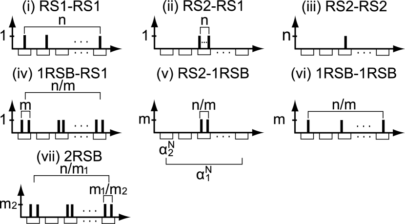
Figure 1: Possible saddle point for $\{q_{\nu}^{ab}\}$ at $K=2$. The horizontal axis represents the index of configurations running from 1 to $2^{N}$. All configurations are divided into $\alpha_{1}^{N}$-groups including $\alpha_{2}^{N}$-configurations. The vertical axis represents the number of ‘balls’.

1. RS1-RS1.

   There is no overlap between any of the configurations and

   $$(q_{1}^{ab},q_{2}^{ab})=(\delta_{ab},\delta_{ab}).$$ (20)

   Then, $S_{q}(q)$ and $\phi(n)$ are calculated as

   $$S_{q}(q)=\ln\left\{2^{N}(2^{N}-\alpha_{2}^{N})\cdots(2^{N}-(n-1)\alpha_{2}^{N})\right\}\sim Nn\ln 2,$$ (21)

   $$\phi(n)=n\left(\ln 2+\frac{\beta^{2}J^{2}}{4}\right).$$ (22)

   This is the standard ‘paramagnetic’ state of the REM. The free energy $f(T)=-\lim_{n\to 0}\phi(n)/\beta n$ and the thermodynamic entropy $s(T)=-\partial f(T)/\partial T$ per site $N$ can be calculated as

   $$f(T)=-T\ln 2-\frac{J^{2}}{4T},$$ (23)

   $$s(T)=\ln 2-\frac{J^{2}}{4T^{2}}.$$ (24)

2. RS2-RS1.

   In this case, there are overlaps at the first hierarchy and

   $$(q_{1}^{ab},q_{2}^{ab})=(1,\delta_{ab}).$$ (25)

   We obtain

   $$S_{q}(q)=N\left(\ln\alpha_{1}+n\ln\alpha_{2}\right),$$ (26)

   $$\phi(n)=\ln\alpha_{1}+\frac{\beta^{2}J^{2}}{4}n^{2}a_{1}+n\left(\ln\alpha_{2}+\frac{\beta^{2}J^{2}}{4}a_{2}\right).$$ (27)

   $\phi(n)$ is not proportional to $n$ and this solution is irrelevant at the limit of $n\to 0$.

3. RS2-RS2.

   All states have a same configuration and

   $$(q_{1}^{ab},q_{2}^{ab})=(1,1).$$ (28)

   We obtain

   $$S_{q}(q)=N\ln 2,$$ (29)

   $$\phi(n)=\ln 2+\frac{\beta^{2}J^{2}}{4}n^{2}.$$ (30)

   This is also an irrelevant solution at the limit of $n\to 0$.

4. 1RSB-RS1.

   The replica symmetry in the first hierarchy is broken by introducing an integer $m$ as

   $$(q_{1}^{ab},q_{2}^{ab})=(\delta_{m}(a,b),\delta_{ab}),$$ (31)

   where

   $$\delta_{m}(a,b)=\left\{\begin{array}[]{ll}1&\mbox{for}\ \lfloor(a-1)/m\rfloor=\lfloor(b-1)/m\rfloor\\ 0&\mbox{otherwise}\end{array}\right..$$ (34)

   Then, we have

   $$S_{q}(q)=Nn\left(\frac{1}{m}\ln\alpha_{1}+\ln\alpha_{2}\right),$$ (35)

   $$\phi(n;m)=n\left(\frac{1}{m}\ln\alpha_{1}+\frac{\beta^{2}J^{2}}{4}ma_{1}+\ln\alpha_{2}+\frac{\beta^{2}J^{2}}{4}a_{2}\right).$$ (36)

   $m$ is optimized so that $\phi(n)$ becomes maximum. We obtain a real value as $m=T/T_{1}$ and

   $$\phi(n)=n\left(\beta J\sqrt{a_{1}\ln\alpha_{1}}+\ln\alpha_{2}+\frac{\beta^{2}J^{2}}{4}a_{2}\right).$$ (37)

   Then, we have

   $$f(T)=-J\sqrt{a_{1}\ln\alpha_{1}}-T\ln\alpha_{2}-\frac{J^{2}}{4T}a_{2},$$ (38)

   $$s(T)=\ln\alpha_{2}-\frac{J^{2}}{4T^{2}}a_{2}.$$ (39)

5. RS2-1RSB.

   The replica symmetry in the second hierarchy is broken as

   $$(q_{1}^{ab},q_{2}^{ab})=(1,\delta_{m}(a,b)),$$ (40)

   $$S_{q}(q)=N\left(\ln\alpha_{1}+\frac{n}{m}\ln\alpha_{2}\right),$$ (41)

   $$\phi(n;m)=\ln\alpha_{1}+\frac{\beta^{2}J^{2}}{4}n^{2}a_{1}+n\left(\frac{1}{m}\ln\alpha_{2}+\frac{\beta^{2}J^{2}}{4}ma_{2}\right).$$ (42)

   We obtain $m=T/T_{2}$ and an irrelevant solution at $n\to 0$ as

   $$\phi(n)=\ln\alpha_{1}+\frac{\beta^{2}J^{2}}{4}n^{2}a_{1}+n\beta J\sqrt{a_{2}\ln\alpha_{2}}.$$ (43)

6. 1RSB-1RSB.

   The replica symmetry is broken in both the hierarchy levels as

   $$(q_{1}^{ab},q_{2}^{ab})=(\delta_{m}(a,b),\delta_{m}(a,b)),$$ (44)

   $$S_{q}(q)=N\frac{n}{m}\ln 2,$$ (45)

   $$\phi(n;m)=n\left(\frac{1}{m}\ln 2+\frac{\beta^{2}J^{2}}{4}m\right).$$ (46)

   Then, $m=T/T_{\rm c}$ and the result reduces to the standard 1RSB ‘spin-glass’ state of the REM as

   $$\phi(n)=n\beta J\sqrt{\ln 2},$$ (47)

   $$f(T)=-J\sqrt{\ln 2},$$ (48)

   $$s(T)=0.$$ (49)

7. 2RSB (two-step RSB).

   This solution is similar to the 1RSB-1RSB one but the parameters $m_{1}$ and $m_{2}$ take different values as

   $$(q_{1}^{ab},q_{2}^{ab})=(\delta_{m_{1}}(a,b),\delta_{m_{2}}(a,b)),$$ (50)

   $$S_{q}(q)=Nn\left(\frac{1}{m_{1}}\ln\alpha_{1}+\frac{1}{m_{2}}\ln\alpha_{2}\right),$$ (51)

   $$\phi(n;m_{1},m_{2})=n\left(\frac{1}{m_{1}}\ln\alpha_{1}+\frac{\beta^{2}J^{2}}{4}m_{1}a_{1}+\frac{1}{m_{2}}\ln\alpha_{2}+\frac{\beta^{2}J^{2}}{4}m_{2}a_{2}\right).$$

   (52)

   We obtain $m_{1}=T/T_{1}$, $m_{2}=T/T_{2}$ and

   $$\phi(n)=n\left(\beta J\sqrt{a_{1}\ln\alpha_{1}}+\beta J\sqrt{a_{2}\ln\alpha_{2}}\right),$$ (53)

   $$f(T)=-J\sqrt{a_{1}\ln\alpha_{1}}-J\sqrt{a_{2}\ln\alpha_{2}},$$ (54)

   $$s(T)=0.$$ (55)

As we mentioned above, the solutions (ii), (iii) and (v) are irrelevant for constructing the free energy, since they do not give correct behavior of $\phi(n)$ at the limit $n\to 0$. From the other solutions, we should choose a suitable solution by considering the physical plausibility, which leads to two situations depending on the hierarchy parameters.

The first situation is the case $T_{2}<T_{1}$. In this case, two phase transitions, reflecting the entropy crises in each hierarchy, occur as temperature decreases. At high temperatures, the correct solution is given by RS1-RS1 solution (i) being the usual paramagnetic one. As temperature decreases, at $T=T_{1}$ a phase transition occurs and the system goes to the 1RSB-RS1 phase (iv). To understand this transition, we should identify the entropies of each hierarchy $s_{\nu}(T)$ ($\nu=1,2$) which are given by

$$s_{\nu}(T)=\ln\alpha_{\nu}-\frac{J^{2}}{4T}a_{\nu}.$$ (56)

The total entropy $s(T)$ is reproduced by the summation of the ones in each hierarchy as $s(T)=\sum_{\nu}s_{\nu}(T)$. At $T=T_{1}$, the entropy of the first hierarchy becomes zero and the system is partially frozen to its ground state in the first hierarchy, which can be clearly seen in the solution (iv). Similarly, at $T=T_{2}<T_{1}$, the entropy of the second hierarchy also becomes zero, which leads to a phase transition from (iv) to the 2RSB solution (vii). The above RSB transitions are hence interpreted as the entropy crises in different hierarchies, which sequentially occurs from the upper macroscopic to lower microscopic levels of hierarchy.

The other case is for $T_{1}\leq T_{2}$. In this case, the correct solution is given by (i) for $T>T_{\rm c}$ and by (vi) for $T\leq T_{\rm c}(<T_{2})$. This can be easily found since a possible branch at low temperatures, which should continuously connect to the high temperature solution (i), is only (iv) in this case. This solution indicates that the hierarchical structure becomes irrelevant and the standard REM result is reproduced.

The solution for the case $T_{1}\leq T_{2}$ might give a question to the hierarchical entropy $s_{\nu}$ since the second-hierarchy entropy $s_{2}(T)$ becomes negative in the region $T_{\rm c}<T<T_{2}$. This implies that $s_{\nu}(T)$ has its physical significance only in the case that the entropies in upper levels of hierarchy $s_{\mu}(T)$ with $\mu<\nu$ vanish. This point requires further discussions and is revisited in section 4.

Now, we summarize the behavior of thermodynamic functions as follows. The schematic behaviors of the entropy and the free energy are also depicted in figures 3 and 3, respectively.

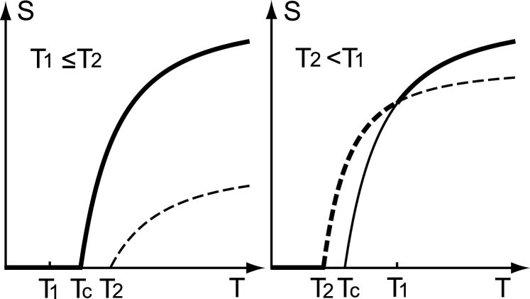
Figure 2: The entropy $s(T)$ of the GREM at $K=2$. The dashed line represents the entropy of the second hierarchy and the solid line the total entropy. The actual entropy takes the bold parts.

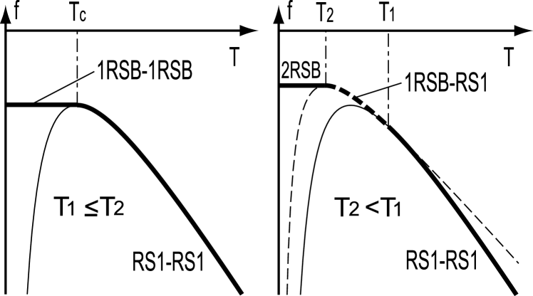
Figure 3: The free energy $f(T)$ of the GREM at $K=2$. From among several curves representing possible phases, the actual free energy takes the bold parts.

• $T_{2}<T_{1}$

  $$s(T)=\left\{\begin{array}[]{ll}\ln 2-\frac{J^{2}}{4T^{2}}&T_{1}\leq T\\ \ln\alpha_{2}-\frac{J^{2}}{4T^{2}}a_{2}&T_{2}\leq T\leq T_{1}\\ 0&T\leq T_{2}\end{array}\right.,$$ (60)

  $$f(T)=\left\{\begin{array}[]{ll}-T\ln 2-\frac{J^{2}}{4T}&T_{1}\leq T\\ -J\sqrt{a_{1}\ln\alpha_{1}}-T\ln\alpha_{2}-\frac{J^{2}}{4T}a_{2}&T_{2}\leq T\leq T_{1}\\ -J\left(\sqrt{a_{1}\ln\alpha_{1}}+\sqrt{a_{1}\ln\alpha_{1}}\right)&T\leq T_{2}\end{array}\right..$$ (64)

• $T_{1}\leq T_{2}$

  $$s(T)=\left\{\begin{array}[]{ll}\ln 2-\frac{J^{2}}{4T^{2}}&T_{\rm c}\leq T\\ 0&T\leq T_{\rm c}\end{array}\right.,$$ (67)

  $$f(T)=\left\{\begin{array}[]{ll}-T\ln 2-\frac{J^{2}}{4T}&T_{\rm c}\leq T\\ -J\sqrt{\ln 2}&T\leq T_{\rm c}\end{array}\right..$$ (70)

This result coincides with the original one by the microcanonical ensemble formalism [23]. As we see, the phase at lower temperature is described by the 2RSB for a suitable choice of the hierarchy parameters. The generalization of the discussion to $K\geq 3$ is straightforward, where the higher step RSB is realized at lower temperature region.

3 The GREM: (2) spin representation

Our main motivation for introducing the GREM is to understand spin-glass phase transitions characterized by the higher step RSB. However, the GREM in the previous section is defined by randomly distributed energy, and the relation of the GREM with other random models expressed by spins is not clear. On the other hand, the standard REM is known as the limit $p\to\infty$ of the $p$-body interacting spin-glass model. This observation is very useful to find a connection between the REM with the 1RSB and the SK model with the full-step RSB. Therefore, it is natural to ask whether one can construct a spin-glass model which includes the GREM as a limit. In this section, we propose a hierarchical $p$-body interacting spin-glass model and demonstrate that this yields the same thermodynamic behavior as the GREM at the limit $p\to\infty$.

3.1 Hierarchical $p$-body interacting spin-glass model

We define the Hamiltonian

$$H=-\sum_{\nu=1}^{K}\sum_{(i_{1}\cdots i_{p})}^{N_{\nu}}J_{i_{1}\cdots i_{p}}^{(\nu)}\sigma_{i_{1}}\cdots\sigma_{i_{p}},$$ (71)

where $\sigma_{i}$ is the Ising spin on site $i$. In the $\nu$th hierarchy, the sum is taken over possible combinations of $N_{\nu}$-spins, where $N_{\nu}$ is given by $2^{N_{\nu}}=M_{\nu}$ and $M_{\nu}$ is in (1). Due to the properties (1) and (2), $N_{1}<N_{2}<\cdots<N_{K}=N$. The random interaction $J_{i_{1}\cdots i_{p}}^{(\nu)}$ distributes in Gaussian with the variance

$$[(J_{i_{1}\cdots i_{p}}^{(\nu)})^{2}]=\frac{NJ^{2}}{2}a_{\nu}\frac{p!}{N_{\nu}^{p}},$$ (72)

where $a_{\nu}$ satisfies (5).

3.2 Energy-level distributions

Before calculating the thermodynamic functions, we examine the energy-level distribution functions. For a given configuration $\{\sigma_{i}\}$, the single-level distribution is calculated as

$$\left[\delta\left(E-H(\{\sigma_{i}\})\right)\right] = \int\frac{dt}{2\pi}e^{itE}\left[\exp\left(it\sum_{\nu=1}^{K}\sum_{(i_{1}\cdots i_{p})}^{N_{\nu}}J_{i_{1}\cdots i_{p}}^{(\nu)}\sigma_{i_{1}}\cdots\sigma_{i_{p}}\right)\right]$$ (73)

$$= \frac{1}{\sqrt{\pi NJ^{2}}}\exp\left(-\frac{E^{2}}{NJ^{2}}\right).$$

Thus, the single energy-level distribution is equivalent to the REM/GREM. In the same way, the two-point correlation for configurations $\{\sigma_{i}^{1}\}$ and $\{\sigma_{i}^{2}\}$ is calculated as

$$\left[\delta\left(E-H(\{\sigma_{i}^{1}\})\right)\delta\left(E^{\prime}-H(\{\sigma_{i}^{2}\})\right)\right]$$ (74)

$$= \frac{1}{\pi NJ^{2}\sqrt{1-v^{2}}}\exp\left\{-\frac{(E+E^{\prime})^{2}}{2NJ^{2}(1+v)}-\frac{(E-E^{\prime})^{2}}{2NJ^{2}(1-v)}\right\},$$

where

$$v=\sum_{\nu=1}^{K}a_{\nu}(q_{\nu}^{12})^{p},$$ (75)

$$(q_{\nu}^{12})^{p}=\frac{p!}{N_{\nu}^{p}}\sum_{(i_{1}\cdots i_{p})}\sigma_{i_{1}}^{1}\sigma_{i_{1}}^{2}\cdots\sigma_{i_{p}}^{1}\sigma_{i_{p}}^{2}\sim\left(\frac{1}{N_{\nu}}\sum_{i=1}^{N_{\nu}}\sigma_{i}^{1}\sigma_{i}^{2}\right)^{p}.$$ (76)

This form is the same as that of the GREM [23]. The quantity $v$ depends on the spin configurations and it goes to the result of the GREM at the limit $p\to\infty$.

3.3 Replica method

We calculate the ensemble average of the $n$th power of the partition function. Introducing the replica indices $a=1,2,\cdots,n$, we obtain

$$[Z^{n}] = \left[\Tr\exp\left\{\sum_{\nu=1}^{K}\sum_{(i_{1}\cdots i_{p})}^{N_{\nu}}\beta J_{i_{1}\cdots i_{p}}^{(\nu)}\sum_{a=1}^{n}\sigma_{i_{1}}^{a}\cdots\sigma_{i_{p}}^{a}\right\}\right]$$ (77)

$$= \Tr\exp\left\{\frac{N\beta^{2}J^{2}}{2}\sum_{\nu=1}^{K}a_{\nu}\sum_{a>b}^{n}\left(\frac{1}{N_{\nu}}\sum_{i=1}^{N_{\nu}}\sigma_{i}^{a}\sigma_{i}^{b}\right)^{p}+\frac{Nn\beta^{2}J^{2}}{4}\right\}.$$

The order parameters $q_{\nu}^{ab}\sim\sum_{i=1}^{N_{\nu}}\sigma_{i}^{a}\sigma_{i}^{b}/N_{\nu}$ and auxiliary variables $\tilde{q}_{\nu}^{ab}$ are introduced following the standard prescription as

$$[Z^{n}] = \int dq_{\nu}^{ab}\Tr\prod_{\nu=1}^{K}\prod_{a>b}^{n}\delta\left(q_{\nu}^{ab}-\frac{1}{N_{\nu}}\sum_{i=1}^{N_{\nu}}\sigma_{i}^{a}\sigma_{i}^{b}\right)$$ (78)

$$\times\exp\left\{\frac{N\beta^{2}J^{2}}{2}\sum_{\nu=1}^{K}a_{\nu}\sum_{a>b}^{n}\left(q_{\nu}^{ab}\right)^{p}+\frac{Nn\beta^{2}J^{2}}{4}\right\}$$

$$= \int dq_{\nu}^{ab}d\tilde{q}_{\nu}^{ab}\Tr\exp\left\{-N\beta^{2}J^{2}\sum_{\nu=1}^{K}a_{\nu}\sum_{a>b}^{n}\tilde{q}_{\nu}^{ab}\left(q_{\nu}^{ab}-\frac{1}{N_{\nu}}\sum_{i=1}^{N_{\nu}}\sigma_{i}^{a}\sigma_{i}^{b}\right)\right.$$

$$\left.+\frac{N\beta^{2}J^{2}}{2}\sum_{\nu=1}^{K}a_{\nu}\sum_{a>b}^{n}\left(q_{\nu}^{ab}\right)^{p}+\frac{Nn\beta^{2}J^{2}}{4}\right\}.$$

The integrations are evaluated by the saddle-point method. Using the saddle point to be obtained, we can write

$$[Z^{n}] = \exp\left\{-\frac{N\beta^{2}J^{2}}{2}(p-1)\sum_{\nu=1}^{K}a_{\nu}\sum_{a>b}^{n}(q_{\nu}^{ab})^{p}+\frac{Nn\beta^{2}J^{2}}{4}\right.$$ (79)

$$\left.+\ln\Tr\exp\left(N\beta^{2}J^{2}\sum_{\nu=1}^{K}\frac{a_{\nu}}{N_{\nu}}\sum_{a>b}^{n}\tilde{q}_{\nu}^{ab}\sum_{i=1}^{N_{\nu}}\sigma_{i}^{a}\sigma_{i}^{b}\right)\right\},$$

where

$$\tilde{q}_{\nu}^{ab}=\frac{p}{2}(q_{\nu}^{ab})^{p-1}.$$ (80)

In the following calculation, we set $K=2$ for simplicity. Then, the partition function reads

$$[Z^{n}] = \exp\left\{-\frac{N\beta^{2}J^{2}}{2}(p-1)\sum_{\nu=1}^{2}a_{\nu}\sum_{a>b}^{n}(q_{\nu}^{ab})^{p}+\frac{Nn\beta^{2}J^{2}}{4}\right.$$ (81)

$$+N_{1}\ln\Tr\exp\left(N\beta^{2}J^{2}\sum_{\nu=1}^{2}\frac{a_{\nu}}{N_{\nu}}\sum_{a>b}^{n}\tilde{q}_{\nu}^{ab}\sigma^{a}\sigma^{b}\right)$$

$$\left.+(N-N_{1})\ln\Tr\exp\left(N\beta^{2}J^{2}\frac{a_{2}}{N}\sum_{a>b}^{n}\tilde{q}_{2}^{ab}\sigma^{a}\sigma^{b}\right)\right\},$$

and the saddle-point equation can be derived as

$$q_{1}^{ab}=\frac{\Tr\sigma^{a}\sigma^{b}\exp\left(N\beta^{2}J^{2}\sum_{\nu=1}^{2}\frac{a_{\nu}}{N_{\nu}}\sum_{a>b}^{n}\tilde{q}_{\nu}^{ab}\sigma^{a}\sigma^{b}\right)}{\Tr\exp\left(N\beta^{2}J^{2}\sum_{\nu=1}^{2}\frac{a_{\nu}}{N_{\nu}}\sum_{a>b}^{n}\tilde{q}_{\nu}^{ab}\sigma^{a}\sigma^{b}\right)},$$ (82)

$$q_{2}^{ab}=\frac{N_{1}}{N}q_{1}^{ab}+\frac{N-N_{1}}{N}\frac{\Tr\sigma^{a}\sigma^{b}\exp\left(\beta^{2}J^{2}a_{2}\sum_{a>b}^{n}\tilde{q}_{2}^{ab}\sigma^{a}\sigma^{b}\right)}{\Tr\exp\left(\beta^{2}J^{2}a_{2}\sum_{a>b}^{n}\tilde{q}_{2}^{ab}\sigma^{a}\sigma^{b}\right)}.$$ (83)

The saddle-point equations can be easily solved at $p=\infty$ since the possible solutions of $\tilde{q}^{ab}_{1,2}$ are restricted to 0 or $\infty$. We can repeat the similar discussion as that of the previous section. For example, the RS1-RS1 solution $(q_{1}^{ab},q_{2}^{ab})=(\delta_{ab},\delta_{ab})$ gives the same result (22). In A, we study the 1RSB-RS1 and the 2RSB solutions as nontrivial cases. All cases give the same result as that of the previous section, which shows that the present hierarchical spin model at $p\to\infty$ is equivalent to the GREM.

Here, we must mention a similarity between our model and the diluted generalized random energy model proposed by Saakian in [25]. Although the hierarchical structure is the same for both the models, the form of the Hamiltonian is slightly different. In addition, he has not shown explicitly that his model is equivalent to the GREM. In principle, it might be possible to define several hierarchical spin models which reduce to the GREM at a certain limit. We consider that our model is the simplest one among such models.

We also see that our model is very different from other spin models with the higher step RSB such as the SK model. Each spin is not treated in an equivalent manner, which is clearly the origin of the hierarchical ordering. As a random spin model with a hierarchy, similar models on a hierarchical lattice are proposed in [30, 31]. These models are shown to be useful to study RSB solutions. The advantage of our model is that it can be treated by the mean-field theory and that the analytical result is available. We further discuss this point by considering similar hierarchical models in section 5.

4 Generalization of complexity

As we see, it is shown that lower temperature phases in the GREM are described by the higher step RSB. Here, to investigate such systems in detail, we generalize the assessment scheme of complexity for higher step RSB systems. To this end, we start from a brief review of how the concept of complexity is introduced.

The concept of complexity is closely related to the multi-valley structure of the phase space. In a number of systems with quenched randomness such as spin glasses, the phase space is considered to be divided into exponentially many disjoint sets in the thermodynamic limit [32, 33]. Each component of the disjoint sets is sometimes called pure state and is schematically described by a valley in the phase space. Each pure state labeled by $\gamma$ has its own free energy value $f_{\gamma}$. The number of pure states having the free energy value $f$, $\mathcal{N}(f)$, is scaled as

$$\mathcal{N}(f)\sim e^{N\Sigma(f)},$$ (84)

where the exponent $\Sigma(f)\sim O(1)$ is called complexity. Note that an inequality $\Sigma(f)\geq 0$ holds since complexity is the logarithm of the number of states. The partition function of the whole system is written by the summation of the weight of each pure state $\gamma$ as $Z=\sum_{\gamma}Z_{\gamma}=\sum_{\gamma}e^{-N\beta f_{\gamma}}$. This total partition function can also be written by using complexity as

$$Z\sim\int dfe^{N\left(-\beta f+\Sigma(f)\right)}.$$ (85)

The saddle-point method yields the equilibrium free energy $f_{\rm eq}=-(1/N\beta)\ln Z$ as

$$-\beta f_{\rm eq}=\max_{f_{-}\leq f\leq f_{+}}\left\{-\beta f+\Sigma(f)\right\}.$$ (86)

The inequality $\Sigma(f)\geq 0$ leads to the upper and lower bounds of $f$, $f_{+}$ and $f_{-}$, respectively. Equation (86) means that complexity of the system is necessary to obtain the equilibrium free energy. This is quite general; however, the actual evaluation scheme of complexity depends on the number of RSB steps.

4.1 The 1RSB case

To evaluate complexity, we need some information about the phase-space structure of the system. In the 1RSB case, it is considered that the phase space has many valleys corresponding to pure states. However, its structure is not complicated because all the pure states are statistically equivalent and any meta-structure is not present in the phase space (see figure 5). In such a situation, it is natural to characterize the phase-space structure by two typical overlaps: the one in single pure state $q_{1}$ and the other one between pure states $q_{0}$. These are nothing but the 1RSB spin-glass-order parameters. This implies that the 1RSB free energy $f_{\rm 1RSB}(m)$ parameterized by the breaking parameter $m$ has some information about the phase space. Actually, according to Monasson’s argument [11], the 1RSB free energy is proportional to a generating function of complexity $g(x)$ as $f_{\rm 1RSB}(m=x)=-g(x)/\beta x$. The definition of $g(x)$ is given by

$$g(x)=\frac{1}{N}\ln\left(\sum_{\gamma}(Z_{\gamma})^{x}\right)=\max_{f_{-}\leq f\leq f_{+}}\left\{-\beta xf+\Sigma(f)\right\}.$$ (87)

Using this equation, we can calculate complexity by Legendre transformation

$$\Sigma(f)=\min_{x}\left\{g(x)+\beta xf\right\}.$$ (88)

If the complexity is convex and analytic, we can express the pure-state free energy and complexity in parameterized forms as

$$-\beta f(x)=\frac{\partial g}{\partial x},$$ (89)

$$\Sigma(x)=g(x)-x\frac{\partial g}{\partial x}.$$ (90)

Once we obtain complexity $\Sigma(f)$ from $g(x)$ by (88), the equilibrium free energy can be calculated by (86). These procedures constitute the scheme of how to assess complexity and equilibrium free energy in the 1RSB level.

Before proceeding to the 2RSB case, we mention the equivalence between the generating function $g(x)$ and the 1RSB free energy $f_{\rm 1RSB}(m)$. We can expect the self-averaging property of the generating function $g(x)$, which is defined by (87) and intrinsically depends on the quenched randomness. Hence, the typical generating function $g(x)$ can be replaced by the averaged one. This consideration, in conjunction with the replica method, yields

$$g(x)=\frac{1}{N}\left[\ln\left(\sum_{\gamma}(Z_{\gamma})^{x}\right)\right]=\lim_{y\to 0}\frac{\partial}{\partial y}\frac{1}{N}\ln\left[\left(\sum_{\gamma}(Z_{\gamma})^{x}\right)^{y}\right].$$ (91)

Although exact evaluation of the right-hand side of (91) is difficult, we can derive the following expression for integer $x$ and $y$:

$$\left[\left(\sum_{\gamma}(Z_{\gamma})^{x}\right)^{y}\right] = \left[\left\{\sum_{\gamma}\left(\sum_{\{\sigma\}}e^{-\beta H(\{\sigma\})}\theta_{\gamma}(\{\sigma\})\right)^{x}\right\}^{y}\right]$$

$$= \left[\prod_{\mu=1}^{y}\sum_{\gamma_{\mu}}\prod_{\nu=1}^{x}\sum_{\{\sigma_{\nu}^{\mu}\}}\exp\left(-\beta\sum_{\mu=1}^{y}\sum_{\nu=1}^{x}H(\{\sigma_{\nu}^{\mu}\})\right)\Theta(x,y)\right],$$

where $\{\sigma\}$ denotes the dynamical variables (spins) and $\theta_{\gamma}(\{\sigma\})$ is the indicator function such that $\theta_{\gamma}(\{\sigma\})=1$ if $\{\sigma\}\in\gamma$, and 0 otherwise. We also define

$$\Theta(x,y)=\prod_{\mu=1}^{y}\prod_{\nu=1}^{x}\theta_{\gamma_{\mu}}(\{\sigma_{\nu}^{\mu}\}).$$ (93)

For the evaluation of (LABEL:phi), the following observations are important.

• The summation is taken over all possible configurations of $xy$ replica spins.

• However, the factor $\Theta(x,y)$ allows only contributions from configurations in which $xy$ replicas are equally assigned to $y$ pure states with the weight $x$.

These points describe nothing more than the physical picture of the 1RSB phase, in which case we evaluate $[Z^{n}]$ with substitution of $n=xy$ and $m=x$. Hence, we obtain

$$g(x)=\lim_{y\to 0}\frac{\partial}{\partial y}\phi_{\rm 1RSB}(n=yx,m=x)=-\beta xf_{\rm 1RSB}(x),$$ (94)

where $\phi_{\rm 1RSB}(n,m)$ is $(1/N)\ln[Z^{n}]$ assessed under the 1RSB ansatz with the breaking parameter $m$.

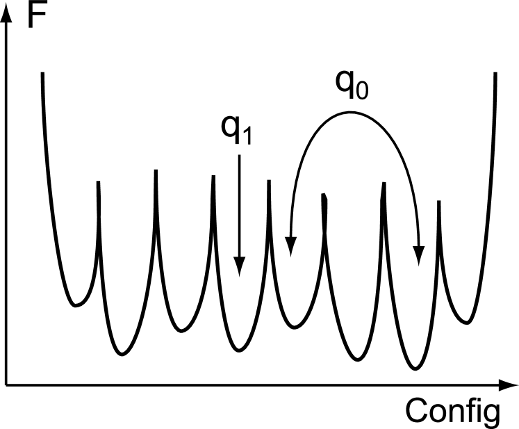
Figure 4: Schematic picture of the phase space in the 1RSB phase. The vertical axis represents the free energy and the horizontal one schematically describes the configuration space of dynamical variables. Each valley corresponds to a pure state. There is no meta-structure constituted by pure states.

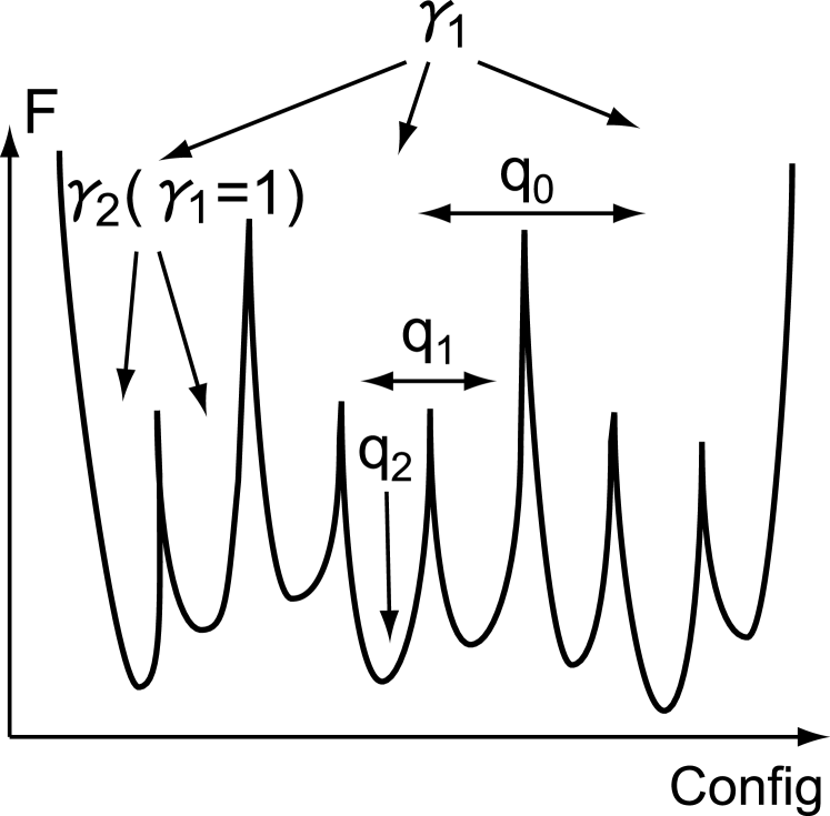
Figure 5: Schematic picture of the phase space in the 2RSB phase. Some valleys constitute a large ‘valley’ in a more macroscopic level. Three overlap parameters are necessary to characterize this phase-space structure.

4.2 The 2RSB case

Next we consider the 2RSB case. From the physical picture supposed in the 2RSB, the phase space structure can be schematically depicted as figure 5. There are two macroscopically distinct levels of hierarchies. We here call them hierarchies 1 and 2 . Hierarchy 2 is constituted by pure states labeled by $\gamma_{2}$. On the other hand, the hierarchy 1 is the one in a coarse-grained level. Each coarse-grained state in this level, labeled by $\gamma_{1}$, is constituted by a group of pure states. The phase space is characterized by three overlaps: $q_{2}$ in a single pure state, $q_{1}$ between two pure states in the same state of hierarchy 1 and $q_{0}$ between different states in hierarchy 1.

Let us accept and employ the above description to obtain complexity in the 2RSB level. This description enables us to express the partition function as

$$Z=\sum_{\gamma_{1}}\left(\sum_{\gamma_{2}(\gamma_{1})}Z_{\gamma_{2}(\gamma_{1})}\right),$$ (95)

where $\gamma_{1}$ specifies coarse-grained states in hierarchy 1 and $\gamma_{2}(\gamma_{1})$ represents a pure state in a large valley $\gamma_{1}$. Similarly to the 1RSB case, we can introduce a generating function $g_{1}(x_{1},x_{2})$ as

$$g_{1}(x_{1},x_{2})=\frac{1}{N}\ln\left\{\sum_{\gamma_{1}}\left(\sum_{\gamma_{2}(\gamma_{1})}(Z_{\gamma_{2}(\gamma_{1})})^{x_{2}}\right)^{x_{1}}\right\}.$$ (96)

Actually, this generating function $g_{1}(x_{1},x_{2})$ corresponds to the 2RSB free energy with the breaking parameters $m_{1}$ and $m_{2}$ as

$$f_{\rm 2RSB}(m_{1}=x_{1}x_{2},m_{2}=x_{2})=-\frac{1}{\beta x_{1}x_{2}}g_{1}(x_{1},x_{2}).$$ (97)

This correspondence can be understood by following a discussion being similar to that in the previous 1RSB case.

The next task is to construct a procedure to obtain complexity from $g_{1}(x_{1},x_{2})$. The following expression of $g_{1}(x_{1},x_{2})$ is useful for this purpose:

$$e^{Ng_{1}(x_{1},x_{2})} = \sum_{\gamma_{1}}\left(\sum_{\gamma_{2}(\gamma_{1})}(Z_{\gamma_{2}(\gamma_{1})})^{x_{2}}\right)^{x_{1}}$$ (98)

$$= \sum_{\gamma_{1}}\left(\int dfe^{N(-\beta x_{2}f+\widehat{\Sigma}_{2}(f|\gamma_{1}))}\right)^{x_{1}}$$

$$= \int df_{1}e^{N(x_{1}f_{1}+\Sigma_{1}(f_{1}|x_{2}))},$$

where we introduce two entropy-like quantities $\Sigma_{1}(f_{1}|x_{2})$ and $\widehat{\Sigma}_{2}(f|\gamma_{1})$, and another generating function $f_{1}(x_{2}|\gamma_{1})$ defined in a large valley $\gamma_{1}$ as

$$f_{1}(x_{2}|\gamma_{1})=\frac{1}{N}\ln\left(\sum_{\gamma_{2}(\gamma_{1})}(Z_{\gamma_{2}(\gamma_{1})})^{x_{2}}\right)=\max_{f_{-}\leq f\leq f_{+}}\left\{-\beta x_{2}f+\widehat{\Sigma}_{2}(f|\gamma_{1})\right\}.$$ (99)

The physical meanings of these quantities are as follows. The quantity $\widehat{\Sigma}_{2}(f|\gamma_{1})$ is the complexity in a large valley $\gamma_{1}$, i.e. it characterizes the number of pure states having free energy value $f$ in a valley $\gamma_{1}$. The generating function $f_{1}(x_{2}|\gamma_{1})$ plays a role of a coarse-grained free energy in a valley $\gamma_{1}$. Then, in the hierarchy 1, the number of valleys having ‘free energy’ value $f_{1}(x_{2}|\gamma_{1})=f_{1}$, $\mathcal{N}_{1}(f_{1}|x_{2})$, is also important. This quantity $\mathcal{N}_{1}$ intrinsically depends on $x_{2}$ and is characterized by the exponent $\Sigma_{1}(f_{1}|x_{2})$ as $\mathcal{N}_{1}(f_{1}|x_{2})=\exp\{N\Sigma_{1}(f_{1}|x_{2})\}$. In this sense, $\Sigma_{1}(f_{1}|x_{2})$ is the ‘complexity of hierarchy 1’. According to (98), we can see that $g_{1}(x_{1},x_{2})$ and $\Sigma_{1}(f_{1}|x_{2})$ are related with each other by the Legendre transformation

$$g_{1}(x_{1},x_{2})=\max_{f_{1-}\leq f_{1}\leq f_{1+}}\left\{x_{1}f_{1}+\Sigma_{1}(f_{1}|x_{2})\right\}.$$ (100)

The bounds of values of $f_{1}$ are determined by the constraint $\Sigma_{1}(f_{1}|x_{2})\geq 0$. Hence, we can calculate the first-hierarchy complexity $\Sigma_{1}(f_{1}|x_{2})$ by

$$\Sigma_{1}(f_{1}|x_{2})=\min_{x_{1}}\left\{g_{1}(x_{1},x_{2})-x_{1}f_{1}\right\}.$$ (101)

Using $\Sigma_{1}(f_{1}|x_{2})$, we can construct the generating function of the original complexity $\Sigma(f)$, $g_{2}(x_{2})$, which is obtained by

$$g_{2}(x_{2})=\max_{f_{1-}\leq f_{1}\leq f_{1+}}\left\{f_{1}+\Sigma_{1}(f_{1}|x_{2})\right\}.$$ (102)

There are two noteworthy points concerning this equation. First, the expression of $g_{2}(x_{2})$ is apparently the same as $g_{1}(1,x_{2})$. However, there is one difference we should notice in the evaluation of first-hierarchy complexity $\Sigma_{1}(f_{1}|x_{2})$: we should carefully deal with $g_{1}(x_{1},x_{2})$ derived from the 2RSB solution (see (97)) since it includes inappropriate branches which lead to negative $\Sigma_{1}(f_{1}|x_{2})$. The basic line of the above procedures using (101) and (102) is correct even with such a difference. This point will be clearer when we apply the complexity analysis to the GREM in section 4.3. The second point is the reason why $g_{2}(x_{2})$ becomes the generating function of complexity. This can be understood by putting $x_{1}=1$ in (96). In the case of $x_{1}=1$, the discrimination of hierarchies 1 and 2 vanishes and the summation runs over all pure states equally, which elucidates the fact that $g_{2}(x_{2})$ is indeed the generating function of complexity.

Once we get $g_{2}(x_{2})$, complexity $\Sigma(f)$ can be assessed in the same way as the 1RSB case:

$$\Sigma(f)=\min_{x_{2}}\left\{\beta x_{2}f+g_{2}(x_{2})\right\}.$$ (103)

This completes procedures for evaluating complexity $\Sigma(f)$. The equilibrium free energy is again evaluated from $\Sigma(f)$ by (86).

We here summarize the procedures to obtain complexity in the 2RSB level.

1. Calculate the 2RSB solution $f_{\rm 2RSB}(m_{1},m_{2})$ and introduce the generating function $g_{1}(x_{1},x_{2})$ by (97).

2. Calculate the first-hierarchy complexity $\Sigma_{1}(f_{1}|x_{2})$ by (101).

3. Calculate the generating function of complexity $g_{2}(x_{2})$ by (102).

4. Calculate complexity $\Sigma(f)$ by (103).

Note that quantities depending on states, such as $f_{1}(x_{2}|\gamma_{1})$ and $\widehat{\Sigma}_{2}(x_{2}|\gamma_{1})$, do not appear explicitly in these procedures. It is natural since those quantities cannot be calculated from the averaged quantities.

The procedures investigated in this subsection can be generalized to the $k$-step RSB with arbitrary $k$. In such a case, we should introduce the $i$th hierarchy complexity $\Sigma_{i}$ for $1\leq i\leq k$. We start from the $k$-step RSB solution being the first generating function $g_{1}$. The $i$th complexity $\Sigma_{i}$ is derived from $g_{i}$ as (101) and the $(i+1)$st generating function $g_{i+1}$ is calculated from $\Sigma_{i}$ as (102). These procedures are continued from $i=1$ to $k$, and the $k$th complexity corresponds to the original complexity $\Sigma(f)$. The Parisi’s breaking parameters $\{m_{i}\}$ are generally related to the parameters controlling the $i$th complexity, $\{x_{i}\}$, as $x_{i}=m_{i}/m_{i+1}$ with $x_{k}=m_{k}$.

4.3 Application to the GREM

We saw in sections 2 and 3 that the GREM with $K=2$ can be described by the 2RSB ansatz. Hence, the 2RSB formulation of complexity can be applied straightforwardly.

According to (52) and (97), the generating function of the GREM is given by

$$g_{1}(x_{1},x_{2})=\ln\alpha_{1}+\frac{\beta^{2}J^{2}}{4}a_{1}x_{1}^{2}x_{2}^{2}+x_{1}\left(\ln\alpha_{2}+\frac{\beta^{2}J^{2}}{4}a_{2}x_{2}^{2}\right).$$ (104)

The first-hierarchy complexity $\Sigma_{1}(f_{1}|x_{2})$ is then calculated from (101) as

$$\Sigma_{1}(f_{1}|x_{2})=\ln\alpha_{1}-\frac{1}{\beta^{2}J^{2}a_{1}x_{2}^{2}}\left\{f_{1}-\left(\ln\alpha_{2}+\frac{\beta^{2}J^{2}}{4}a_{2}x_{2}^{2}\right)\right\}^{2}.$$ (105)

For this calculation, the following $x_{1}$-parameterized forms, which are valid if $\Sigma_{1}$ is convex and analytic, are quite useful:

$$f_{1}(x_{1}|x_{2})=\frac{\partial g_{1}}{\partial x_{1}},$$ (106)

$$\Sigma_{1}(x_{1}|x_{2})=g_{1}(x_{1},x_{2})-x_{1}f_{1}(x_{1}|x_{2}).$$ (107)

By the constraint $\Sigma_{1}(f_{1}|x_{2})\geq 0$, we find the possible range of $f_{1}$:

$$\left|f_{1}-\left(\ln\alpha_{2}+\frac{\beta^{2}J^{2}}{4}a_{2}x_{2}^{2}\right)\right|\leq\beta Jx_{2}\sqrt{a_{1}\ln\alpha_{1}}.$$ (108)

Equation (102) gives the generating function of complexity

$$g_{2}(x_{2})=\max_{f_{1-}\leq f_{1}\leq f_{1+}}\left\{f_{1}+\ln\alpha_{1}-\frac{\left\{f_{1}-\left(\ln\alpha_{2}+\frac{\beta^{2}J^{2}}{4}a_{2}x_{2}^{2}\right)\right\}^{2}}{\beta^{2}J^{2}a_{1}x_{2}^{2}}\right\}.$$ (109)

The behavior of $g_{2}(x_{2})$ changes depending on the hierarchy parameters.

For the case $T_{2}<T_{1}$, we have

$$g_{2}(x_{2})=\left\{\begin{array}[]{ll}\ln 2+\frac{\beta^{2}J^{2}}{4}x_{2}^{2}&0\leq x_{2}\leq\frac{\beta_{1}}{\beta}\\ \ln\alpha_{2}+\frac{\beta^{2}J^{2}}{4}a_{2}x_{2}^{2}+\beta Jx_{2}\sqrt{a_{1}\ln\alpha_{1}}&\frac{\beta_{1}}{\beta}\leq x_{2}\end{array}\right..$$ (112)

Clearly, $g_{2}(x_{2})$ is the same as $g_{1}(1,x_{2})$ in (104) for small $x_{2}$ but different for large $x_{2}$. This is because for large $x_{2}$ the maximizer in (109) should be fixed to the point $f_{1+}$ where $\Sigma_{1}(f_{1+}|x_{2})=0$, but such a freezing effect in hierarchy 1 is not reflected in (104). This leads to an inappropriate branch of $g_{1}(1,x_{2})$.

The complexity corresponding to (112) is assessed by (6) as

$$\Sigma(f)=\left\{\begin{array}[]{ll}\ln 2-(f/J)^{2}&f_{\rm c1}\leq f\leq 0\\ \ln\alpha_{2}-\frac{1}{a_{2}}(f/J+\sqrt{a_{1}\ln\alpha_{1}})^{2}&f_{\rm c2}\leq f\leq f_{\rm c1}\end{array}\right.,$$ (115)

where $f_{\rm c1}=-J\sqrt{\ln\alpha_{1}/a_{1}}$ and $f_{\rm c2}=-J(\sqrt{a_{1}\ln\alpha_{1}}+\sqrt{a_{2}\ln\alpha_{2}})$. The lower bound $f_{\rm c2}$ yields the vanishing point of complexity as $\Sigma(f_{\rm c2})=0$. This reproduces (64) as the equilibrium free energy.

For the case $T_{1}\leq T_{2}$, we also have (112) from (102), but the large-$x_{2}$ branch of the function is inappropriate. This becomes clear by calculating the resultant complexity

$$\Sigma(f)=\ln 2-\left(\frac{f}{J}\right)^{2},$$ (116)

for $f_{\rm c}=-J\sqrt{\ln 2}\leq f\leq 0$, where $f_{\rm c}$ is the vanishing point of complexity $\Sigma(f_{\rm c})=0$. The inequality $f_{\rm c1}<f_{\rm c}$ means the irrelevance of the large-$x_{2}$ branch of $g_{2}(x_{2})$. This result rederives the standard REM result (70), which can be derived by the 1RSB ansatz, as the equilibrium free energy. Hence, all the results for the GREM are correctly reproduced by the complexity analysis.

Comparing the results (115) and (116), we can find that the 1RSB ansatz gives the correct result for small $|f|$ even in the case $T_{2}<T_{1}$. This means that the 2RSB solution gives the same result as the 1RSB one as long as the first-hierarchy complexity is positive, i.e. the maximizer in (109) is given by a value $f_{1}<f_{1+}$. We depict this in figure 6.

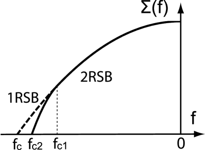
Figure 6: An example of complexity behavior (115) for $T_{2}<T_{1}$. The 1RSB solution is drawn by the dashed line. Both the 1RSB and the 2RSB solutions give the same result in the region $f>f_{c1}$. For the case $T_{1}\leq T_{2}$, $f_{c1}$ becomes smaller than $f_{c}$ and the 1RSB solution becomes exact in all the range of $f$.

4.4 Implications to Parisi’s breaking parameters

Before closing this section, we present some arguments about the breaking parameters in the Parisi solution. In the 1RSB formulation, for high temperature, substitution of $m=1$ in $f_{\rm 1RSB}(m)$ gives the correct equilibrium free energy. On the other hand, at low temperature, the breaking parameter $m$ is set as $m=m^{*}\leq 1$, which is determined by $\left.\partial f_{\rm 1RSB}(m)/\partial m\right|_{m=m^{*}}=0$. This condition corresponds to the vanishing point of complexity as written in [11].

In the 2RSB formulation the same situation occurs as well. For the first breaking parameter $m_{1}$, such a situation can be easily seen by using the parameterized form of $\Sigma_{1}$ (107), and the correspondence between $f_{\rm 2RSB}(m_{1},m_{2})$ and $g_{1}(x_{1},x_{2})$ (97). In contrast, with respect to $m_{2}$, some delicate points emerge. In terms of the generating function $g_{1}$, the extremization condition of $f_{\rm 2RSB}(m_{1},m_{2})$ with respect to $m_{2}$ gives the condition

$$\left.\left(\frac{\partial g_{1}}{\partial x_{1}}-\frac{x_{2}}{x_{1}}\frac{\partial g_{1}}{\partial x_{2}}\right)\right|_{x_{1}=m_{1}/m_{2},x_{2}=m_{2}}=0.$$ (117)

Using expression (96) of $g_{1}(x_{1},x_{2})$, we can find that the left-hand side of (117) can be written as

$$\frac{\partial g_{1}}{\partial x_{1}}-\frac{x_{2}}{x_{1}}\frac{\partial g_{1}}{\partial x_{2}}=\frac{\sum_{\gamma_{1}^{*}}\widehat{\Sigma}_{2}(f^{*}|\gamma_{1}^{*})}{\sum_{\gamma_{1}^{*}}1},$$ (118)

where $\gamma_{1}^{*}$ represents the valleys in hierarchy 1 contributing to the saddle point, which is uniquely determined for given $x_{1}$ and $x_{2}$. Also, $\widehat{\Sigma}_{2}(f^{*}|\gamma_{1}^{*})$ denotes complexity for the free energy value $f^{*}$, which is the saddle point in a valley $\gamma_{1}^{*}$. This equation indicates that the extremization condition with respect to $m_{2}$ corresponds to freeze of degrees of freedom in hierarchy 2.

These considerations give a natural interpretation to the phase transitions of the case $T_{2}<T_{1}$. At $T=T_{1}$, the degrees of freedom in hierarchy 1 freeze and the phase transition from RS1-RS1 to 1RSB-RS1 occurs, which is expressed by the 2RSB solution as $f_{\rm 2RSB}(m_{1}=m_{1}^{*},m_{2}=1)$ with $m_{1}^{*}$ being the extremizer of $f_{\rm 2RSB}$ with respect to $m_{1}$. After that, freeze of hierarchy 2 also occurs at $T=T_{2}$ and the system goes to the 2RSB phase described by $f_{\rm 2RSB}(m_{1}=m_{1}^{*},m_{2}=m_{2}^{*})$ with the extremizer $m_{2}^{*}$.

However, for the case $T_{1}\leq T_{2}$, the above interpretation seems to give an inconsistency that the quantity (118) becomes negative for temperature range $T_{c}<T<T_{2}$, where the equilibrium free energy is given by $f_{\rm 2RSB}(m_{1}=1,m_{2}=1)$. This contradiction can be understood in the 2RSB description as follows. The condition $m_{1}=m_{2}$ leads to $x_{1}=1$ in (96). For $x_{1}=1$, the discrimination between the hierarchies 1 and 2 vanishes. In that case, $\widehat{\Sigma}_{2}(f|\gamma_{1})$ loses its meaning of complexity and can be negative as long as the total complexity $\Sigma(f)$ is positive. Hence, in such a case, we should return to the 1RSB solution by putting $m_{1}=m_{2}=m$ in the 2RSB solution and again take the extremization with respect to $m$. This consideration enables us to derive the correct equilibrium free energy in this case as well. The irrelevance of the negative second hierarchy entropy $s_{2}(T)$, mentioned in section 2.3, can be understood in the same manner.

Besides, the above discussions give an additional restriction about the relation among breaking parameters $\{m_{i}\}$. Let us suppose that we treat a $k$-step RSB system and have two neighboring extremizers of breaking parameters $m_{i}^{*}$ and $m_{i+1}^{*}$ holding $m_{i}^{*}>m_{i+1}^{*}$. The conventional Parisi solution has no constructive criterion for treating such a situation, though it requires the condition $m_{i}^{*}\leq m_{i+1}^{*}$. Our current consideration implies that, in such a case, we should forget the extremization conditions with respect to $m_{i}$ and $m_{i+1}$, and return to the $(k-1)$-step RSB by putting $m_{i}=m_{i+1}$. This is a supplemental but a new criterion in the Parisi solution.

5 Application of the spin representation – generalization of the GREM

The hierarchical structure introduced in section 3 is not specific to the REM, and we can implement such hierarchy to various spin models. In this section, we introduce several solvable mean-field models by referring to the spin representation of the GREM. We discuss that such models may have various hierarchical structure in phase diagram and clarify what are common properties of such hierarchical models.

5.1 Pure-ferromagnetic hierarchical Ising model

First we implement the hierarchical structure to the simplest Ising model with pure-ferromagnetic $p$-body interaction. We study the Hamiltonian

$$H=-\frac{NJ}{2}\sum_{\nu=1}^{K}a_{\nu}\left(\frac{1}{N_{\nu}}\sum_{i=1}^{N_{\nu}}\sigma_{i}^{z}\right)^{p}-\Gamma\sum_{i=1}^{N}\sigma_{i}^{x}.$$ (119)

The hierarchical structure is the same as that of (71). Here we add the term of transverse field $\Gamma$ to study the quantum effect. We introduce the magnetizations $m_{\nu}\sim\sum_{i=1}^{N_{\nu}}\sigma_{i}^{z}/N_{\nu}$ as order parameters and write the free energy per $N$:

$$f = \frac{J}{2}\sum_{\nu=1}^{K}(p-1)a_{\nu}m_{\nu}^{p}$$ (120)

$$-\frac{1}{N\beta}\ln\Tr\exp\left(N\beta J\sum_{\nu=1}^{K}\frac{a_{\nu}}{N_{\nu}}\tilde{m}_{\nu}\sum_{i=1}^{N_{\nu}}\sigma_{i}^{z}+\beta\Gamma\sum_{i=1}^{N}\sigma_{i}^{x}\right),$$

where $\tilde{m}_{\nu}=(p/2)(m_{\nu})^{p-1}$. The saddle-point equations at $K=2$ read

$$m_{1}=\frac{h_{1}+h_{2}}{\sqrt{(h_{1}+h_{2})^{2}+\Gamma^{2}}}\tanh\left(\beta\sqrt{(h_{1}+h_{2})^{2}+\Gamma^{2}}\right),$$ (121)

$$m_{2}=\frac{N_{1}}{N}m_{1}+\frac{N-N_{1}}{N}\frac{h_{2}}{\sqrt{h_{2}^{2}+\Gamma^{2}}}\tanh\left(\beta\sqrt{h_{2}^{2}+\Gamma^{2}}\right),$$ (122)

where $h_{\nu}=NJa_{\nu}\tilde{m}_{\nu}/N_{\nu}$.

We consider the limit $p\to\infty$. From the solution of the saddle-point equations, possible expressions of the free energy can be summarized as follows.

1. Paramagnetic (P) phase: $m_{1}=0$, $m_{2}=0$

   $$f=-\frac{1}{\beta}\ln(e^{\beta\Gamma}+e^{-\beta\Gamma}).$$ (123)

2. Ferromagnetic-paramagnetic (F-P) phase: $m_{1}=1$, $m_{2}=N_{1}/N$ ($\tilde{m}_{2}=0$)

   $$f=-\frac{J}{2}a_{1}-\frac{N-N_{1}}{N}\frac{1}{\beta}\ln(e^{\beta\Gamma}+e^{-\beta\Gamma}).$$ (124)

3. Ferromagnetic (F) phase: $m_{1}=1$, $m_{2}=1$

   $$f=-\frac{J}{2}.$$ (125)

For $T_{2}<T_{1}$ with

$$T_{\nu}=\frac{J}{2}\frac{a_{\nu}}{\ln\alpha_{\nu}},$$ (126)

the system enters the P, F-P and F phases as decreasing the temperature and/or the magnitude of the transverse field. We depict the behavior of the free energy at $\Gamma=0$ in figure 8 and the phase diagram in figure 8. For $T_{1}\leq T_{2}$ the F-P solution is irrelevant and we have a single transition between P and F phases.

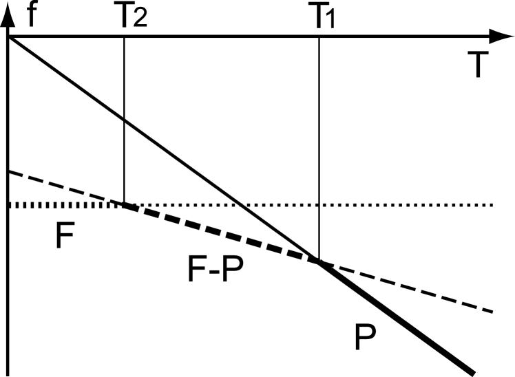
Figure 7: The free energy of the $K=2$ hierarchical pure ferromagnetic Ising model at $p=\infty$ and $\Gamma=0$ ($T_{2}<T_{1}$). The bold lines represent the free energy chosen as appropriate solution.

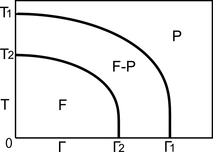
Figure 8: Phase diagram of the $K=2$ hierarchical pure ferromagnetic Ising model at $p=\infty$ ($T_{2}<T_{1}$). The critical fields at $T=0$ are given by $\Gamma_{\nu}=T_{\nu}\ln 2$.

Hence a partially ordered state at intermediate temperature region (F-P phase) is allowed in hierarchical models, which is significant because we have a hierarchical phase diagram even without randomness. We can also study the finite-$p$ case by solving (121) and (122) numerically. Typical behavior of magnetization in each hierarchy is shown in figure 9. In the case of $p=2$, we see that there is no sharp boundary between F and F-P phases, and at the paramagnetic phase transition point both the magnetizations go to zero at the same time. This behavior can generally be observed in the saddle-point equations: if we set $m_{2}=0$ in (121) and (122) we obtain $m_{1}=0$. When $p\geq 3$, we have a discontinuous behavior of magnetization in each hierarchy at phase transition points. For instance, $m_{2}$ jumps from a finite value to a different finite one at the transition point between F and F-P phases.

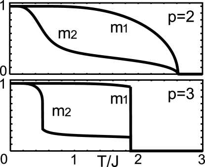
Figure 9: The magnetizations $m_{\nu}$ for the $K=2$ hierarchical Ising spin model at $p=2$ and 3. We set parameters as $\Gamma=0$, $a_{1}=0.5$ and $N_{1}/N=0.2$.

5.2 GREM with ferromagnetic interaction and transverse field

Next we go back to the spin representation of the GREM. We here study the effects of the ferromagnetic interactions and the transverse field on the model in section 3. The Hamiltonian is given by

$$H=-\sum_{\nu=1}^{K}\sum_{(i_{1}\cdots i_{p})}^{N_{\nu}}J_{i_{1}\cdots i_{p}}^{(\nu)}\sigma_{i_{1}}^{z}\cdots\sigma_{i_{p}}^{z}-\frac{N}{2}\sum_{\nu=1}^{K}J_{0}^{(\nu)}\left(\frac{1}{N_{\nu}}\sum_{i=1}^{N_{\nu}}\sigma_{i}^{z}\right)^{p}-\Gamma\sum_{i=1}^{N}\sigma_{i}^{x}.$$

(127)

We consider the case where the ferromagnetic interaction of each hierarchy is controlled by a single parameter $J_{0}$ as

$$J_{0}^{(\nu)}=J_{0}a_{\nu}.$$ (128)

One of the aims to study this hierarchical ferromagnetic interaction is to see the relation between the multi-critical points and the Nishimori line given for the standard REM by $J_{0}=\beta J^{2}$ [2, 34]. We are interested in how the multi-critical points on the Nishimori line are located in the present hierarchical model.

The models without the hierarchical structure were solved exactly [35, 36] and it is a straightforward task to generalize the method of calculation to the present case. The detail of the calculation is given in B, and the resultant phase diagrams for $K=2$ and $T_{2}<T_{1}$ are shown in figures 11 (at $\Gamma=0$) and 11 (at $J_{0}=0$). Two hierarchical structures are observed in each diagram: in figure 11 multiple-step RSB and partial ferromagnetic order, and in figure 11 multiple-step RSB and partial quantum effect. The fact that two multi-critical points are on the Nishimori line, as seen in figure 11, is one of the interesting results. In figure 11, we observe a new hierarchy in two paramagnetic phases. In the spin-glass model with transverse field, it is known that there exist two paramagnetic phases, called classical paramagnetic phase (denoted by CP in the figure) and quantum paramagnetic phase (by QP) caused by the quantum effect of the transverse field. By incorporating the hierarchical structure in interactions, we find these two paramagnetic phases form hierarchy (CP-CP, CP-QP, and QP-QP phases), or there appears a partially classical and partially quantum paramagnetic phase (CP-QP phase), as shown in the phase diagram.

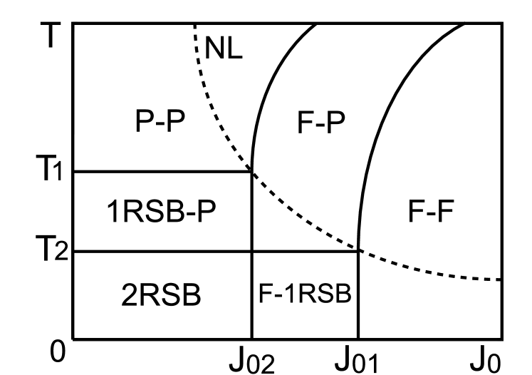
Figure 10: Phase diagram of the $K=2$ GREM with ferromagnetic interaction ($T_{2}<T_{1}$). The dashed line represents the Nishimori line $\beta J^{2}=J_{0}$. The critical ferromagnetic interactions at $T=0$ are given by $J_{0\nu}=J^{2}/T_{\nu}$.

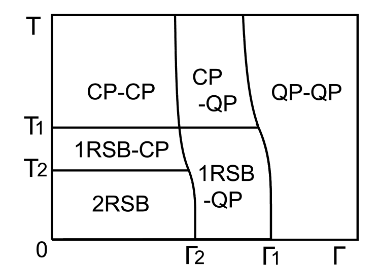
Figure 11: Phase diagram of the $K=2$ GREM with transverse field ($T_{2}<T_{1}$). The critical fields at $T=0$ are given by $\Gamma_{\nu}=JT_{\nu}/T_{\rm c}$.

6 Conclusions

In this paper we studied the GREM by the canonical ensemble formalism in conjunction with the replica method. To investigate hierarchical valley structure of free energy quantitatively, we generalized the notion of complexity and applied it to the GREM. The result not only reproduced the exact solution derived by the microcanonical ensemble formalism but also revealed how the higher step RSB is realized in this model, which is the main result of this work.

We expect applications of the analysis of generalized complexity to various problems. For example, the replica method still has some mysteries in the theory itself. In the standard description, the full-step RSB phase, which corresponds to the infinite-step RSB phase, is detected by a local instability of the saddle point, i.e. the so-called de Almeida-Thouless condition [37]. On the other hand, according to our current scheme, equilibrium transitions to spin-glass phases in a general $k$-step RSB system can be understood as entropy crises occurring in different hierarchies. The relation between these two descriptions is quite unclear. We hope that the generalized complexity developed in this paper will be useful to clarify this point and consequently become a convenient tool in the spin-glass theory. In addition, regarding multi-valley landscape of free energy, the method to extract information of a respective pure state on adiabatic evolution was proposed in a recent work [38]. In combination with their method, the application of our method to general spin-glass models with hierarchical valley structure may reveal complex equilibrium/dynamical properties of spin glasses.

We also proposed a $p$-body interacting spin-glass model having a hierarchical structure in the spin sites, which emulates the hierarchical structure of the GREM. By using the replica method, it was shown that this spin model has the same thermodynamic behavior as the GREM in a particular limit $p\to\infty$. This fact suggests that the proposed spin model exhibits the higher step RSB behavior controlled by hierarchy parameters, though it is still analytically tractable. For example, it would be interesting in the present model to examine the proof on the Guerra’s bound of the free energy [8] and to compare our analysis with mathematical studies [39]. Besides, the spin representation allows us to employ various methods developed for mean-field spin systems. One of possible applications is to incorporate the hierarchical structure to the TAP formulation. Such studies will be of great help to understand the higher step RSB systems.

Another benefit of the spin representation is that we can examine various physical effects on the hierarchical models. As examples, we introduced ferromagnetic bias and quantum effect by the transverse field to the models, and analyzed both in the pure and random cases. The resultant phase diagrams have very rich structures, and we found that partial order occurring in a part of hierarchies is not specific to spin-glass phases. Even in ferromagnetic phases, thermal and quantum fluctuations destroy the order and lead to multiple-step phase transitions in different hierarchies, which yields a number of multi-critical points in the random systems. All the multi-critical points are located on the Nishimori line, which implies a universal aspect of the Nishimori line.

As an additional application of the current work, the phase diagram obtained here is also useful for discussion of signal processing in information theory. In [40] the relation between the GREM and the hierarchical random code ensemble was pointed out. We have applied our result to the problem of the hierarchical random code ensemble and shown that transitions of distortion in lossy data compression and that of error probability in channel coding discussed there can be reinterpreted by the higher step RSB. The details will be reported soon.

Appendix A RSB phases in the spin representation of the GREM

We study the hierarchical spin model (71) at $K=2$ and $p\to\infty$. We substitute possible saddle-point solutions to (81) and show that the present model is equivalent to the GREM. The equivalence of the simplest RS1-RS1 solution has been discussed in the main body of the present paper. Here we study the 1RSB-RS1 and the 2RSB solutions as nontrivial cases. We assume $T_{2}<T_{1}$ where the critical temperatures are defined in (8), which is the situation where the phase transitions occur at $T_{1}$ and $T_{2}$.

A.1 1RSB-RS1

From 1RSB-RS1 solution $q_{1}^{ab}=\delta_{m}(a,b)$ and $q_{2}^{ab}=(N_{1}/N)q_{1}^{ab}$, following the standard Parisi algebra, we have $\sum_{a>b}^{n}(q_{1}^{ab})^{p}=n(m-1)/2$ and the second line of (81) as

$$N_{1}\ln\Tr\exp\left(N\beta^{2}J^{2}\sum_{\nu=1}^{2}\frac{a_{\nu}}{N_{\nu}}\sum_{a>b}^{n}\tilde{q}_{\nu}^{ab}\sigma^{a}\sigma^{b}\right)$$ (129)

$$= N_{1}\ln\Tr\exp\left\{\frac{\beta^{2}J^{2}}{4}\frac{N}{N_{1}}pa_{1}\sum_{{\rm B}}^{n/m}\left(\sum_{a\in{\rm B}}^{m}\sigma^{a}\right)^{2}-\frac{\beta^{2}J^{2}}{4}\frac{N}{N_{1}}pa_{1}n\right\}$$

$$= -Nn\frac{\beta^{2}J^{2}}{4}pa_{1}+N_{1}\ln\left\{2\exp\left(\frac{\beta^{2}J^{2}}{4}\frac{N}{N_{1}}pa_{1}m^{2}\right)\right\}^{n/m}.$$

In the last equation we take the limit $p\to\infty$ where all spins in block ${\rm B}$ take same values $1$ or $-1$. Then, we obtain the result of the GREM (36).

A.2 2RSB

Now we consider the 2RSB solution $q_{1}^{ab}=\delta_{m_{1}}(a,b)$ and $q_{2}^{ab}=\delta_{m_{2}}(a,b)$. The 1RSB-1RSB solution can be obtained by setting $m_{1}=m_{2}$. The first and the third lines of (81) are calculated in the same way as the previous case as

$$-\frac{N\beta^{2}J^{2}}{2}(p-1)\sum_{\nu=1}^{2}a_{\nu}\sum_{a>b}(q_{\nu}^{ab})^{p}+\frac{Nn\beta^{2}J^{2}}{4}$$

$$= \frac{Nn\beta^{2}J^{2}}{4}\left\{(m_{1}-p(m_{1}-1))a_{1}+(m_{2}-p(m_{2}-1))a_{2}\right\},$$

$$(N-N_{1})\ln\left\{\Tr\exp\left(N\beta^{2}J^{2}\frac{a_{2}}{N}\sum_{a>b}\tilde{q}^{ab}_{2}\sigma^{a}\sigma^{b}\right)\right\}$$

$$= (N-N_{1})n\frac{\beta^{2}J^{2}}{4}p(m_{2}-1)a_{2}+Nn\frac{\ln\alpha_{2}}{m_{2}},$$ (131)

where we use the relation $(N-N_{1})\ln 2=N\ln\alpha_{2}$ in the second equation. The second line in (81) is written as

$$N_{1}\ln\left\{\Tr\exp\left(N\beta^{2}J^{2}\sum_{\nu=1}^{2}\frac{a_{\nu}}{N_{\nu}}\sum_{a>b}^{n}\tilde{q}_{\nu}^{ab}\sigma^{a}\sigma^{b}\right)\right\}$$ (132)

$$= -Nn\frac{\beta^{2}J^{2}}{4}pa_{1}-N_{1}n\frac{\beta^{2}J^{2}}{4}pa_{2}$$

$$+N_{1}\ln\Tr\exp\left\{N\frac{\beta^{2}J^{2}}{4}p\sum_{\nu=1}^{2}\frac{a_{\nu}}{N_{\nu}}\sum_{{\rm B}_{\nu}}^{n/m_{\nu}}\left(\sum_{a\in{\rm B}_{\nu}}^{m_{\nu}}\sigma_{a}\right)^{2}\right\}.$$

The trace over spin variables in the last term is turned out to be a formidable task for arbitrary $m_{1}$ and $m_{2}$. Here we impose the Parisi ansatz $m_{1}\geq m_{2}$ and the condition of integer $m_{1}/m_{2}$. Then, we can perform the trace at $p\to\infty$ as

$$N_{1}\ln\Tr\exp\left\{N\frac{\beta^{2}J^{2}}{4}p\sum_{\nu=1}^{2}\frac{a_{\nu}}{N_{\nu}}\sum_{{\rm B}_{\nu}}^{n/m_{\nu}}\left(\sum_{a\in{\rm B}_{\nu}}^{m_{\nu}}\sigma_{a}\right)^{2}\right\}$$ (133)

$$= N_{1}\ln\left\{2^{n/m_{1}}\exp\left(N\frac{\beta^{2}J^{2}}{4}p\frac{a_{1}}{N_{1}}m_{1}n+N\frac{\beta^{2}J^{2}}{4}p\frac{a_{2}}{N}m_{2}n\right)\right\}.$$

Combining everything, we finally obtain the same result (52) as the GREM.

Appendix B GREM with ferromagnetic interaction and transverse field

We study (127). Under the saddle point evaluation, the average of the replicated partition function is written as

$$[Z^{n}] = \exp\left\{-\frac{N\beta J_{0}}{2}(p-1)\sum_{\nu=1}^{K}a_{\nu}\sum_{a=1}^{n}(m_{\nu}^{a})^{p}\right.$$ (134)

$$-\frac{N\beta^{2}J^{2}}{4}(p-1)\sum_{\nu=1}^{K}a_{\nu}\left(\sum_{a=1}^{n}(\chi_{\nu}^{a})^{p}+\sum_{a\neq b}^{n}(q_{\nu}^{ab})^{p}\right)$$

$$+\ln\Tr\exp\left(N\beta J_{0}\sum_{\nu=1}^{K}\frac{a_{\nu}}{N_{\nu}}\sum_{a=1}^{n}\tilde{m}_{\nu}^{a}\sum_{i=1}^{N_{\nu}}S_{zi}^{a}\right.$$

$$+\frac{N\beta^{2}J^{2}}{2}\sum_{\nu=1}^{K}\frac{a_{\nu}}{N_{\nu}}\sum_{a=1}^{n}\tilde{\chi}_{\nu}^{a}\sum_{i=1}^{N_{\nu}}S_{zi}^{a}S_{zi}^{a}$$

$$\left.\left.+N\beta^{2}J^{2}\sum_{\nu=1}^{K}\frac{a_{\nu}}{N_{\nu}}\sum_{a>b}^{n}\tilde{q}_{\nu}^{ab}\sum_{i=1}^{N_{\nu}}S_{zi}^{a}S_{zi}^{b}+\sum_{a=1}^{n}\Gamma\sum_{i=1}^{N}S_{xi}^{a}\right)\right\}.$$

We use the imaginary time formalism, where the classical spin variables $\mbox{\boldmath$S$}_{i}(\tau)$ are defined for each imaginary time $\tau$ between 0 and $\beta$. $S_{zi}=(1/\beta)\int_{0}^{\beta}d\tau S_{zi}(\tau)$ and the trace represents multiple integrals over spin variables with a proper measure [41]. The order parameters are introduced as $m_{\nu}^{a}\sim\sum_{i=1}^{N_{\nu}}S_{zi}^{a}(\tau)/N_{\nu}$, $\chi_{\nu}^{a}\sim\sum_{i=1}^{N_{\nu}}S_{zi}^{a}(\tau)S_{zi}^{a}(\tau^{\prime})/N_{\nu}$, and $q_{\nu}^{ab}\sim\sum_{i=1}^{N_{\nu}}S_{zi}^{a}(\tau)S_{zi}^{b}(\tau^{\prime})/N_{\nu}$. We also use $\tilde{m}_{\nu}^{a}=(p/2)(m_{\nu}^{a})^{p-1}$ and so on. The deviation of the parameter $\chi$ from unity represents the magnitude of the quantum effect. At the limit of $p\to\infty$, the RS ansatz for $m_{\nu}^{a}$ and $\chi_{\nu}^{a}$ and the static approximation for all parameters are justified [36]. By taking possible solutions into account, we can classify the phases at $K=2$ as summarized below. We consider two cases $\Gamma=0$ and $J_{0}=0$ for simplicity.

B.1 Ferromagnetic interaction

In the case of the classical limit $\Gamma=0$, we have six phases. The RS1-RS1 (paramagnetic), 1RSB-RS1 and 2RSB phases are the same as the previous calculation with $J_{0}=0$. In addition, we have three new phases including $J_{0}$ in their free energies:

• F-P: $(m_{1},m_{2})=(1,N_{1}/N)$, $(q_{1}^{ab},q_{2}^{ab})=(1,\delta_{ab})$

  $$f=-\frac{J_{0}}{2}a_{1}-\frac{1}{\beta}\ln\alpha_{2}-\frac{\beta^{2}J^{2}}{4}a_{2}.$$ (135)

• F-F: $(m_{1},m_{2})=(1,1)$, $(q_{1}^{ab},q_{2}^{ab})=(1,1)$

  $$f=-\frac{J_{0}}{2}.$$ (136)

• F-1RSB: $(m_{1},m_{2})=(1,N_{1}/N)$, $(q_{1}^{ab},q_{2}^{ab})=(1,\delta_{m}(a,b))$

  $$f=-\frac{J_{0}}{2}a_{1}-J\sqrt{a_{2}\ln\alpha_{2}}.$$ (137)

Comparing these free energies, we obtain the phase diagram in figure 11.

B.2 Transverse field

When $J_{0}=0$, we have phase transitions to the quantum paramagnetic phase with $\chi\neq 1$. We obtain the following three new quantum phases and the phase diagram in figure 11.

• Classical P- Quantum P (CP-QP): $(\chi_{1},\chi_{2})=(1,N_{1}/N)$, $(q_{1}^{ab},q_{2}^{ab})=(\delta_{ab},\delta_{ab})$

  $$f=-\frac{J_{0}}{2}a_{1}-\frac{1}{\beta}\ln\alpha_{2}-\frac{\beta^{2}J^{2}}{4}a_{2}.$$ (138)

• QP-QP: $(\chi_{1},\chi_{2})=(\tanh\beta\Gamma/\beta\Gamma,\tanh\beta\Gamma/\beta\Gamma)$, $(q_{1}^{ab},q_{2}^{ab})=(\delta_{ab},\delta_{ab})$

  $$f=-\frac{1}{\beta}\ln\left(e^{\beta\Gamma}+e^{-\beta\Gamma}\right).$$ (139)

• 1RSB-QP: $(\chi_{1},\chi_{2})=(1,N_{1}/N)$, $(q_{1}^{ab},q_{2}^{ab})=(\delta_{m}(a,b),\delta_{ab})$

  $$f=-J\sqrt{a_{1}\ln\alpha_{1}}-\frac{N-N_{1}}{N}\frac{1}{\beta}\ln\left(e^{\beta\Gamma}+e^{-\beta\Gamma}\right).$$ (140)

References

References

• [1] Mézard M, Parisi G and Virasoro M A 1987 Spin Glass Theory and Beyond (Singapore: World Scientific)
• [2] Nishimori H 2001 Statistical Physics of Spin Glasses and Information Processing: An Introduction (Oxford: Oxford University Press)
• [3] Mézard M and Montanari A 2009 Information, Physics, and Computation (Oxford: Oxford University Press)
• [4] Sherrington D and Kirkpatrick S 1975 Phys. Rev. Lett.35 1792
• [5] Parisi G 1980 J. Phys. A: Math. Gen.13 L115
• [6] Parisi G 1980 J. Phys. A: Math. Gen.13 1101
• [7] Parisi G 1980 J. Phys. A: Math. Gen.13 1887
• [8] Guerra F 2003 Commun. Math. Phys. 233 1
• [9] Talagrand M 2006 Ann. Math. 163 221
• [10] Bray A J and Moore M A 1980 J. Phys. C: Solid State Phys.13 L469
• [11] Monasson R 1995 Phys. Rev. Lett.75 2847
• [12] Thouless D J, Anderson P W and Palmer R G 1977 Phil. Mag. 35 3271
• [13] Cavagna A, Garrahan J P and Giardina I 1999 J. Phys. A: Math. Gen.32 711
• [14] Cavagna A, Giardina I, Parisi G and Mézard M 2003 J. Phys. A: Math. Gen.36 1175
• [15] Annibale A, Cavagna A, Giardina I, Parisi G and Trevigne E 2003 J. Phys. A: Math. Gen.36 10937
• [16] Crisanti A, Leuzzi L, Parisi G and Rizzo T 2003 Phys. Rev.B 68 174401
• [17] Crisanti A, Leuzzi L, Parisi G and Rizzo T 2004 Phys. Rev. Lett.92 127203
• [18] Crisanti A, Leuzzi L, Parisi G and Rizzo T 2004 Phys. Rev.B 70 064423
• [19] Tonosaki Y, Takeda K and Kabashima Y 2007 Phys. Rev.B 75 094405
• [20] Derrida B 1980 Phys. Rev. Lett.45 79
• [21] Derrida B 1981 Phys. Rev.B 24 2613
• [22] Gross D J and Mézard M 1984 Nucl. Phys.B 240 431
• [23] Derrida B 1985 J. PhysiqueLett. 46 L401
• [24] Derrida B and Gardner E 1986 J. Phys. C: Solid State Phys.19 2253
• [25] Saakian D B 1998 JETP Lett. 67 440
• [26] Gardner E and Derrida B 1989 J. Phys. A: Math. Gen.22 1975
• [27] Ogure K and Kabashima Y 2004 Prog. Theor. Phys. 111 661
• [28] Ogure K and Kabashima Y 2009 J. Stat. Mech. P03010
• [29] Ogure K and Kabashima Y 2009 J. Stat. Mech. P05011
• [30] Franz S, Jörg T and Parisi G 2009 J. Stat. Mech. P02002
• [31] Castellana M, Decelle A, Franz S, Mézard M and Parisi G 2010 Phys. Rev. Lett.104 127206
• [32] Montanari A, Ricci-Tersenghi F and Semerjian G 2008 J. Stat. Mech. P04004
• [33] Obuchi T and Kabashima Y 2009 J. Stat. Mech. P12014
• [34] Nishimori H 1981 Prog. Theor. Phys. 66 1169
• [35] Goldschmidt Y Y 1990 Phys. Rev.B 41 4858
• [36] Obuchi T, Nishimori H and Sherrington D 2007 J. Phys. Soc. Japan76 054002
• [37] de Almeida J R L and Thouless D J 1978 J. Phys. A: Math. Gen.11 983
• [38] Zdeborová L and Krzakala F 2010 Phys. Rev.B 81 224205
• [39] Bolthausen E and Bovier A (eds) 2007 Spin Glasses (Lecture Notes in Mathematics vol 1900, Berlin: Springer)
• [40] Merhav N 2009 IEEE Trans. Inf. Theory 55 1250
• [41] Takahashi K 2007 Phys. Rev.B 76 184422