The minimal time of dynamic evolution to an arbitrary state

Abstract

Two bounds on the minimal time of dynamic rotating an initial state by arbitrary angles have been obtained. These bounds have been applied to study the evolutions in the Hadamard-Walsch gate, the Control-NOT quantum gate, and the Grover algorithm.

Introduction. In the realm of quantum evolution, an important question is to know the time that an operation needs, i.e., how fast is the operation. The similar question in classical physics has been almost solved, but in quantum physics it remains a puzzling problem. In 1998, Margolus and Levitin Margolus have proved that the shortest time $\tau$ a quantum state takes to its orthogonal state is bounded by the inequality (the MV bound hereafter)

$$\tau\bar{E}\geq\frac{h}{4},$$ (1)

where $\bar{E}$ denotes the arithmetic average energy $\bar{E}=\langle\psi|H|\psi\rangle$ of an arbitrary quantum state $|\psi\rangle$ in a given system with Hamiltonian $H$. It should be noticed that the minimal energy of this quantum system is set to 0. On the other hand, Fleming Fleming , Anandan and Aharanov Anandan and Vaidman Vaidman have shown separately that the shortest time needed to orthogonalize a quantum state is bounded by another inequality (referred to as FAAV bound hereafter),

$$\tau\Delta E\geq\frac{h}{4},$$ (2)

where $\Delta E$ denotes the standard error of energy $\Delta E=\sqrt{\langle\psi|(H^{2}-{\bar{E}}^{2})|\psi\rangle}$.

Meanwhile, the shortest time of applying an outer operation on a system has been discussed in bi11 ; bi12 . The MV bound and FAAV bound have been derived in some entangled and non-entangled systems bi8 ; bi9 ; bi10 . In addition, a kind of equations that is equivalent to the MV bound in Eq. (2) and the FAAV bound in Eq. (1) have been established bi13 ; bi14 ; bi15 . Zielinski and Zych have made a generalization from which one could derive more details about $\tau$, using energy moments bi16 . The problem has attracted much attention recently and many related problems have been studied bi17 ; bi18 ; bi19 ; bi20 ; bi21 ; bi22 ; bi23 ; bi24 ; bi25 ; bi26 ; bi27 . Levitin and Toffoli Levitin recently found that the MV bound and FAAV bound are tight, and both are satisfied by a quantum state that has the property $\bar{E}=\Delta E$. They also discussed what would happen when $\bar{E}\neq\Delta E$.

However, the shortest time that a state takes to evolve to an arbitrary state is more general and frequently met in practice. Many questions remain to be answered. For example, does it satisfy the same inequality? If not, is there a new constraint? It is essential to answer these questions and to develop results for this more general case and still retaining the results in (1) and (2) when for evolution to an orthogonal state. Estimating the evolution time to an arbitrary state is important to study how fast a quantum computer can run, because a quantum computer has a great deal of operations that changes a state to various states. Giovannetti, Lloyd, and Maccone studied this problem and gave the following bound (the GLM-$\alpha$ and GLM-$\beta$ bounds hereafter) bi8 ,

$${\rm max}\left(\alpha(\epsilon){\pi\hbar\over 2E},\beta(\epsilon){\pi\hbar\over 2\Delta E}\right),$$ (3)

where $\epsilon=F(\rho,\rho(t))$ is the fidelity between the initial and final state and

$$\beta(\epsilon)={2\over\pi}\arccos(\sqrt{\epsilon}),$$ (4)

and $\alpha(\epsilon)$ is determined by a sets of equations.

In this paper, we derive three bounds for the problem with a different approach. The results are simple and intuitive. Then we apply the bounds to study the evolutions of two quantum gates and the Grover’s quantum searching algorithm Grover .

The GLM-$\beta$ bound. We assume that a given quantum system evolves from an initial state $|\psi(0)\rangle$ into $|\psi(\tau)\rangle$ after time $\tau$ governed by the Schrödinger equation

$$i\hbar\frac{\partial}{\partial t}|\psi(t)\rangle=H|\psi(t)\rangle,$$ (5)

where $H$ is the Hamiltonian of the system. Denote $\theta=\theta(0\to\tau)\in[0,\;\pi/2]$, which satisfies

$$\cos\theta(0\to\tau)=|\langle\psi(0)|\psi(\tau)\rangle|,$$ (6)

then we have the first bound

$$\Delta E\cdot\tau\geq\theta\hbar.$$ (7)

The mean-energy bounds. Denoting $\bar{E}$ the average energy of the system having a time-independent Hamiltonian $H$ and a minimal energy 0, then one has the mean-energy bound (Mean-E bound) as follows

$$\bar{E}\cdot\tau\geq\frac{h}{4}\left[1-\sqrt{1+\dfrac{4}{\pi^{2}}}\cos\theta\right].$$ (8)

Now we derive the Mean-E bound. The proof is similar to the one by Margolus and Levitin Margolus . Expanding the state $|\psi(t)\rangle$ in terms of the energy eigenstates $|\psi_{n}\rangle$ with nonnegative eigenvalues $E_{n}$, we obtain

$$|\psi(t)\rangle=\sum_{n=1}^{\infty}c_{n}\exp\left(-i\frac{E_{n}}{\hbar}t\right)|\psi_{n}\rangle,$$ (9)

where the coefficients $\{c_{n}\}$ are complex constants satisfying $\sum\limits_{n=1}^{\infty}|c_{n}|^{2}=1$. Let

$$S(\tau)=\langle\psi(0)|\psi(\tau)\rangle=\sum_{n=1}^{\infty}|c_{n}|^{2}\exp\left(-i\frac{E_{n}}{\hbar}\tau\right),$$ (10)

and use the inequality

$$\cos x\geq 1-\dfrac{2}{\pi}(x+\sin x),$$

one can derive

$$\mathrm{Re}S(\tau) \geq \sum_{n=1}^{\infty}\left(1-\frac{2E_{n}\tau}{\pi\hbar}-\frac{2}{\pi}\sin\frac{E_{n}\tau}{\hbar}\right)|c_{n}|^{2}$$ (11)

$$= 1-\frac{4\bar{E}\tau}{h}+\frac{2}{\pi}\mathrm{Im}S(\tau),$$

i.e.

$$\bar{E}\cdot\tau\geq\frac{h}{4}\left[1-\left(\mathrm{Re}S(\tau)-\frac{2}{\pi}\mathrm{Im}S(\tau)\right)\right].$$ (12)

In general, $S(\tau)$ has the form $S(\tau)=\cos\theta\exp(i\varphi)$ and $\varphi$ is a complex phase depending on the evolution time $\tau$. Thus,

$$\mathrm{Re}S(\tau)-\frac{2}{\pi}\mathrm{Im}S(\tau) = \cos\theta\left(\cos\varphi-\frac{2}{\pi}\sin\varphi\right)$$ (13)

$$\leq \sqrt{1+\frac{4}{\pi^{2}}}\cos\theta,$$

from which and inequality (12) one can obtain bound (8).

If the system has a minimal energy $E_{\rm min}\neq 0$, the bound will be replaced with the Mean-Min-E bound

$$(\bar{E}-E_{\rm min})\cdot\tau\geq\frac{h}{4}\left[1-\sqrt{1+\dfrac{4}{\pi^{2}}}\cos\theta\right].$$ (14)

If the system has a maximum energy $E_{\rm max}$, it is easy to prove a similar bound, the Max-Mean-E bound,

$$(E_{\rm max}-\bar{E})\cdot\tau\geq\frac{h}{4}\left[1-\sqrt{1+\dfrac{4}{\pi^{2}}}\cos\theta\right].$$ (15)

Furthermore, if the system has both maximum and minimal energies, it is obvious

$$\min\{E_{\rm max}-\bar{E},\bar{E}-E_{\rm min}\}\leq\delta E\equiv\frac{E_{\rm max}-E_{\rm min}}{2},$$ (16)

where $\delta E$ is the half-width of energy. One obtain a new bound, the Max-Min bound

$$\delta E\cdot\tau\geq\frac{h}{4}\left[1-\sqrt{1+\dfrac{4}{\pi^{2}}}\cos\theta\right].$$ (17)

A tighter bound. If we use another inequality

$$\cos x\geq c-bx+a\sin x$$ (18)

it can be derived that

$$\mathrm{Re}S(\tau) \geq \sum_{n=1}^{\infty}\left(c-\frac{bE_{n}\tau}{\hbar}-a\sin\frac{E_{n}\tau}{\hbar}\right)|c_{n}|^{2}$$ (19)

$$= c-\frac{b\bar{E}\tau}{\hbar}+a\mathrm{Im}S(\tau),$$

If we choose $a$, $b$, and $c$ properly, when $x>0$, there would be only one $x$ satisfies the “=” in (18) and others satisfy “$>$”, and this process will make the bound tight. Now assuming $a$, $b$ and $c$ are chosen as above, there should be a relation $a=a(b,c)$, so it can be derived

$$\bar{E}\tau\geq\frac{\hbar}{b}(c-\sqrt{1+a(b,c)^{2}}\cos{\theta}).$$ (20)

Thus we have a tighter bound by maximizing over two parameters, the BC bound,

$$\bar{E}\tau\geq\max_{b,c}{(\frac{\hbar}{b}(c-\sqrt{1+a(b,c)^{2}}\cos{\theta}))}.$$ (21)

Usually one has to compute the BC bound numerically. However, to a good extent, the above bound can be approximated as

$$\frac{\bar{E}\tau}{\hbar}\geq 1.57-1.847\cos{\theta}+0.372\cos^{2}{\theta}-0.0958\cos^{3}{\theta}.$$ (22)

It is a good estimation, and has only maximally $0.0005\frac{\bar{E}\tau}{\hbar}$ difference from the reality.

Compared to the GLM-$\beta$ bound in Ref.bi8 , when $\theta=\frac{\pi}{3}$, the BC bound is about $4.5\%$ tighter; and about $8\%$ tighter when $\theta=\frac{5\pi}{12}$. Fig. 1 shows the comparisons of the three bounds: the GLM-$\beta$ bound, the Mean-E bound and the BC bound. It is shown that the BC bound is always the tightest. When $\sin{\theta}$ is small ($\cos{\theta}<0.395$, approximately), the Mean-E bound is tighter than the GM-$\beta$ bound. However for small evolution, the Mean-E bound is no longer valid.

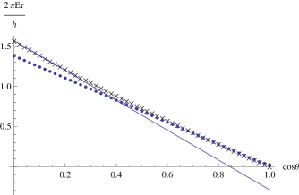
Figure 1: Comparisons among the various bounds: “$\times$” denotes the BC bound in Eq. (21), the line denotes the Mean-Min-E bound in (14) and the dots denote the GLM-$\alpha$ bound in Ref. bi8 . The BC bound in (21) is always better than the GLM-$\alpha$ bound. Meanwhile, the Mean-Min-E bound in (14) is a good estimation when $\theta$ is near $\frac{\pi}{2}$, but not good around 0. The Mean-Min-E bound in (14) is better than GLM-$\alpha$ bound when $\cos{\theta}$ is small ($\cos{\theta}<0.395$, approximately).

Discussions. One can find that bound (7) is similar to bound. When $\theta\to\pi/2$, the GLM-$\beta$ bound in (7) and the Mean-E bound in (8) approach to the MV bound in (2) and FAAV bound in (1) respectively. However the Mean-E bound(8) is not a good bound when $\theta$ is small, it even has a minus lower limit and the bound becomes trivial. However the BC bound is a tighter bound.

It is easy to show that bound (7) is the tightest when $\tau\to\mathrm{d}t$ and $\theta\to\theta(0\to\mathrm{d}t)$ for an infinitesimal evolution, because the bound inequality tends to equality (LABEL:eqader). So there exists no bound such as $\bar{E}\cdot\tau\geq\theta\hbar$ unless $\bar{E}\geq\Delta E$. In fact, because $1-\sqrt{1+\frac{4}{\pi^{2}}}\cos\theta\leq 1-\cos\theta\leq 2\theta/\pi$ for any $\theta\in[0,\pi/2]$, the Mean-E bound (8) is weaker than the GLM-$\beta$ bound in (7) when $\theta\neq\pi/2$ unless $\bar{E}<\Delta E$.

The Max-Min bound in (17) looks useful when one does not know details about a system except the width of energy spectrum. Indeed the GLM-$\beta$ bound (7) with $\Delta E$ substituted by $\delta E$, i.e.

$$\delta E\cdot\tau\geq\theta\hbar,$$ (23)

is the better choice, because one can simply prove $\delta E\geq\Delta E$.

The GLM-$\beta$ bound in (7) and the Mean-E bound in (8) work independently on the same quantum system, and each of them confines $\tau$ to some extent. But in general the lower limit can not be reached at the same time. An important question arises: Can these bounds be attained so that there are not any stronger inequalities? Levitin and Toffoli Levitin have proved that there exist states by which bound inequality (2) or (1) (the tighter one) can be asymptotically approached arbitrarily. It is obvious that the lower limit of (8) cannot be reached when $\theta$ is small. On the other hand, the two-level state $(|0\rangle+|E\rangle)/\sqrt{2}$ with the superposition of the ground state $|0\rangle$ and the eigenstate $|E\rangle$ of energy $E$ enables $\tau=\theta\hbar/\Delta E$ at any time, where $\Delta E=\delta E=\bar{E}=E/2$. In general, it cannot be ensured that an arbitrary state should reach the lower limit of bound (7) for all $\theta>0$. But it is sure for an infinitesimal evolution. So bound (7) is a good estimation about an evolution with very short $\tau$ and very small $\theta$.

If a state has the maximum $\Delta E$, the state should have the form $[|E_{\rm min}\rangle+\exp(i\phi)|E_{\rm max}\rangle]/\sqrt{2}$, where $E_{\rm min}$ and $E_{\rm max}$ are the minimal and maximum energies of the system, and $\phi$ is an arbitrary phase. The state reaches the lower limit of bound (7) for any $\theta$. But the maximum energy deviation is not necessary for reaching the lower limit. On the other hand, if a state reaches the lower limit of bound (7) for any $\theta$, one necessary condition is that the state can evolve to an orthogonal state.

Application. We apply the GLM-$\beta$ bound in (7) to estimate the evolution of quantum gates. The Walsh-Hadamard transformation is a well-known one-qubit gate, which transform qubit state $|0\rangle$ to $(|0\rangle+|1\rangle)/\sqrt{2}$ and $|1\rangle$ to $(|0\rangle-|1\rangle)/\sqrt{2}$. We consider the evolution from an initial state $|0\rangle$ to the final state $(|0\rangle+|1\rangle)/\sqrt{2}$ (It is obvious that $\theta=\pi/4$ ) in a one-qubit system having a general Hamiltonian

$$H=-\varepsilon\sigma_{3}+\delta_{1}\sigma_{1}+\delta_{2}\sigma_{2},$$

where $\sigma_{1},\;\sigma_{2},\;\sigma_{3}$ are the three Pauli matrices. Let $\delta_{1}=\delta\cos\phi$, $\delta_{2}=\delta\sin\phi$ and $\sin\beta=\delta/\sqrt{\varepsilon^{2}+\delta^{2}}$, it is easy to check that the system has $\Delta E=\delta$ and the state at an arbitrary time

$$|\psi(t)\rangle = (\cos\frac{\sqrt{\varepsilon^{2}+\delta^{2}}t}{\hbar}+i\cos\beta\sin\frac{\sqrt{\varepsilon^{2}+\delta^{2}}t}{\hbar})|0\rangle$$ (24)

$$+ i\mathrm{\exp}(i\phi)\sin\beta\sin\frac{\sqrt{\varepsilon^{2}+\delta^{2}}t}{\hbar}|1\rangle.$$

By selecting a suitable phase $\phi$ (suppose that $\delta_{1}$ and $\delta_{2}$ can be adjusted) and time $\tau$, one can carry out the Walsh-Hadamard transformation on the initial state $|0\rangle$, where the evolution time $\tau$ satisfies

$$\tan\left(\frac{\sqrt{\varepsilon^{2}+\delta^{2}}}{\hbar}\tau\right)=\sqrt{\frac{\delta^{2}+\varepsilon^{2}}{\delta^{2}-\varepsilon^{2}}}.$$

It is obvious that the transformation cannot be realized if $\delta<\varepsilon$. Hence one has the extent of time evolution

$$\Delta E\cdot\tau=\frac{\hbar\arcsin\sqrt{\frac{1+(\varepsilon/\delta)^{2}}{2}}}{\sqrt{1+(\varepsilon/\delta)^{2}}}\in\left[h/8,\;h/2\sqrt{2}\right].$$

If the system has a very large $\delta\gg\varepsilon$, the lower limit of bound (7) can be reached asymptotically while the lower limit of bound (14) can not be reached. Larger is $\delta$, faster is the evolution, irrespective of the detailed distribution of $\delta_{1}$ and $\delta_{2}$. It is interesting that bound (14) can be tighter when $\delta$ is small, because

$$\bar{E}-E_{\rm min}=\sqrt{\varepsilon^{2}+\delta^{2}}-\varepsilon\leq\Delta E.$$

Another example is the important two-qubit gate—CNOT gate, $|0\rangle\langle 0|\otimes I^{2}+|1\rangle\langle 1|\otimes\sigma^{2}_{1}$, where the superscripts denote the qubit numbering. The CNOT gate is important in quantum information. Assume that the two-qubit system has a simple intrinsic Hamiltonian

$$H=-\varepsilon\left(\sigma_{3}^{1}+\sigma_{3}^{2}-\sigma_{3}^{1}\sigma_{3}^{2}\right),$$

where the superscripts denote the qubit numbering. The CNOT gate can be realized in three steps: (i) apply a Walsh-Hadamard transformation to the second qubit through using an additional Hamiltonian $H_{\rm 2}=\delta\sigma_{2}^{2}$ (corresponding a radio frequency pulse along the $x$-axis), where $\delta$ is much larger so that the intrinsic evolution can be neglected. (ii) the state evolves with the intrinsic Hamiltonian for a period of $\tau_{2}=h/(8\varepsilon)$. (iii) apply an inverse Walsh-Hadamard transformation to the second qubit. It is obvious that steps (i), (iii) can reach the lower limit of bound (7) asymptotically, while the evolution of step (ii) almost does not. Here one has

$$\Delta E\cdot\tau=\frac{\sqrt{3}h}{8}>\hbar\theta=\frac{h}{6}.$$

Although the initial state and the final state spans an angle $\theta=\pi/3$, CNOT gate cannot be realized without additional operations, because the initial state is an eigenstate of the intrinsic Hamiltonian. If the system has the intrinsic Hamiltonian $H=\varepsilon(I^{1}-\sigma_{3}^{1})\sigma_{2}^{2}$, CNOT gate can be realized through a intrinsic evolution for a period of $\tau=h/(8\varepsilon)$, which does not reach the lower limit of bound (7), either. One has $\Delta E\cdot\tau=h/4>\hbar\theta=h/6$.

An interesting example is the well-known Grover’s quantum searching algorithm. It contains about $\frac{\pi}{4}\sqrt{N}$ Grover iterations, where $N$ is the dimension of the database and each iteration rotates a state by $2\arcsin\frac{1}{\sqrt{N}}$ Grover ; Grover2 . If $N$ is large enough, which is common for an actual database, one has $\theta\sim 2/\sqrt{N}$. Increasing $N\to\infty$, the Grover iteration can possibly be replaced by an infinitesimal evolution having $\tau_{I}=2\hbar/(\Delta E\sqrt{N})$ using the bound in Eq. (7). Thus the minimum total time to carry out Grover’s quantum searching is $\tau\sim h/4\Delta E$. This result is magical: though one needs iterating times in the order of $\sqrt{N}$, the minimum total time has nothing to do with the database size, and it can even decrease if $\Delta E$ increases with an increase in $N$.

GLL is supported by the National Natural Science Foundation of China Grant No. 10775076 and the SRFPD Program of Education Ministry of China (20060003048). DL and YSL are supported by the National Natural Science Foundation of China Grant No. 10874 098, the National Basic Research Program of China (2006CB921106).

References

- (1) N. Margolus and L. B. Levitin, Physica (Amsterdam)120D, 188 (1998).
- (2) G. N. Fleming, Nuovo Cimento A16, 232 (1973).
- (3) J. Anandan and Y. Aharonov, Phys. Rev. Lett. 65, 1697(1990).
- (4) Lev Vaidman, Am. J. Phys. 60, 182 (1992).
- (5) L. B. Levitin, T. Toffoli, and Z. Walton, in Quantum Commmunication, Measurement and Computing, edited by J. Schapiro and O. Hirota (Rinton, Princeton, 2003), pp. 457 C459.
- (6) L. Levitin, T. Toffoli, and Z. Walton, Int. J. Theor. Phys. 44, 965 (2005).
- (7) V. Giovannetti, S. Lloyd, and L. Maccone, Phys. Rev. A 67, 052109 (2003).
- (8) V. Giovannetti, S. Lloyd, and L. Maccone, Europhys. Lett. 62, 615 (2003).
- (9) C. Zander, A.R. Plastino, A. Plastino, and M. Casas, J. Phys. A 40, 2861 (2007).
- (10) P. Kosin ski and M. Zych, Phys. Rev. A 73, 024303 (2006).
- (11) M. Andrecut and M. K. Ali, Int. J. Theor. Phys. 43, 969 (2004).
- (12) D. C. Brody, J. Phys. A 36, 5587 (2003).
- (13) B. Zielinski and M. Zych, Phys. Rev. A 74, 034301 (2006).
- (14) D. C. Brody and D.W. Hook, J. Phys. A 39, L167 (2006).
- (15) A. Carlini, A. Hosoya, T. Koike, and Y. Okudaira, Phys. Rev. Lett. 96, 060503 (2006).
- (16) S. Luo, Physica (Amsterdam) 189D, 1 (2004).
- (17) A. K. Pati, Phys. Lett. A 262, 296 (1999).
- (18) P. Pfeifer, Phys. Rev. Lett. 70, 3365 (1993).
- (19) A. Carlini, A. Hosoya, T. Koike, and Y. Okudaira, arXiv: quant-ph/06080039v4.
- (20) A. Borras, C. Zander, A. R. Plastino, M. Casas, and A. Plastino, Europhys. Lett. 81, 30007 (2008).
- (21) J. So derholm, B. Gunnar, T. Tedros, and A. Trifonov, Phys. Rev. A 59, 1788 (1999).
- (22) J. Uffink, Am. J. Phys. 61, 935 (1993).
- (23) S. Lloyd, Nature (London) 406, 1047 (2000).
- (24) S. Lloyd, Phys. Rev. Lett. 88, 237901 (2002).
- (25) Lev B. Levitin and Tommaso Toffoli, Phys. Rev. Lett.103, 160502(2009).
- (26) L.K. Grover, Phys. Rev. Lett. 79, 325(1997).
- (27) L.K. Grover, Phys. Rev. Lett. 80, 4329(1998).