On Inequalities Relating the Characteristic Function and Fisher Information

Abstract

A relationship between the Fisher information and the characteristic function is established with the help of two inequalities. A necessary and sufficient condition for equality is found. These results are used to determine the asymptotic efficiency of a distributed estimation algorithm that uses constant modulus transmissions over Gaussian multiple access channels. The loss in efficiency of the distributed estimation scheme relative to the centralized approach is quantified for different sensing noise distributions. It is shown that the distributed estimator does not incur an efficiency loss if and only if the sensing noise distribution is Gaussian.

I Introduction

We investigate the relationship between the Fisher information about a location parameter and the characteristic function of the additive noise by providing a new derivation for two inequalities that involve the Fisher information and the characteristic function. These inequalities were originally derived using a different approach and applied in a quantum physics setting to estimate the survival probability of a quantum state in [1]. Conditions for equality are also delineated herein for the first time in the literature, and used to investigate the asymptotic efficiency of a distributed estimation scheme over a Gaussian multiple-access channel.

II The Inequalities

Consider a model where a deterministic location parameter, $\theta$, is related to observations $x_{l}=\theta+\eta_{l}$, $l=1,\dots,L$, where $\eta_{l}$ are iid and real-valued random variables. Let the characteristic function of $\eta_{l}$ be $\varphi(\omega)\mathop{:=}E[e^{j\omega\eta_{l}}]$ and let the Fisher information be defined as [2, 3]

$$I(\eta)\mathop{:=}\int_{-\infty}^{\infty}\frac{\left[p^{\prime}(x)\right]^{2}}{p(x)}dx<\infty,$$ (1)

where $p(x)$ is the pdf of $\eta_{l}$, assumed to be continuously differentiable, and with support $(-\infty,\infty)$. Note that $I(\eta)$ is the Fisher information in $x_{l}$ about $\theta$, and is a deterministic value which does not depend on $\theta$. In the following, $\eta$ denotes a random variable with the same distribution as any $\eta_{l}$.

We present the following theorem, which provides two bounds involving $I(\eta)$ and $\varphi(\omega)$. It was proved first in [1] using the Cramér-Rao inequality. We provide an alternate proof which also delineates the condition for equality for the first time in the literature. The condition for equality will be central in Section III to establish necessary and sufficient conditions for the asymptotic efficiency of a distributed estimation algorithm over a Gaussian multiple-access channel.

Theorem 1

Let $\varphi_{R}(\omega)$ and $\varphi_{I}(\omega)$ be the real and the imaginary parts of $\varphi(\omega)$, respectively. We have

$$\omega^{2}\varphi_{I}^{2}(\omega) \leq I(\eta)\left[\frac{1}{2}\left[1+\varphi_{R}(\omega)\right]-\varphi_{R}^{2}(\omega)\right],$$ (2)

$$\omega^{2}\varphi_{R}^{2}(\omega) \leq I(\eta)\left[\frac{1}{2}\left[1-\varphi_{R}(\omega)\right]-\varphi_{I}^{2}(\omega)\right],$$ (3)

with equality in both (2) and (3) if and only if $\omega=0$.

Proof:

Let $s(x)\mathop{:=}p^{\prime}(x)/p(x)$ be the score function, where we recall that $p(x)$ is the pdf of $\eta_{l}$. Let $g(x)$ be a differentiable function satisfying $\lim_{x\to\pm\infty}g(x)p(x)=0$. Using Stein’s identity [4, Lemma 1.18], we have

$$E\left[g(\eta)s(\eta)\right]=-E\left[g^{\prime}(\eta)\right].$$ (4)

Applying the Cauchy-Schwarz inequality yields

$$E^{2}[g^{\prime}(n)]\leq I(\eta)E[g^{2}(\eta)],$$ (5)

with equality if and only if $s(x)=\alpha g(x)$ for some $\alpha$ and all $x$. By substituting $g_{1}(x)\mathop{:=}\cos(\omega x)-\varphi_{R}(\omega)$ for $g(x)$ in (5), equation (2) is obtained. Similarly, $g_{2}(x)\mathop{:=}\sin(\omega x)-\varphi_{I}(\omega)$ substituted for $g(x)$ yields equation (3).

To examine when equality occurs, first note that if $\omega=0$, since $\varphi_{R}(0)=1$ and $\varphi_{I}(0)=0$, equations (2) and (3) become equalities. Conversely, consider $\omega\neq 0$. The equality condition for (3) is $s(x)=\alpha g_{2}(x)$, which yields the first order differential equation

$$\frac{p^{\prime}(x)}{p(x)}=\alpha\left[\sin(\omega x)-\varphi_{I}(\omega)\right],$$ (6)

which must provide a solution satisfying $p(x)\geq 0$ and $\int_{-\infty}^{\infty}p(x)dx=1$. The solution to (6) is of the form $p(x)=Ce^{-\alpha x\varphi_{I}(\omega)}e^{-\frac{\alpha}{\omega}\cos(\omega x)}$, which is unbounded as $x\to-\infty$ when $\varphi_{I}(\omega)\neq 0$, and periodic when $\varphi_{I}(\omega)=0$. In either case, $\int_{-\infty}^{\infty}p(x)dx=1$ is not possible. This shows that there is no pdf satisfying (6) when $\omega\neq 0$, and therefore, equality in (3) cannot be attained for $\omega\neq 0$. The same conclusion can be drawn about equation (2), using a similar argument with $s(x)=\alpha g_{1}(x)$. ∎

III Application to Distributed Estimation

Figure 1: System model: Wireless sensor network. The estimator is located at the fusion center.

A sensor network, illustrated in Figure 1, consisting of $L$ sensors is considered. The value, $x_{l}$, observed at the $l^{th}$ sensor is

$$x_{l}=\theta+\eta_{l}$$ (7)

for $l=1,...,L$, where $\theta$ is a deterministic, real-valued, unknown parameter in a bounded interval of known length, $[0,\theta_{R}]$, where $\theta_{R}<\infty$, and $\eta_{l}$ are iid real-valued random variables. We will assume that $\eta_{l}$ has zero mean and variance $\sigma_{\eta}^{2}$, when the mean and variance exist. Due to constraints in the transmit power, we consider a scheme where the $l^{th}$ sensor transmits its measurement, $x_{l}$, using a constant modulus base-band equivalent signal, $\sqrt{\rho}e^{j\omega x_{l}}$, over a Gaussian multiple access channel so that the received signal at the fusion center is given by

$$y_{L}=\sqrt{\rho}\sum_{l=1}^{L}e^{j\omega x_{l}}+\nu,$$ (8)

where the transmitted signal at each sensor has per-sensor power of $\rho$, $\omega\in(0,2\pi/\theta_{R}]$ is a design parameter to be optimized, and $\nu\sim\mathcal{CN}(0,\sigma_{\nu}^{2})$ is independent of $\{\eta_{l}\}_{l=1}^{L}$. Note that the restriction $\omega\in(0,2\pi/\theta_{R}]$ is necessary even in the absence of sensing and channel noise ($y_{L}=\sqrt{\rho}e^{j\omega\theta}$) to uniquely determine $\theta$ from $y_{L}$.

In a centralized problem, $\theta$ is estimated from $\{x_{l}\}_{l=1}^{L}$. The Cramér-Rao bound is the well known benchmark on the variance of unbiased estimators with finite samples and is proportional to $[I(\eta)]^{-1}$ [5, pp. 120]. For large $L$, the asymptotic variance is an appropriate performance metric. Under certain regularity conditions, the benchmark on the asymptotic variance is given by $[I(\eta)]^{-1}$ [5, pp. 439]. Hence, the Fisher information has a central role to play in establishing benchmarks for the estimation of a location parameter for centralized estimation problems which address estimators of $\theta$ based on $\{x_{l}\}_{l=1}^{L}$.

For the distributed setting, based on (8), the estimators of $\theta$ rely on $y_{L}$. The desire to have constant modulus transmissions over a Gaussian multiple-access channel causes the fusion center in Figure 1 to have access to only $y_{L}$, rather than $\{x_{l}\}_{l=1}^{L}$. Clearly, $y_{L}$ has less information about $\theta$ than $\{x_{l}\}_{l=1}^{L}$. In what follows, we quantify this loss by examining the efficiency of the minimum (asymptotic) variance estimator, and comparing it with the benchmark for the centralized problem, $[I(\eta)]^{-1}$, for different distributions on the sensing noise, $\eta$. Using Theorem 1, it is shown that there is no loss in efficiency if and only if $\eta$ is Gaussian.

III-A The Estimator

To estimate $\theta$, we normalize $y_{L}$ in (8) and define:

$$z_{L}\mathop{:=}\frac{y_{L}}{L}=\sqrt{\rho}e^{j\omega\theta}\frac{1}{L}\sum_{l=1}^{L}e^{j\omega\eta_{l}}+\frac{\nu}{L},$$ (9)

where $z_{L}=|z_{L}|\exp(j\angle z_{L})=z_{L}^{R}+jz_{L}^{I}$, and $z_{L}^{R}$ and $z_{L}^{I}$ are the real and imaginary parts of $z_{L}$, respectively. Also $\mathbf{z}_{L}\mathop{:=}[z_{L}^{R}\text{ }z_{L}^{I}]^{T}$ and $\bar{\mathbf{z}}(\theta)\mathop{:=}[E[z_{L}^{R}]\text{ }E[z_{L}^{I}]]^{T}=\sqrt{\rho}[\varphi_{R}(\omega)\cos{\omega\theta}-\varphi_{I}(\omega)\sin{\omega\theta}\quad\text{ }\varphi_{R}(\omega)\sin{\omega\theta}+\varphi_{I}(\omega)\sin{\omega\theta}]^{T}$.

Given $y_{L}$ (or equivalently $\mathbf{z}_{L}$), the estimator with the smallest asymptotic variance is given by [6, (3.6.2), pp. 82]

$$\hat{\theta}_{L}=\operatorname*{argmin}_{\theta}[\mathbf{z}_{L}-\bar{\mathbf{z}}(\theta)]\boldsymbol{\Sigma}^{-1}(\theta)[\mathbf{z}_{L}-\bar{\mathbf{z}}(\theta)]^{T},$$ (10)

where

$$\boldsymbol{\Sigma}(\theta)=\left[\begin{array}[]{cc}\Sigma_{11}(\theta)&\Sigma_{12}(\theta)\\ \Sigma_{21}(\theta)&\Sigma_{22}(\theta)\end{array}\right]$$ (11)

is the $2\times 2$ asymptotic covariance matrix of $\mathbf{z}_{L}$, satisfying $\lim_{L\to\infty}\sqrt{L}[\mathbf{z}_{L}-\bar{\mathbf{z}}(\theta)]=\mathcal{N}(\mathbf{0},\boldsymbol{\Sigma}(\theta))$. Its elements are given by

$$\Sigma_{11}(\theta) =\rho\left[v_{c}\cos^{2}(\omega\theta)+v_{s}\sin^{2}(\omega\theta)\right]$$

$$\Sigma_{22}(\theta) =\rho\left[v_{s}\cos^{2}(\omega\theta)+v_{c}\sin^{2}(\omega\theta)\right]$$

$$\Sigma_{12}(\theta) =\Sigma_{21}(\theta)=\rho(v_{c}-v_{s})\sin(\omega\theta)\cos(\omega\theta),$$

where $v_{c}\mathop{:=}\text{var}[\cos(\omega\eta_{l})]=1/2+\varphi_{R}(2\omega)/2-\varphi_{R}^{2}(\omega)$ and $v_{s}\mathop{:=}\text{var}[\sin(\omega\eta_{l})]=1/2-\varphi_{R}(2\omega)/2-\varphi_{I}^{2}(\omega)$.

Estimators of the form in (10) have an asymptotic variance given by [6, Lemma 3.1]

$$\text{AsV}(\omega)=\left[\left(\frac{\partial\bar{\mathbf{z}}(\theta)}{\partial\theta}\right)^{T}\boldsymbol{\Sigma}^{-1}(\theta)\left(\frac{\partial\bar{\mathbf{z}}(\theta)}{\partial\theta}\right)\right]^{-1}.$$ (12)

Substituting $\partial\bar{\mathbf{z}}(\theta)/\partial\theta=\sqrt{\rho}\omega[-\varphi_{R}(\omega)\sin{\omega\theta}-\varphi_{I}(\omega)\cos{\omega\theta}\quad\varphi_{R}(\omega)\cos{\omega\theta}-\varphi_{I}(\omega)\sin{\omega\theta}]^{T}$ and $\boldsymbol{\Sigma}^{-1}(\theta)$ whose elements can be expressed in terms of $\Sigma_{11}(\theta)$, $\Sigma_{22}(\theta)$ and $\Sigma_{12}(\theta)$, the asymptotic variance is given by

$$\text{AsV}(\omega) =\frac{2v_{c}v_{s}}{\omega^{2}\left[v_{s}\varphi_{I}^{2}(\omega)+v_{c}\varphi_{R}^{2}(\omega)\right]}$$

$$=\frac{\left(1+\varphi_{R}(2\omega)-2\varphi_{R}^{2}(\omega)\right)\left(1-\varphi_{R}(2\omega)-2\varphi_{I}^{2}(\omega)\right)}{\omega^{2}\left[\varphi_{R}^{2}(\omega)\left(1+\varphi_{R}(2\omega)-2\varphi_{R}^{2}(\omega)\right)+\varphi_{I}^{2}(\omega)\left(1-\varphi_{R}(2\omega)-2\varphi_{I}^{2}(\omega)\right)\right]}.$$ (13)

Note that $\text{AsV}(\omega)$ depends on the sensing noise through its characteristic function, and does not depend on the channel noise variance, $\sigma_{\nu}^{2}$, which washes out for large $L$.

III-B Asymptotic Efficiency

We now address the asymptotic efficiency of $\hat{\theta}_{L}$ and characterize the condition under which $\text{AsV}(\omega)$ can be made arbitrarily close to $[I(\eta)]^{-1}$:

Theorem 2

The estimator in (10) can be arbitrarily close to being asymptotically efficient by the proper choice of $\omega$, that is,

$$\inf_{\omega\in(0,2\pi/\theta_{R}]}\text{AsV}(\omega)=\frac{1}{I(\eta)},$$ (14)

if and only if $\eta$ is Gaussian.

Proof:

We begin by showing that if (14) holds, then $\eta$ is Gaussian. Using Theorem 1, the inequalities in (2) and (3) can be rewritten for $\omega>0$ as

$$\frac{\omega^{2}\varphi_{I}^{2}(\omega)}{\left(\frac{1}{2}\left[1+\varphi_{R}(\omega)\right]-\varphi_{R}^{2}(\omega)\right)} <I(\eta),$$ (15)

$$\frac{\omega^{2}\varphi_{R}^{2}(\omega)}{\left(\frac{1}{2}\left[1-\varphi_{R}(\omega)\right]-\varphi_{I}^{2}(\omega)\right)} <I(\eta),$$ (16)

where we use that when $\omega\neq 0$, (2) and (3) are strict inequalities. Adding the inequalities in (15) and (16), rearranging the resulting inequality and recalling (13), we have

$$\frac{1}{I(\eta)}<\text{AsV}(\omega),\qquad\omega\in(0,2\pi/\theta_{R}].$$ (17)

Equation (17) indicates that the infimum in (14) is not attained for any non-zero finite value of $\omega$. Since $\omega$ is bounded above, the only way for (14) to hold is when $\lim_{\omega\to 0}\text{AsV}(\omega)=[I(\eta)]^{-1}$. It is easy to verify, using L’Hospital’s rule, that $\lim_{\omega\to 0}\text{AsV}(\omega)=\sigma_{\eta}^{2}$, the variance of $\eta_{l}$. Therefore, for (14) to hold, we have $[I(\eta)]^{-1}=\sigma_{\eta}^{2}$. The only distribution that satisfies this is the Gaussian [4, Lemma 1.19]. This completes the proof of the first half.

To show that (14) holds when $\eta_{l}$ is Gaussian, $\varphi(\omega)=e^{-\omega^{2}\sigma_{\eta}^{2}/2}$ is substituted into (13) to yield:

$$\text{AsV}(\omega)=\frac{1}{\omega^{2}}e^{-\sigma_{\eta}^{2}\omega^{2}}\left(e^{2\sigma_{\eta}^{2}\omega^{2}}-1\right)^{2},$$ (18)

which is non-decreasing in $\omega$, since

$$\frac{\partial\text{AsV}(\omega)}{\partial\omega}=\frac{2e^{-2\sigma_{\eta}^{2}\omega^{2}}}{\omega^{3}}\left(e^{2\sigma_{\eta}^{2}\omega^{2}}-1\right)\left[(1-e^{2\sigma_{\eta}^{2}\omega^{2}})+2\sigma_{\eta}^{2}\omega^{2}+2\sigma_{\eta}^{2}\omega^{2}e^{2\sigma_{\eta}^{2}\omega^{2}}\right]\geq 0,$$ (19)

for $\omega>0$. ∎

The phase modulated scheme considered here has the advantage of constant modulus transmissions. Due to the use of phase modulation, the result in Theorem 2 is related to the efficiency of the estimator of a location parameter using the empirical characteristic function (ECF), defined as $\hat{\varphi}(\omega)\mathop{:=}L^{-1}\sum_{l=1}^{L}e^{j\omega x_{l}}$. It can be seen from (9) that $z_{L}=\sqrt{\rho}e^{j\omega\theta}\hat{\varphi}(\omega)+\nu/L$ is related to the ECF through scaling and additive noise. The efficiency of empirical characteristic function based estimators has been considered for arbitrary parameters (that is, not just location parameters) in [7], but with a continuum of infinitely many values of the argument, $\omega$, of the ECF. In the current distributed estimation application, the evaluation of $\hat{\varphi}(\omega)$ for many values of $\omega$ at the fusion center corresponds to many transmissions per sensor observation, requiring large bandwidth. In contrast, we consider a single value of $\omega$ for estimation, requiring a single transmission per sensor. The analog transmissions are assumed to be appropriately pulse-shaped and phase modulated to consume finite bandwidth.

When the sensing noise distribution is symmetric, the cost function on the right hand side of (10) that needs to be minimized can be expressed as

$$c(\theta)= [\mathbf{z}_{L}-\bar{\mathbf{z}}(\theta)]\boldsymbol{\Sigma}^{-1}(\theta)[\mathbf{z}_{L}-\bar{\mathbf{z}}(\theta)]^{T}$$

$$= \frac{1}{2\rho^{2}v_{c}v_{s}}\Big{[}-4\rho^{3/2}v_{s}\varphi(\omega)[z_{L}^{I}\sin(\omega\theta)+z_{L}^{R}\cos(\omega\theta)]+2\rho^{2}v_{s}\varphi^{2}(\omega)$$

$$+\rho(v_{c}-v_{s})\left((z_{L}^{I})^{2}-(z_{L}^{R})^{2}\right)\cos(2\omega\theta)-2\rho(v_{c}+v_{s})z_{L}^{I}z_{L}^{R}\sin(2\omega\theta)$$

$$+\rho(v_{c}+v_{s})\left((z_{L}^{I})^{2}+(z_{L}^{R})^{2}\right)\Big{]}.$$ (20)

Differentiating with respect to $\theta$, we have

$$\frac{\partial c(\theta)}{\partial\theta}= \frac{2\omega z_{L}^{R}\cos(\omega\theta)}{\rho v_{c}v_{s}}\left[\frac{z_{L}^{I}}{z_{L}^{R}}-\tan(\omega\theta)\right]$$

$$\times\left[\left(1+\frac{z_{L}^{I}}{z_{L}^{R}}\tan(\omega\theta)\right)v_{c}+\left(1-\frac{\sqrt{\rho}\varphi(\omega)}{z_{L}^{R}\cos(\omega\theta)}\frac{z_{L}^{I}}{z_{L}^{R}}\tan(\omega\theta)\right)v_{s}\right].$$ (21)

The values of $\theta$ at which (21) is zero are given by

$$\theta\in\left\{\frac{n\pi\pm\frac{\pi}{2}}{\omega},\frac{1}{\omega}\angle z_{L},\frac{\angle z_{L}+2n\pi\pm\frac{\pi}{2}}{\omega}\right\},$$ (22)

where $\omega\neq 0$ and $n\in\mathbb{Z^{+}}$. The value of $\theta$ that minimizes $c(\theta)$ is easily verified by substituting the values of $\theta$ from (22) into (20) and is given by

$$\hat{\theta}=\frac{1}{\omega}\angle z_{L}.$$ (23)

Hence, in the presence of symmetric noise, the estimator in (10) that minimizes the asymptotic variance reduces to the simple expression in (23), which was first considered in [8]. However, in [8], neither the optimality (in terms of minimizing the asymptotic variance) nor the efficiency of the estimator in (23) was considered.

III-C Quantifying Relative Efficiency

One way of interpreting Theorem 2 is to observe that when the sensing noise is Gaussian, no information is lost by analog phase modulation if $\omega$ is chosen sufficiently small. On the other hand, information is lost when the sensing noise follows other distributions. To see this more clearly, we define the relative efficiency between the asymptotic variance and the Fisher information as:

$$\mathcal{E}(\eta)=\left[I(\eta)\inf_{\omega\in(0,2\pi/\theta_{R}]}\text{AsV}(\omega)\right]^{-1}.$$ (24)

It can easily be verified that $\mathcal{E}(\eta)$ is scale-invariant in the sense that $\mathcal{E}(\alpha\eta)=\mathcal{E}(\eta)$ for any $\alpha\in\mathbb{R}$. Moreover, based on Theorem 2 and (17), $0\leq\mathcal{E}(\eta)\leq 1$, where the equality in the upper-bound is achieved only if $\eta$ is Gaussian.

The relative efficiency in (24) depends only on the distribution of the sensing noise. The values of $\mathcal{E}(\eta)$ for several distributions are provided in Table I. The result in Table I for the Gaussian case has been established in Theorem 2. For the Laplace sensing noise, $\varphi(\omega)=(1+\omega^{2}\sigma_{\eta}^{2}/2)^{-1}$, $\text{AsV}(\omega)=\sigma_{\eta}^{2}(1+\sigma_{\eta}^{2}\omega^{2}/2)/(1+2\sigma_{\eta}^{2}\omega^{2})$, and $\inf_{\omega\in(0,2\pi/\theta_{R}]}\text{AsV}(\omega)=3\sigma_{\eta}^{2}/4$, by inspecting the third derivative of $\text{AsV}(\omega)$. Similarly for the Cauchy case, $\varphi(\omega)=e^{-\gamma\omega}$, $\text{AsV}(\omega)=e^{2\gamma\omega}(1-e^{-2\gamma\omega})/2\omega^{2}$, and $\inf_{\omega\in(0,2\pi/\theta_{R}]}\text{AsV}(\omega)=4\gamma^{2}e^{c}(1-e^{-2c})/c^{2}$, by examining the first derivative of $\text{AsV}(\omega)$ where $\gamma$ is the scale parameter of the Cauchy random variable, $c\mathop{:=}2+W(-2e^{-2})$, and $W(\cdot)$ is the Lambert $W$-function [9]. For the uniform distribution, an extension of the definition in (1) can be used to argue that the Fisher information is infinite [5, pp. 119], and the relative efficiency of the estimator as defined in (24) is zero.

Distribution	Gaussian	Laplace	Cauchy	Uniform
$\mathcal{E}(\eta)$	$1$	$2/3$	$0.5c^{2}e^{-c}(1-e^{-c})^{-1}\approx 0.65$	$0$

TABLE I: $\mathcal{E}(\eta)$ for different distributions.

We have seen that the Gaussian sensing noise is the only distribution with the highest possible efficiency when the observations $x_{l}$ are transmitted with phase modulation over Gaussian multiple-access channels and the estimator in (10) is used. However, it is possible that other sensing noise distributions, which yield less efficiency, have better asymptotic variances. This is because efficiency is defined relative to the Fisher information. For example, for Laplace sensing noise, the proposed estimator is not asymptotically efficient, but has better asymptotic variance than in the Gaussian case, since its inverse Fisher information, $[I(\eta)]^{-1}$, is lower. In conclusion, Gaussian sensing noise has the only distribution that does not suffer a loss in efficiency when the sensed data $x_{l}$ is mapped to constant modulus transmissions over Gaussian multiple-access channels.

IV Numerical Results

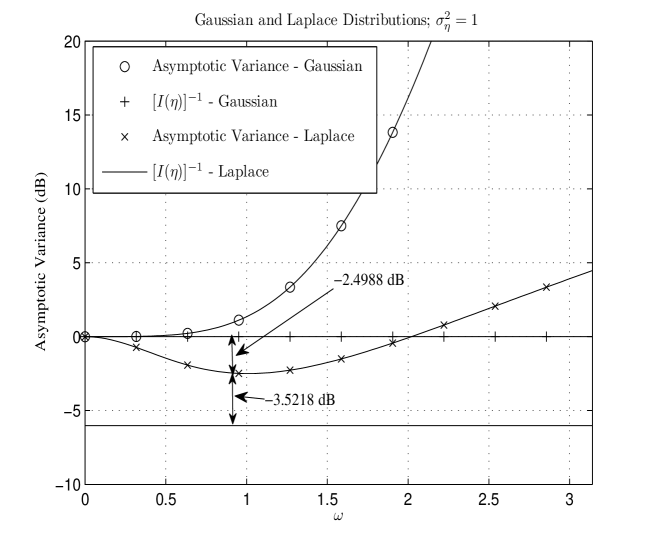
Figure 2: Plot of asymptotic variance vs. $\omega$.

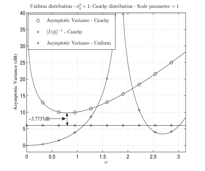
Figure 3: Plot of asymptotic variance vs. $\omega$. Note that the value of $[I(\eta)]^{-1}$ is 0 ($-\infty$ dB) for the uniform sensing noise case and is not shown.

In Figures 2 and 3, the asymptotic variance and the value of $[I(\eta)]^{-1}$ in dB are plotted versus $\omega$, when the sensing noise is Gaussian, Laplace, uniform and Cauchy distributed.

From Figure 2, it can be seen that the asymptotic variance approaches $[I(\eta)]^{-1}$ only as $\omega\to 0$ for Gaussian sensing noise, and is bounded away from $[I(\eta)]^{-1}$ for other values of $\omega$. The estimator in (10) is not efficient when the sensing noise is non-Gaussian. Using the definition of relative efficiency in (24), it can seen from Figure 2 that $\mathcal{E}(\eta)$ in the case of Gaussian sensing noise is $0$dB, and in the case of Laplace sensing noise is about $-3.5$dB. In Figure 2, it can be verified that $\inf_{\omega}\text{AsV}(\omega)\approx 0.75$, which is about $-2.5$dB at $\omega=1/\sqrt{2}$, which is lower than the Gaussian sensing noise case.

From Figure 3 the relative efficiency for the Cauchy noise case is about $-3.8$dB, verifying the value shown in Table I. The inverse Fisher information for the uniform case is 0 ($-\infty$ dB) and is not shown in Figure 3. The relative efficiency as defined in (24), for uniform noise, is therefore zero. When the sensing noise follows the Cauchy, uniform or Laplace distributions, the estimator is not asymptotically efficient.

V Conclusions

In this paper, we considered the relationship between the Fisher information and the characteristic function through two bounds. The condition for equality was also derived, for the first time in literature.

This result was used to prove the asymptotic efficiency of a distributed estimator that minimizes the asymptotic variance in the presence of Gaussian sensing noise. In all cases, the loss in efficiency was quantified through a scale-invariant relative efficiency metric that takes values between 0 and 1. This metric depends only on the distribution of the sensing noise used, and was computed for the Gaussian, Laplace, Cauchy and uniform cases. These relative efficiency values can be interpreted as the amount of information lost due to constant modulus transmissions over Gaussian multiple-access channels relative to having perfect access to all sensor measurements. Numerical evaluations confirm the result that the estimator in (10) is asymptotically efficient only when the sensing noise is Gaussian.

References

• [1] Z.Β Zhang, β€œInequalities for characteristic functions involving Fisher information,” C. R. Acad. Sci. Paris, vol. 344, no.Β 5, pp. 327–330, March 2007.
• [2] T.Β M. Cover and J.Β A. Thomas, Elements of Information Theory.Β Β Β John Wiley and Sons, 1991.
• [3] R.Β Zamir, β€œA proof of the Fisher information inequality via a data processing argument,” Information Theory, IEEE Transactions on, vol.Β 44, no.Β 3, pp. 1246–1250, May 1998.
• [4] O.Β Johnson, Information Theory and the Central Limit Theorem.Β Β Β London: Imperial College Press, 2004.
• [5] E.Β L. Lehmann and G.Β Casella, Theory of Point Estimation.Β Β Β New York: Springer-Verlag, 1998.
• [6] B.Β Porat, Digital processing of random signals: theory and methods.Β Β Β Prentice-Hall, Englewood Cliffs, NJ, 1994.
• [7] A.Β Feuerverger and P.Β McDunnough, β€œOn the efficiency of empirical characteristic function procedures,” Journal of the Royal Statistical Society. Series B (Methodological), vol.Β 43, no.Β 1, pp. 20–27, 1981.
• [8] C.Β Tepedelenlioğlu and A.Β B. Narasimhamurthy, β€œDistributed estimation with constant modulus signals over multiple access channels,” Proceedings of ICASSP 2010, pp. 2290–2293, March 2010.
• [9] R.Β M. Corless, G.Β H. Gonnet, D.Β E.Β G. Hare, D.Β J. Jeffrey, and D.Β E. Knuth, β€œOn the Lambert W function,” Advances in Computational Mathematics, vol.Β 5, pp. 329–359, 1996.