Trispectrum estimator in equilateral type non-Gaussian models

Abstract

We investigate an estimator to measure the primordial trispectrum in equilateral type non-Gaussian models such as k-inflation, single field DBI inflation and multi-field DBI inflation models from Cosmic Microwave Background (CMB) anisotropies. The shape of the trispectrum whose amplitude is not constrained by the bispectrum in the context of effective theory of inflation and k-inflation is known to admit a separable form of the estimator for CMB anisotropies. We show that this shape is $87\%$ correlated with the full quantum trispectrum in single field DBI inflation, while it is $33\%$ correlated with the one in multi-field DBI inflation when curvature perturbation is originated from purely entropic contribution. This suggests that $g_{\rm NL}^{equil}$, the amplitude of this particular shape, provides a reasonable measure of the non-Gaussianity from the trispectrum in equilateral non-Gaussian models. We relate model parameters such as the sound speed, $c_{s}$ and the transfer coefficient from entropy perturbations to the curvature perturbation, $T_{\mathcal{R}S}$ with $g_{\rm NL}^{equil}$, which enables us to constrain model parameters in these models once $g_{\rm NL}^{equil}$ is measured in WMAP and Planck.

I Introduction

The statistical properties of primordial fluctuations provide crucial information on the physics of the very early universe Komatsu:2010fb ; Smith:2009jr ; Senatore:2009gt ; Fergusson:2010dm (See Bartolo:2004if for a review). In the simplest single field inflation models where the scalar field has a canonical kinetic term and quantum fluctuations are generated from the standard Bunch-Davis vacuum, non-Gaussianity of the fluctuations is too small to be observed even with future experiments Acquaviva:2002ud ; Maldacena:2002vr ; Seery:2005wm . Thus the detection of non-negligible departures from Gaussinaity of primordial fluctuations will have a huge impact on the models of early universe. So far, most of the studies have focused on the leading order non-Gaussianity measured by the three-point function of Cosmic Microwave Background (CMB) anisotropies, i.e. the bispectrum Verde:1999ij ; Wang:1999vf ; Komatsu:2001rj . Especially, the optical method of extracting the bispectrum from the CMB data has been sufficiently developed Komatsu:2003iq ; Babich:2004gb ; Babich:2005en ; Creminelli:2005hu ; Creminelli:2006gc ; Yadav:2007rk ; Yadav:2007ny (for a more general approach, see Fergusson:2006pr ; Fergusson:2008ra ; Fergusson:2009nv ). However, future experiments like Planck Planck can also prove the higher order statistics such as the trispectrum Hu:2001fa ; Okamoto:2002ik ; Kogo:2006kh . The trispectrum gives information that cannot be obtained from the bispectrum Seery:2006js ; Seery:2006vu ; Byrnes:2006vq . In addition, it is possible that the trispectrum can be the leading order non-Gaussianity, that is, even if we do not detect the bispectrum, this does not mean that the primordial fluctuations are confirmed to be Gaussian.

In the local type non-Gaussian models Byrnes:2010em ; Langlois:2010vx ; Tanaka:2010km ; Wands:2010af , the primordial curvature perturbation $\zeta$ is modeled as

$$\zeta=\zeta_{g}+\frac{3}{5}f^{local}_{\rm NL}(\zeta_{g}^{2}-\langle\zeta_{g}^{2}\rangle)+\frac{9}{25}g^{local}_{\rm NL}\zeta_{g}^{3}$$ (1)

where $\zeta_{g}$ is a Gaussian variable Sasaki:2006kq . In this model, the bispectrum has maximum amplitude for the squeezed configurations in the Fourie space where one of wavenumbers is small compared with others. In these models, the trispectrum indeed gives very interesting tests on multi-field inflation models where there are several Gaussian variables $\zeta_{g}$ using the consistency relation between the amplitudes of the bispectrum and trispectrum Suyama:2007bg . Also the trispectrum can constrain the cubic-order non-linearities in primordial curvature perturbation, $g^{local}_{\rm NL}$ that cannot be constrained by the bispectrum measurements. Estimators to measure the trispectrum in the local-type non-Gaussianity have been developed and the kurtosis based estimator Munshi:2009wy have been used to obtain constraints on the amplitude of the trispectrum, $-7.4<g_{\rm NL}^{local}/10^{5}<8.2$ at $95\%$ confidence level from the WMAP 5-year data Smidt:2010sv .

There are another class of non-Gaussian models. A typical example is Dirac-Born-Infled (DBI) inflation Silverstein:2003hf whose non-Gaussian property was extensively studied by Alishahiha:2004eh ; Chen:2004gc ; Chen:2005ad ; Chen:2005fe ; Shandera:2006ax ; Chen:2006nt ; Langlois:2008wt ; Langlois:2008qf ; Arroja:2008yy ; Khoury:2008wj ; Langlois:2009ej ; Cai:2009hw (see also Koyama:2010xj ; Chen:2010xk for reviews). In this model, like k-inflation ArmendarizPicon:1999rj ; Garriga:1999vw , the inflaton field has non-canonical kinetic term and non-linear derivative interactions can give rise to large non-Gaussianity of quantum fluctuations. For current observational constraints on DBI inflation see Kecskemeti:2006cg ; Lidsey:2006ia ; Baumann:2006cd ; Bean:2007hc ; Lidsey:2007gq ; Peiris:2007gz ; Kobayashi:2007hm ; Easson:2007dh ; Lorenz:2007ze ; Bean:2007eh ; Bird:2009pq ; Bessada:2009pe ; Copeland:2010jt . In these models, the amplitude of the bispectrum has a peak typically for the equilateral configuration in the Fourie space. The shape of the trispectrum is more complicated. For example, for the bispectrum, the equilateral condition $k_{1}=k_{2}=k_{3}$ completely specifies the shape of the bisepctrum, but this is not the case for the trispectrum. The shape of the trispectrum has been analyzed in several inflationary models such as single field DBI inflation Huang:2006eh ; Arroja:2008ga ; Arroja:2009pd ; Chen:2009bc , multi-field DBI inflation Gao:2009gd ; Mizuno:2009cv ; Mizuno:2009mv ; RenauxPetel:2009sj ; Gao:2009at and the models motivated by effective theory of inflation Senatore:2010jy ; Bartolo:2010di .

Regardless of these efforts, since the form of the trispectrum is generally very complicated, estimators for the trispectrum in this class of non-Gaussian models have not been implemented yet so far. It was suggested that the form of trispectrum given by

$$T_{\zeta}(k_{1},k_{2},k_{3},k_{4})=\frac{g_{\rm NL}^{equil}}{k_{1}k_{2}k_{3}k_{4}(\frac{k_{1}+k_{2}+k_{3}+k_{4}}{4})^{5}}{\cal P}_{\zeta}(k)^{3}\,,$$ (2)

represents the shape of the trispectrum in equilateral non-Gaussian models very well. Here the trispectrum of the curvature perturbation is defined as

$$\langle\zeta({\bf k}_{1})\zeta({\bf k}_{2})\zeta({\bf k}_{3})\zeta({\bf k}_{4})\rangle=(2\pi)^{3}\delta^{3}({\bf k}_{1}+{\bf k}_{2}+{\bf k}_{3}+{\bf k}_{4})T_{\zeta}(k_{1},k_{2},k_{3},k_{4}),$$ (3)

where ${\cal P}_{\zeta}(k)$ is the power spectrum given by $\langle\zeta({\bf k_{1}})\zeta({\bf k_{2}})\rangle=(2\pi)^{3}\delta^{(3)}({\bf k_{1}}+{\bf k_{2}})k_{1}^{-3}{\cal P}_{\zeta}(k_{1})$. This trispectrum (2) appears in DBI inflation as a contribution from the fourth order interacting Hamiltonian (the “contact interaction”) Arroja:2009pd ; Chen:2009bc . In the effective theory of inflation, it was shown that the trispectrum of this shape can have the amplitude that is not constrained by the bispectrum measurements Senatore:2010jy . In Ref. Chen:2009bc , it was suggested that this trispectrum can be used to construct an estimator because by introducing the integral $1/M^{n}=(1/\Gamma(n))\int^{\infty}_{0}t^{(n-1)}e^{-Mt}$, this function is factorisable (see Appendix A). Therefore, in this paper, we compare the shapes of trispectra in single field and multi-field DBI inflation with Eq. (2) based on a shape correlator introduced by Regan et.al Regan:2010cn and investigate whether the estimator constructed from the trispectrum (2) represents the shapes of trispetrum in these models or not.

This paper is organized as follows. In section II, we review the shape correlator introduced by Regan et al. Regan:2010cn . In section III, we study the overlap between the shape given by Eq. (2) and trispectra in single field and multi-field DBI inflation models. In section IV, we give theoretical predictions for $g_{\rm NL}^{equil}$ in some concrete theoretical models. We conclude in section V. In Appendix A, we present the optimal estimator using Eq. (2) explicitly. In Appendix B, we summarise the shape function of the reduced trispectra appeared in general single field k-inflation models and give the shape correlations among the representative shapes. In Appendix C, we check the validity of our method to relate the amplitude of the estimator to the theoretical predictions using the bispectrum.

II The shape correlator

In this section, we review the shape correlator introduced by Regan et al. Regan:2010cn .

II.1 Shape functions

First we exploit the symmetry of the trispectrum to define the reduced trispectrum as follows Hu:2001fa . We rewrite the definition of the trispectrum as

$$\langle\zeta({\bf k_{1}})\zeta({\bf k_{2}})\zeta({\bf k_{3}})\zeta({\bf k_{4}})\rangle_{c} = (2\pi)^{3}\int d^{3}K\bigl{[}\delta({\bf k_{1}}+{\bf k_{2}}-{\bf K})\delta({\bf k_{3}}+{\bf k_{4}}+{\bf K})\bigl{(}\mathcal{T}_{\zeta}({\bf k_{1}},{\bf k_{2}},{\bf k_{3}},{\bf k_{4}};{\bf K})$$ (4)

$$+\mathcal{T}_{\zeta}({\bf k_{2}},{\bf k_{1}},{\bf k_{3}},{\bf k_{4}};{\bf K})+\mathcal{T}_{\zeta}({\bf k_{1}},{\bf k_{2}},{\bf k_{4}},{\bf k_{3}};{\bf K})+\mathcal{T}_{\zeta}({\bf k_{2}},{\bf k_{1}},{\bf k_{4}},{\bf k_{3}};{\bf K})\bigr{)}$$

$$+({\bf k_{2}}\leftrightarrow{\bf k_{3}})+({\bf k_{2}}\leftrightarrow{\bf k_{4}})\bigr{]}\,.$$

Then we need to consider only the reduced trispectrum $\mathcal{T}_{\zeta}$ from one particular arrangement of the vectors, such as $\mathcal{T}_{\Phi}({\bf k_{1}},{\bf k_{2}},{\bf k_{3}},{\bf k_{4}};{\bf k_{12}})$ with ${\bf k_{12}}={\bf k_{1}}+{\bf k_{2}}$ and form the other contributions by considering permutations. Here, for the later convenience, we use the symmetrised reduced trispectrum

$$\mathcal{T}_{\zeta}^{sym}({\bf k_{1}},{\bf k_{2}},{\bf k_{3}},{\bf k_{4}};{\bf k_{12}}) \equiv \frac{1}{4}\bigl{[}\mathcal{T}_{\zeta}({\bf k_{1}},{\bf k_{2}},{\bf k_{3}},{\bf k_{4}};{\bf k_{12}})+\mathcal{T}_{\zeta}({\bf k_{2}},{\bf k_{1}},{\bf k_{3}},{\bf k_{4}};{\bf k_{12}})$$ (5)

$$+\mathcal{T}_{\zeta}({\bf k_{1}},{\bf k_{2}},{\bf k_{4}},{\bf k_{3}};{\bf k_{12}})+\mathcal{T}_{\zeta}({\bf k_{2}},{\bf k_{1}},{\bf k_{4}},{\bf k_{3}};{\bf k_{12}})\bigr{]}\,,$$

and from now on we omit the superscript $sym$ for simplicity.

The reduced trispectrum is a function of six variables. We can choose them to be $(k_{1},k_{2},k_{3},k_{4},k_{12},\theta_{4})$ where $\theta_{4}$ represents the deviation of the quadrilateral from planarity which is specified by the triangle $(k_{1},k_{2},k_{12})$. We find that in terms of these variables $k_{14}=|{\bf k_{1}}+{\bf k_{4}}|$ is expressed as

$$k_{14}^{2} = k_{1}^{2}+k_{4}^{2}-\frac{1}{2k_{12}^{2}}(k_{1}^{2}+k_{12}^{2}-k_{2}^{2})(k_{4}^{2}+k_{12}^{2}-k_{3}^{2})$$ (6)

$$\pm\frac{1}{2k_{12}^{2}}\sqrt{4k_{1}^{2}k_{12}^{2}-(k_{1}^{2}+k_{12}^{2}-k_{2}^{2})^{2}}\sqrt{4k_{4}^{2}k_{12}^{2}\cos^{2}\theta_{4}-(k_{4}^{2}+k_{12}^{2}-k_{3}^{2})^{2}}\,,$$

which implies that the valid range of $\cos\theta_{4}$ is constrained by

$$|\cos\theta_{4}|\geq\frac{|k_{4}^{2}+k_{12}^{2}-k_{3}^{2}|}{2k_{12}k_{4}}\,.$$ (7)

Motivated by the relation between the CMB trispectrum and the trispectrum for $\zeta$, the shape function for the reduced trispectrum is defined as

$$S_{\mathcal{T}}(k_{1},k_{2},k_{3},k_{4},k_{12},\theta_{4})=(k_{1}k_{2}k_{3}k_{4})^{2}k_{12}\mathcal{T}_{\zeta}(k_{1},k_{2},k_{3},k_{4};k_{12},\theta_{4})\,.$$ (8)

Regan et al. Regan:2010cn proposed to define an overlap between two different shape functions $S_{\mathcal{T}}$ and $S_{\mathcal{T}^{\prime}}$ as

$$F(S_{\mathcal{T}},S_{\mathcal{T}^{\prime}})=\int d\mathcal{V}_{k}\int d(\cos\theta_{4})S_{\mathcal{T}}(k_{1},k_{2},k_{3},k_{4},k_{12},\theta_{4})S_{\mathcal{T}^{\prime}}(k_{1},k_{2},k_{3},k_{4},k_{12},\theta_{4})w(k_{1},k_{2},k_{3},k_{4},k_{12})\,,$$ (9)

where $w$ is an appropriate weight function. The weight function should be chosen such that $S^{2}w$ in $k$ space produces the same scaling as the estimator in $l$ space and we adopt the one used in Ref. Regan:2010cn ,

$$w(k_{1},k_{2},k_{3},k_{4},k_{12})=\frac{1}{k_{12}(k_{1}+k_{2}+k_{12})(k_{3}+k_{4}+k_{12})}\,.$$ (10)

With this choice of weight, the shape correlator is defined as

$$\bar{\mathcal{C}}(S_{\mathcal{T}},S_{\mathcal{T}^{\prime}})=\frac{F(S_{\mathcal{T}},S_{\mathcal{T}^{\prime}})}{\sqrt{F(S_{\mathcal{T}},S_{\mathcal{T}})F(S_{\mathcal{T}^{\prime}},S_{\mathcal{T}^{\prime}})}}\,.$$ (11)

II.2 Parameterisation of six parameters

First to parameterise the magnitude of the momenta, we use the semiperimeter of the triangle formed by the vectors ${\bf k}_{1},{\bf k}_{2},{\bf k}_{1}+{\bf k}_{2}$,

$$q\equiv\frac{1}{2}(k_{1}+k_{2}+k_{12})\,.$$ (12)

From the scaling behaviour, the form of the shape function on a constant-$q$ cross section becomes independent of $q$ and we can write

$$S_{\mathcal{T}}(k_{1},k_{2},k_{3},k_{4},k_{12},\theta_{4})=f(q)\bar{S}_{\mathcal{T}}(\hat{k}_{1},\hat{k}_{2},\hat{k}_{3},\hat{k}_{4},\hat{k}_{12},\theta_{4})\,,$$ (13)

where $\hat{k}_{i}\equiv k_{i}/q$ and $\hat{k}_{12}=k_{12}/q$. Since we are restricted to the region where the momenta $(k_{1},k_{2},k_{12})$ and $(k_{3},k_{4},k_{12})$ form triangles by momentum conservation, we will reparameterise the allowed region to separate out the overall scale $q$ from the behaviour on a constant $q$ cross-sectional slice. This five-dimensional slice is spanned by the remaining coordinates. For triangle $(k_{1},k_{2},k_{12})$ we have

$$k_{12} = q(1-\beta)\,,$$ (14)

$$k_{1} = \frac{q}{2}(1+\alpha+\beta)\,,$$ (15)

$$k_{2} = \frac{q}{2}(1-\alpha+\beta)\,,$$ (16)

while for triangle $(k_{3},k_{4},k_{12})$

$$k_{12} = \epsilon q(1-\delta)\,,$$ (17)

$$k_{3} = \frac{\epsilon q}{2}(1+\gamma+\delta)\,,$$ (18)

$$k_{4} = \frac{\epsilon q}{2}(1-\gamma+\delta)\,,$$ (19)

where $\epsilon$ parameterises the ratio of the perimeters of the two triangles, i.e. $\epsilon=(k_{3}+k_{4}+k_{12})/(k_{1}+k_{2}+k_{12})$. We do not lose the generality to consider $1\leq\epsilon<\infty$. The different expressions for $k_{12}$ imply that

$$1-\beta=\epsilon(1-\delta)\,,$$ (20)

from which $\delta$ is eliminated to give

$$k_{3} = \frac{q}{2}(-1+\beta+(2+\gamma)\epsilon)\,,$$ (21)

$$k_{4} = \frac{q}{2}(-1+\beta+(2-\gamma)\epsilon)\,.$$ (22)

The conditions for triangle $(k_{1},k_{2},k_{12})$ that $0\leq k_{1},k_{2},k_{12}\leq q$ imply that $0\leq\beta\leq 1$ and $-(1-\beta)\leq\alpha\leq 1-\beta$, while the condition for triangle $(k_{3},k_{4},k_{12})$ that $0\leq k_{3},k_{4},k_{12}\leq\epsilon k_{12}$ imply that $-(1-\beta)/\epsilon\leq\gamma\leq(1-\beta)/\epsilon$. Furthermore, in terms of these variables, the condition (7) is expressed as

$$|\cos\theta_{4}|\geq\frac{|1+\beta^{2}-\gamma\epsilon(-1+2\epsilon)-\beta(2+\gamma\epsilon)|}{(1-\beta)(-1+\beta+(2-\gamma)\epsilon)}\,.$$ (23)

In summary, we have the following domains,

$$0\leq q<\infty,\;\;1\leq\epsilon<\infty\,,\;\;0\leq\beta\leq 1\,,\;\;-(1-\beta)\leq\alpha\leq 1-\beta,\;\;-\frac{1-\beta}{\epsilon}\leq\gamma\leq\frac{1-\beta}{\epsilon}\,,$$ (24)

together with Eq. (23). In practice, we introduce a cutoff for the integration of $\epsilon$ as $S_{\mathcal{T}}S_{\mathcal{T}}w$ is decreasing with $\epsilon$ asymptotically after integrating out the dependence of $\alpha$, $\gamma$ and $\beta$ in the overlap integral. we set the cut-off to be $\epsilon=10$ but the dependence on this cut-off is very weak. Also we should emphasize that the CMB measurements will never prove the parameter region where $\epsilon\gg 1$.

Making use of this parameterisation, the shape function (13), the weight function (10) and the volume element can be rewritten as

$$S_{\mathcal{T}}(k_{1},k_{2},k_{3},k_{4},k_{12},\theta_{4}) = f(q)\bar{S}_{\mathcal{T}}(\alpha,\beta,\gamma,\epsilon,\theta_{4})\,,$$

$$w(k_{1},k_{2},k_{3},k_{4},k_{12}) = \frac{1}{4\epsilon(1-\beta)}\,,$$ (25)

$$d\mathcal{V}_{k}=dk_{1}dk_{2}dk_{3}dk_{4}dK = \epsilon q^{4}dqd\alpha d\beta d\gamma d\epsilon\,.$$ (26)

It is worth noting that although the integration $d\mathcal{V}_{k}$ is five-dimensional in Eq. (9), for scale-invariant shape functions with constant $f(q)$, it is enough to evaluate shape correlations only for the four dimensional slices with constant $q$.

III Shape correlations

In this section, we study the overlap between Eq. (2) and the trispectra in single field and multi-field DBI inflation. It is worth mentioning that from the definition of the shape correlator (11), the shape correlations are independent of the normalisations of shape functions. We will discuss the normalisation of the trispectrum in the next section.

III.1 Equilateral shape

First, we find that the shape function for the trispectrum (2) is given by

$$S_{\mathcal{T}}^{equil} = N^{equil}S_{\mathcal{T}}^{c_{1}}\,,$$ (27)

$$N^{equil} = \frac{64}{3}{\cal P}_{\zeta}^{3}g_{\rm NL}^{equil}\,,$$ (28)

where $S_{\mathcal{T}}^{c_{1}}$ is given by Eq. (71). We will assume the scale independence of the spectrum ${\cal P}_{\zeta}$ in the rest of the paper. In k-inflation model, this class of models are characterised by $P_{,4X}\gg X^{-2}P_{,XX},X^{-1}P_{,XXX}$ for the action given by Eq. (63). It was also shown that, in the context of the effective theory of inflation, it is possible to construct consistent inflationary models where the trispectrum is characterised by this shape function and its amplitude is not constrained by the bispectrum Senatore:2010jy .

As this shape function depends on $\alpha$, $\beta$, $\gamma$, $\epsilon$, first, we clarify the $\epsilon$ dependence of the signal which is given by $S_{\mathcal{T}}^{equil}S_{\mathcal{T}}^{equil}w$. We find that after integrating out the dependence of $\alpha$, $\beta$ and $\gamma$ in the overlap integration, the amplitude of the signal is proportional to $1/\epsilon^{7}$ asymptotically. This shows that the dominant contribution to the signal for this shape is coming from $\epsilon\sim 1$. In Fig. 1, we show the $\epsilon$ dependence of $S_{\mathcal{T}}^{equil}S_{\mathcal{T}}^{equil}w$.

Figure 1: We show the $\epsilon$ dependence of $S_{\mathcal{T}}^{equil}S_{\mathcal{T}}^{equil}w$ (solid line), $S_{\mathcal{T}}^{DBI(\sigma)}S_{\mathcal{T}}^{equil}w$ (dashed line) and $S_{\mathcal{T}}^{DBI(s)}S_{\mathcal{T}}^{equil}w$ (dotted line) by integrating out the dependence of $\alpha$, $\beta$ and $\gamma$ in the overlap integration. We find that $S_{\mathcal{T}}^{DBI(\sigma)}S_{\mathcal{T}}^{equil}w$ and $S_{\mathcal{T}}^{DBI(s)}S_{\mathcal{T}}^{equil}w$ asymptote to $\propto 1/\epsilon^{4}$ while $S_{\mathcal{T}}^{equil}S_{\mathcal{T}}^{equil}w$ $\propto 1/\epsilon^{7}$ for large $\epsilon$. We find that while $S_{\mathcal{T}}^{DBI(\sigma)}S_{\mathcal{T}}^{equil}w$ is always positive, $S_{\mathcal{T}}^{DBI(s)}S_{\mathcal{T}}^{equil}w$ become negative above some critical value of $\epsilon$. Because of this, the full overlap between $S^{DBI(s)}_{\mathcal{T}}$ and $S^{equil}_{\mathcal{T}}$ takes much smaller value than the one estimated at configurations with $\epsilon=1$. We have normalised so that the values become $1$ at $\epsilon=1$.

Next, we examine the $\alpha$, $\beta$, $\gamma$ dependence of $S_{\mathcal{T}}^{equil}$. For this purpose, we plot $S_{\mathcal{T}}^{equil}(\alpha,\beta,\gamma,\epsilon)$ evaluated at $\epsilon=1$ for given $\beta$ in Fig. 2 where $S_{\mathcal{T}}^{equil}$ is symmetric under the exchange of $\alpha$ and $\gamma$ for the configurations with $\epsilon=1$ and the physical region is given by $1-\beta>\alpha,\gamma>\beta-1$.

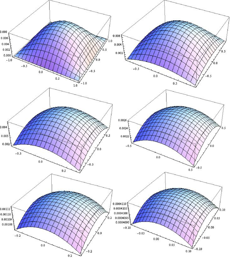
Figure 2: In this group of figures, we plot $S_{\mathcal{T}}^{equil}(\alpha,\beta,\gamma,\epsilon)$ with $\epsilon=1$. $\beta=0,0.1,0.25,0.5,0.75,0.9$ for upper left, upper right, middle left, middle right, lower left, lower right, respectively. Vertical axes for each plot denote $\alpha$ and $\gamma$. For these configurations, $S_{\mathcal{T}}^{equil}$ is symmetric under the exchange of $\alpha$ and $\gamma$ and the physical region is given by $1-\beta>\alpha,\gamma>\beta-1$. We set $N^{equil}=1$.

III.2 Single filed DBI inflation

It was suggested in Arroja:2009pd that the shape function corresponding to the reduced trispectrum of single field DBI inflation at leading order in the slow-roll expansion is given by

$$S^{DBI(\sigma)}_{\mathcal{T}} = N^{DBI(\sigma)}\left[-3S^{c_{1}}_{\mathcal{T}}+\frac{1}{64}S^{s_{1}}_{\mathcal{T}}+\frac{1}{64}S^{s_{2}}_{\mathcal{T}}-\frac{1}{64}S^{s_{3}}_{\mathcal{T}}\right]\,,$$ (29)

$$N^{DBI(\sigma)} = \frac{H^{12}}{\dot{\phi}^{6}c_{s}^{4}}\,,$$ (30)

where $S^{s_{1}}_{\mathcal{T}}$, $S^{s_{2}}_{\mathcal{T}}$ and $S^{s_{3}}_{\mathcal{T}}$ are given by Eqs. (74), (75) and (80), respectively.

Similar to the case of the equilateral shape, first we examine the $\epsilon$ dependence. In Fig. 1, we plot $S_{\mathcal{T}}^{DBI(\sigma)}S_{\mathcal{T}}^{equil}w$. We find that after integrating out the dependence of $\alpha$, $\beta$ and $\gamma$ in the overlap integration, the amplitude of the signal is proportional to $1/\epsilon^{4}$ asymptotically. This shows that the dominant contribution to the overlap between the single field DBI model and the equilateral shape is coming from $\epsilon\sim 1$. The difference of the asymptotic $\epsilon$ dependence between the trispectra corresponding to the differences of the shapes between $S_{\mathcal{T}}^{c_{1}}$, which is coming from the contact interaction and $S_{\mathcal{T}}^{s_{1}}$, $S_{\mathcal{T}}^{s_{2}}$, $S_{\mathcal{T}}^{s_{3}}$, which arise from the scalar exchanges. This was pointed out in Ref. Chen:2009bc by considering the double squeezed limit ($k_{3}=k_{4}=k_{12}\to 0$). Therefore, it is natural that the asymptotic $\epsilon$ dependence between $S_{\mathcal{T}}^{equil}$ and $S_{\mathcal{T}}^{DBI(\sigma)}$ is different, as $S_{\mathcal{T}}^{DBI(\sigma)}$ is obtained by a linear combination of $S_{\mathcal{T}}^{s_{1}}$, $S_{\mathcal{T}}^{s_{2}}$ and $S_{\mathcal{T}}^{s_{3}}$.

Next, we examine the $\alpha$, $\beta$, $\gamma$ dependence of $S_{\mathcal{T}}^{DBI(\sigma)}$. For this purpose, we plot $S_{\mathcal{T}}^{DBI(\sigma)}(\alpha,\beta,\gamma,\epsilon)$ evaluated at $\epsilon=1$ for given $\beta$ in Fig. 3 where $S_{\mathcal{T}}^{DBI(\sigma)}$ is symmetric under the exchange of $\alpha$ and $\gamma$ for the configurations with $\epsilon=1$ and the physical region is given by $1-\beta>\alpha,\gamma>\beta-1$.

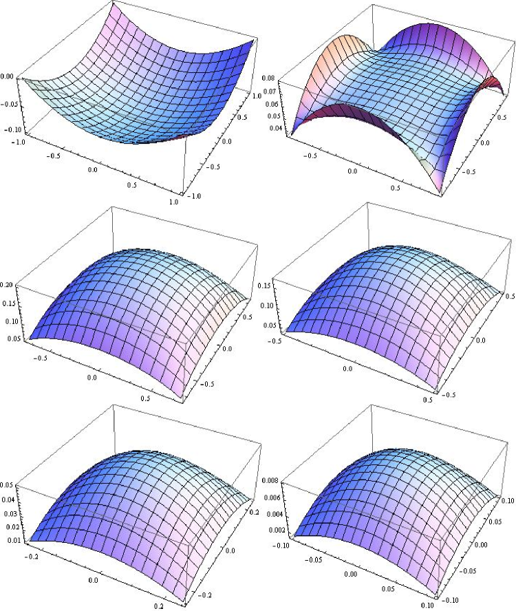
Figure 3: In this group of figures, we plot $S_{\mathcal{T}}^{DBI(\sigma)}(\alpha,\gamma,\beta)$ with $\epsilon=1$. $\beta=0,0.1,0.25,0.5,0.75,0.9$ for upper left, upper right, middle left, middle right, lower left, lower right, respectively. Vertical axes for each plot denote $\alpha$ and $\gamma$. For these configurations, $S_{\mathcal{T}}^{DBI(\sigma)}$ is symmetric under the exchange of $\alpha$ and $\gamma$ and the physical region is given by $1-\beta>\alpha,\gamma>\beta-1$. We set $N^{DBI(\sigma)}=1$.

Except for the region with very small value of $\beta$ (from $0$ to $\sim 0.1$) the shapes are very similar to $S_{\mathcal{T}}^{equil}$. This explains that the overlap between $S_{\mathcal{T}}^{DBI(\sigma)}$ and $S_{\mathcal{T}}^{equil}$ is sufficiently large for the configurations with $\epsilon=1$.

Table 1 provides a summary of correlations between $S_{\mathcal{T}}^{equil}$ and $S_{\mathcal{T}}^{DBI(\sigma)}$. In addition to the correlation considering full configurations dealing with five dimensional parameter space, for comparisons, we also consider the configurations limited with $\epsilon=1$ and equilateral configurations ($\epsilon=1$, $\alpha=\gamma=0$). The overlap decrease if we include the non-equilateral configurations keeping $\epsilon=1$. This is due to the difference of the shapes for small $\beta$. Also the different asymptotic behaviours with respect to $\epsilon$ further reduces the overlap if we integrate over $\epsilon$. However, even after we perform the all integration, the overlap remains high at around 87$\%$ level.

III.3 Multi-field DBI inflation

It was suggested in Mizuno:2009mv that the reduced trispectrum of multi-field DBI inflation dominated by originally purely entropic perturbations at leading order in the slow-roll expansion is given by

$$S^{DBI(s)}_{\mathcal{T}} = N^{DBI(s)}\left[-\frac{1}{8}S^{c_{2}}_{\mathcal{T}}+\frac{1}{576}S^{s_{1}}_{\mathcal{T}}+\frac{1}{64}S^{\tilde{s}_{2}}_{\mathcal{T}}+\frac{1}{192}S^{\tilde{s}_{3}}_{\mathcal{T}}\right]\,,$$ (31)

$$N^{DBI(s)} = \frac{H^{12}}{\dot{\phi}^{6}c_{s}^{4}}T_{\mathcal{R}S}^{4}\,,$$ (32)

where $S^{\tilde{s}_{2}}_{\mathcal{T}}$ and $S^{\tilde{s}_{3}}_{\mathcal{T}}$ are given by Eqs. (93) and (94), respectively.

Again, we first examine the $\epsilon$ dependence of the overlap (in Fig. 1). We find that after integrating out the dependence of $\alpha$, $\beta$ and $\gamma$, the amplitude of the overlap, $S_{\mathcal{T}}^{equil}S_{\mathcal{T}}^{DBI(s)}w$ is proportional to $1/\epsilon^{4}$ asymptotically as in the single field case. This shows that the dominant contribution to the signal for this shape is coming from $\epsilon\sim 1$.

The asymptotic $\epsilon$ dependence of $S_{\mathcal{T}}^{DBI(s)}$ is the same as that of $S_{\mathcal{T}}^{DBI(\sigma)}$. We find that asymptotically $S_{\mathcal{T}}^{s_{2b}}$, $S_{\mathcal{T}}^{s_{2d}}$ and $S_{\mathcal{T}}^{s_{3b}}$ given by Eqs. (77), (79) and (82) give the dominant contribution to both $S_{\mathcal{T}}^{DBI(\sigma)}$ and $S_{\mathcal{T}}^{DBI(s)}$, which characterises the asymptotic $\epsilon$ dependence. However, as is shown in Fig. 1, $S_{\mathcal{T}}^{DBI(s)}S_{\mathcal{T}}^{equil}w$ become negative above some critical value of $\epsilon$. This reduces the final overlap once we integrate over $\epsilon$.

Next, we examine the $\alpha$, $\beta$, $\gamma$ dependence of $S_{\mathcal{T}}^{DBI(s)}$. For this purpose, again we plot $S_{\mathcal{T}}^{DBI(s)}(\alpha,\beta,\gamma,\epsilon)$ evaluated at $\epsilon=1$ for given $\beta$ in Fig. 4 where $S_{\mathcal{T}}^{DBI(s)}$ is symmetric under the exchange of $\alpha$ and $\gamma$ for the configurations with $\epsilon=1$ and the physical region is given by $1-\beta>\alpha,\gamma>\beta-1$.

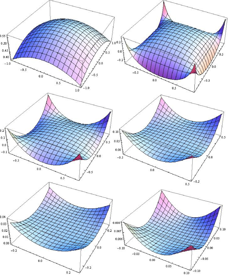
Figure 4: In this group of figures, we plot $S_{\mathcal{T}}^{DBI(s)}(\alpha,\gamma,\beta)$ with $\epsilon=1$. $\beta=0,0.1,0.25,0.5,0.75,0.9$ for upper left, upper right, middle left, middle right, lower left, lower right, respectively. Vertical axes for each plot denote $\alpha$ and $\gamma$. For these configurations, $S_{\mathcal{T}}^{DBI(s)}$ is symmetric under the exchange of $\alpha$ and $\gamma$ and the physical region is given by $1-\beta>\alpha,\gamma>\beta-1$. We set $N^{DBI(s)}=1$.

Except for the region with very small value of $\beta$ (from $0$ to $\sim 0.1$) the shape is different from $S_{\mathcal{T}}^{equil}$. This explains that the overlap between $S_{\mathcal{T}}^{DBI(s)}$ and $S_{\mathcal{T}}^{equil}$ is not so large even for the configurations with $\epsilon=1$.

Table 1 provides a summary of correlations between $S_{\mathcal{T}}^{equil}$ and $S_{\mathcal{T}}^{DBI(s)}$. As in the single field case, in addition to the correlation considering full configurations dealing with five dimensional parameter space, for comparisons, we also consider the configurations limited with $\epsilon=1$ and equilateral configurations ($\epsilon=1$, $\alpha=\gamma=0$).

Table 1 shows that the overlap becomes smaller once we include the non-equilateral configurations with $\epsilon=1$. This is clear from the shape difference for $\beta>0.1$. In addition the shape correlation for full configurations becomes further smaller once we integrate over $\epsilon$. As explained before, this is due to the fact that while $S_{\mathcal{T}}^{DBI(\sigma)}S_{\mathcal{T}}^{equil}w$ is always positive, $S_{\mathcal{T}}^{DBI(s)}S_{\mathcal{T}}^{equil}w$ become negative above some critical value of $\epsilon$. This confirms the fact that the shape dependence of trispectrum can in principle distinguish multi-field DBI inflation models form single field DBI inflation models shown by Refs. Mizuno:2009cv ; Mizuno:2009mv . In practice, the overlap still remains at 33$\%$ level after integrating over all the shape parameters and the equilateral shape could still be used to get a reasonable estimation for the constraints on multi-field DBI inflation model.

IV Theoretical predictions for $g_{\rm NL}^{equil}$

In this section, making use of the shape correlations investigated in the previous section, we give theoretical predictions for $g_{\rm NL}^{equil}$. As a consistency check, we applied the same method to estimate the amplitude of the bispectrum in DBI inflation in Appendix C.

In k-inflation models, as is shown in Appendix B by setting $P_{,4X}\gg X^{-2}P_{,XXX},X^{-1}P_{,XXX}$, the shape function is given by

$$S^{equil}_{\mathcal{T}}=\frac{H^{12}P_{,4X}}{16P_{,X}^{4}c_{s}}S^{c_{1}}_{\mathcal{T}}\,.$$ (33)

Then, by comparing Eqs. (27) with (33), we find $g_{\rm NL}^{equil}$ is obtained as

$$g_{\rm NL}^{equil}=\frac{3X^{3}c_{s}^{2}P_{,4X}}{16P_{,X}}\,,$$ (34)

where we have used ${\cal P}_{\zeta}=H^{4}/(4Xc_{s}P_{,X})$ for single field k-inflation.

In order to express the amplitude of trispectrum in single field DBI inflation in terms of $g_{\rm NL}^{equil}$, we rewrite Eq. (29) in the following form:

$$S^{DBI(\sigma)}_{\mathcal{T}} = 0.41{\cal P}_{\zeta}^{3}\frac{g_{\rm NL}^{equil}}{\bar{\mathcal{C}}(S^{DBI(\sigma)}_{\mathcal{T}},S^{equil}_{\mathcal{T}})}\left[-3S^{c_{1}}_{\mathcal{T}}+\frac{1}{64}S^{s_{1}}_{\mathcal{T}}+\frac{1}{64}S^{s_{2}}_{\mathcal{T}}-\frac{1}{64}S^{s_{3}}_{\mathcal{T}}\right]\,,$$ (35)

where the numerical factor in Eq. (35) is chosen so that when $g_{\rm NL}^{equil}=1$ and $\bar{\mathcal{C}}(S^{DBI(\sigma)}_{\mathcal{T}},S^{equil}_{\mathcal{T}})=1$, the following conditions are satisfied,

$$F(S^{DBI(\sigma)}_{\mathcal{T}},S^{DBI(\sigma)}_{\mathcal{T}}) = F(S^{equil}_{\mathcal{T}},S^{equil}_{\mathcal{T}})\,,$$

$$F(S^{DBI(\sigma)}_{\mathcal{T}},S^{equil}_{\mathcal{T}}) > 0\,.$$ (36)

Of course, $\bar{\mathcal{C}}(S^{DBI(\sigma)}_{\mathcal{T}},S^{equil}_{\mathcal{T}})=1$ is not true in reality and this factor will enhance the amplitude of the signal for a given $g_{\rm NL}^{equil}$. This term is necessary because when we use the estimator related with $S^{equil}_{\mathcal{T}}$ for the signal whose shape is characterised by $S^{DBI(\sigma)}_{\mathcal{T}}$, the observed signal is suppressed by $\bar{\mathcal{C}}(S^{DBI(\sigma)}_{\mathcal{T}},S^{equil}_{\mathcal{T}})$ and it is necessary to compensate this. Then, by comparing Eqs. (29) with (36), we can relate $g_{\rm NL}^{equil}$ with the sound speed $c_{s}^{2}$ as

$$g_{NL}^{equil}=\frac{17}{c_{s}^{4}}\,,$$ (37)

where we have used ${\cal P}_{\Phi}=H^{4}/(2\dot{\phi}^{2})$ for single field DBI inflation.

Similarly, in order to express the amplitude of trispectrum in multi-field DBI inflation in terms of $g_{\rm NL}^{equil}$, we rewrite Eq. (31) in the following form:

$$S^{DBI(s)}_{\mathcal{T}} = 1.2{\cal P}_{\zeta}^{3}\frac{g_{\rm NL}^{equil}}{\bar{\mathcal{C}}(S^{DBI(s)}_{\mathcal{T}},S^{equil}_{\mathcal{T}})}\left[-\frac{1}{8}S^{c_{2}}_{\mathcal{T}}+\frac{1}{576}S^{s_{1}}_{\mathcal{T}}+\frac{1}{64}S^{\tilde{s}_{2}}_{\mathcal{T}}+\frac{1}{192}S^{\tilde{s}_{3}}_{\mathcal{T}}\right]\,,$$ (38)

where the numerical factor in Eq. (38) is again chosen so that when $g_{\rm NL}^{equil}=1$ and $\bar{\mathcal{C}}(S^{DBI(s)}_{\mathcal{T}},S^{equil}_{\mathcal{T}})=1$, the following conditions are satisfied,

$$F(S^{DBI(s)}_{\mathcal{T}},S^{DBI(s)}_{\mathcal{T}}) = F(S^{equil}_{\mathcal{T}},S^{equil}_{\mathcal{T}})\,,$$

$$F(S^{DBI(s)}_{\mathcal{T}},S^{equil}_{\mathcal{T}}) > 0\,.$$ (39)

Then, by comparing Eqs. (31) with (39), we can relate $g_{\rm NL}^{equil}$ with the sound speed $c_{s}^{2}$ and the transfer coefficient that relate the amplitude of original entropy perturbations to the final curvature perturbation $T_{\mathcal{R}S}^{2}$ as

$$g_{NL}^{equil}=\frac{2.2}{c_{s}^{4}T_{\mathcal{R}S}^{2}}\,,$$ (40)

where we have used ${\cal P}_{\zeta}=H^{4}T_{\mathcal{R}S}^{2}/(2\dot{\phi}^{2})$ for multi field DBI inflation.

In Table 1, we summarise theoretical predictions for $g^{equil}_{\rm NL}$ for the models discussed in this section.

	Overlap-full	$\epsilon=1$	equilateral	theoretical prediction for $g^{equil}_{\rm NL}$	$f^{equil}_{\rm NL}$
equilateral shape	$1$	$1$	$1$	$(3X^{3}c_{s}^{2}P_{,4X})/(16P_{,X})$	$f^{equil}_{\rm NL}$
single DBI	$0.87$	$0.90$	$0.92$	$17/c_{s}^{4}$	$-0.36/c_{s}^{2}$
multi DBI	$0.33$	$0.60$	$0.85$	$2.2/(c_{s}^{4}T_{\mathcal{R}S}^{2})$	$-0.36/(c_{s}^{2}T_{\mathcal{R}S}^{2})$

Table 1: Shape correlations against $S_{\mathcal{T}}^{equil}$ for full configurations, the configurations restricted to $\epsilon=1$, equilateral configurations ($\epsilon=1$, $\alpha=\gamma=0$) in the model with equilateral shape motivated by effective theory of inflation, single field DBI inflation and multi-field DBI inflation. We also summarise theoretical predictions for $g^{equil}_{\rm NL}$ and $f_{\rm NL}^{equil}$ in these models.

It is instructive to compare the values (37) and (40) with previous results of $\tau_{\rm NL}$ Mizuno:2009mv based on the matching of the amplitude at a specific equilateral configuration. We define the non-linear parameter

$$\tau_{\rm NL}=\frac{T_{\zeta}({\bf k}_{1},{\bf k}_{2},{\bf k}_{3},{\bf k}_{4})k_{1}^{3}k_{2}^{3}k_{3}^{3}k_{4}^{3}{\cal P}_{\zeta}^{-3}}{[(k_{1}^{3}k_{2}^{3}+k_{3}^{3}k_{4}^{3})(k_{13}^{-3}+k_{14}^{-3})+(k_{1}^{3}k_{4}^{3}+k_{2}^{3}k_{3}^{3})(k_{12}^{-3}+k_{13}^{-3})+(k_{1}^{3}k_{3}^{3}+k_{2}^{3}k_{4}^{3})(k_{12}^{-3}+k_{14}^{-3}]},$$ (41)

and evaluated it for the configuration specified by $k_{1}=k_{2}=k_{3}=k_{4}=k$, $k_{12}=k_{13}=k_{14}=(2/\sqrt{3})k$. For single field and multi-field DBI inflation models, we obtain

$$\tau_{\rm NL} = \frac{0.56}{c_{s}^{4}}\,,\;\;{\rm for\;\;single\;\;field\;\;DBI\;\;inflation}$$ (42)

$$\tau_{\rm NL} = \frac{0.12}{c_{s}^{4}T_{\mathcal{R}S}^{2}}\,,\;\;{\rm for\;\;multifield\;\;DBI\;\;inflation}$$ (43)

Using the same procedure, we get $\tau_{\rm NL}=2g_{\rm NL}^{equil}/9\sqrt{3}$. By comparing this to (42) and (43) we can estimate $g_{\rm NL}^{equil}$ as

$$g_{\rm NL}^{equil} = \frac{4.4}{c_{s}^{4}}\,,\;\;{\rm for\;\;single\;\;field\;\;DBI\;\;inflation}$$ (44)

$$g_{\rm NL}^{equil} = \frac{0.94}{c_{s}^{4}T_{\mathcal{R}S}^{2}}\,,\;\;{\rm for\;\;multifield\;\;DBI\;\;inflation}$$ (45)

which underestimates the amplitude by factor $2\sim 4$ compared with the results of Eqs. (37) and (40). This demonstrates that unlike the bispectrum case where the matching of the amplitude at the equilateral configuration gives a reasonable estimation for $f_{\rm NL}^{equil}$, it is necessary to calculate the overlap between the shapes in full five-dimensional parameter space to extract the amplitude of the trispectrum $g_{\rm NL}^{equil}$.

V Conclusion

It is well known that there are many interesting early universe models that predict equilateral type primordial non-Gaussianity motivated by string theory and effective field theory. Taking into account the fact that future experiments such as Planck can prove even next order statistics, it is important to study the primordial trispectrum in these models. For example, we had shown previously that the trispectrum can in principle distinguish multi-field DBI inflation models from single field DBI inflation models from the shape dependence Arroja:2009pd ; Mizuno:2009cv ; Mizuno:2009mv . On the other hand, at the practical level, since the form of the trispectrum is too complicated, the estimator in this class of models had not been implemented explicitly.

Therefore, in this work we have presented a method to estimate primordial trispectrum in equilateral type non-Gaussian models such as k-inflation model whose action is given by Eq. (63), single field DBI inflation and multi-field DBI inflation. Our method is based on the following two facts. One is that the equilateral shape given by Eq. (2) becomes factorisable by introducing the integral $1/M^{n}=(1/\Gamma(n))\int^{\infty}_{0}t^{(n-1)}e^{-Mt}$ as was suggested in Ref. Chen:2009bc . The other is that in terms of the shape correlation proposed by Ref. Regan:2010cn , we can relate the amplitudes of trispectra with different shapes.

After reviewing the shape correlator, we have calculated the overlaps between the equilateral shape and the shapes of trispectra in single field DBI inflation and multi-field DBI inflation. We have shown that the shape is $87\%$ correlated with the one in single field DBI inflation, while it is $33\%$ correlated with that in multi-field DBI inflation when the curvature perturbation is originated from purely entropic perturbations during inflation. We have summarised the overlaps including the configurations restricted to $\epsilon=1$ and equilateral configurations ($\epsilon=1$, $\alpha=\gamma=0$) in Table 1. We found that the main difference between the the equilateral shape and the shape in single field DBI inflation comes from the configurations with $\beta\sim 0$, which can be seen even in the equilateral configurations ($k_{1}=k_{2}=k_{3}=k_{4}$). For the shape in multi-field DBI inflation, as the behaviour of the shape function is different from the one in single field DBI inflation Arroja:2009pd ; Mizuno:2009cv ; Mizuno:2009mv , the overlap becomes smaller. Regardless of this, when we take into account of the fact that this overlap is calculated in the five-dimensional parameter space, the $33\%$ correlation is not necessarily small. For example, the overlap between equilateral shape and local shapes, which depend on cutoffs in the integration due to divergences in various limits, is less than $2\%$.

Then, we have given theoretical predictions for $g_{\rm NL}^{equil}$, which enables us to constrain this type of non-Gaussian models from future experiments. For the model with equilateral shape motivated by k-inflation, we obtained $g_{\rm NL}^{equil}=(3X^{3}c_{s}^{2}P_{,4X})/(16P_{,X})$, while for single field DBI inflation and multi-field DBI inflation, $g_{\rm NL}^{equil}=17/c_{s}^{4}$ and $g_{\rm NL}^{equil}=2.2/(c_{s}^{4}T_{\mathcal{R}S}^{2})$, respectively. To obtain this value, instead of matching the amplitudes of the shape functions at a specific point in the parameter space, we have adopted an overlap function, $F(S_{\mathcal{T}},S_{\mathcal{T}^{\prime}})$, defined in Eq. (9), which involves integration over five-parameters.

Before closing, let us comment on the detectability of the trispectrum in future experiments. According to the estimation in Refs. Creminelli:2006gc ; Senatore:2010jy , the observational errors on $f_{\rm NL}$ and $g_{\rm NL}$ scales as

$$\Delta f_{\rm NL}\sim\frac{1}{{\cal P}_{\zeta}^{1/2}N_{\rm pix}^{1/2}}\,,\;\;\;\;\Delta g_{\rm NL}\sim\frac{1}{{\cal P}_{\zeta}N_{\rm pix}^{1/2}}\,,$$ (46)

where $N_{\rm pix}$ represents the number of data points of the experiment. Therefore, current limit on $g_{\rm NL}$ by WMAP is of order $10^{7}$, while the future experiments like Planck Planck and 21-cm line experiments Loeb:2003ya are expected to produce a limit $g_{\rm NL}\sim 10^{6}$ and $g_{\rm NL}\sim 10^{3}$, respectively.

For the models like single field DBI inflation where non-Gaussian parameters are given by $f_{\rm NL}\sim c_{s}^{-2}$ and $g_{\rm NL}\sim c_{s}^{-4}$, the trispectrum is not detectable even by the Planck satellite since there is already a constraint like $c_{s}^{2}\geq 10^{-2}$ from $f_{\rm NL}\leq 10^{2}$ from the bispectrum measurement Senatore:2010jy . However, for multi-field DBI inflation models where non-Gaussian parameters are given by $f_{\rm NL}\sim c_{s}^{-2}T_{\mathcal{R}S}^{-2}$ and $g_{\rm NL}\sim c_{s}^{-4}T_{\mathcal{R}S}^{-2}$, it might be possible to detect the trispectrum if there is a large transfer from the entropy mode. For example, it is detectable by Planck if $T_{\mathcal{R}S}=10$. In this context, to construct a concrete theoretical model which gives a large transfer coefficient $T_{\mathcal{R}S}$ is important. The model with the equilateral shape motivated by effective theory of inflation Senatore:2010jy can give $g_{\rm NL}$ much larger than $10^{6}$ which is detectable by Planck while keeping the value of $f_{\rm NL}$ to be just of order one.

Finally, although we have not studied in this paper, it is known that the ghost inflation also gives equilateral type non-Gaussianity ArkaniHamed:2003uz ; Senatore:2004rj and recently the shape dependence of the trispectrum was also calculated Izumi:2010wm ; Huang:2010ab . It might be interesting to express the amplitude of the trispectrum in terms of the estimator proposed in this paper.

Appendix A Optimal estimator

In this section, we present the optimal estimator to detect the trispectrum in equilateral type non-Gaussian models. As was shown in the main text, Eq. (2) is a representative form of the trispectrum which has sufficiently large overlaps between trispectra in physically motivated models such as single field and multi-field DBI inflation. Moreover, this trispectrum can be written in a factorisable form as

$$T_{\zeta}(k_{1},k_{2},k_{3},k_{4}) = \frac{g^{equil}_{\rm NL}}{k_{1}k_{2}k_{3}k_{4}(\frac{k_{1}+k_{2}+k_{3}+k_{4}}{4})^{5}}{\cal P}_{\zeta}^{3},$$ (47)

$$= \frac{g^{equil}_{\rm NL}4^{5}}{24}{\cal P}_{\zeta}^{3}\int^{\infty}_{0}dtt^{4}d(t,k_{1})d(t,k_{2})d(t,k_{3})d(t,k_{4}),$$ (48)

where

$$d(k,t)=\frac{1}{k}\exp(-kt).$$ (49)

Then the connected part of the trispectrum of the CMB temperature anisotropies is calculated as

$$\langle a_{l_{1}m_{1}}a_{l_{2}m_{2}}a_{l_{3}m_{3}}a_{l_{4}m_{4}}\rangle_{c} = \frac{4^{5}}{24}\mathcal{P}_{\zeta}^{3}\int d\Omega Y_{l_{1}m_{1}}Y_{l_{2}m_{2}}Y_{l_{3}m_{3}}Y_{l_{4}m_{4}}\int t^{4}dt\int r^{2}dr\gamma_{l_{1}}(r,t)\gamma_{l_{2}}(r,t)\gamma_{l_{3}}(r,t)\gamma_{l_{4}}(r,t)$$ (50)

$$\times w_{l_{1}}w_{l_{2}}w_{l_{3}}w_{l_{4}},$$

where

$$\gamma_{l_{i}}(r,t)=\frac{2}{\pi}\int dk_{i}k_{i}^{2}g_{Tl_{i}}(k_{i})F(k_{i},t)j_{l_{i}}(k_{i},r),$$ (51)

$g_{Tl_{i}}$ is the radiative transfer function, $j_{l_{i}}$ is the spherical Bessel function and $w_{l_{i}}$ is an experimental window function. The optimal estimator is given by Regan:2010cn

$$g_{\rm NL}^{equil}=\frac{S}{F},$$ (52)

where

$$S = \frac{1}{24}\sum_{l_{i}m_{i}}\langle a_{l_{1}m_{1}}a_{l_{2}m_{2}}a_{l_{3}m_{3}}a_{l_{4}m_{4}}\rangle_{c}\Big{[}(C^{-1}a)_{l_{1}m_{1}}(C^{-1}a)_{l_{2}m_{2}}(C^{-1}a)_{l_{3}m_{3}}(C^{-1}a)_{l_{4}m_{4}}$$ (54)

$$-6(C^{-1})_{l_{1}m_{1}l_{2}m_{2}}(C^{-1}a)_{l_{3}m_{3}}(C^{-1}a)_{l_{4}m_{4}}+3(C^{-1})_{l_{1}m_{1}l_{2}m_{2}}(C^{-1})_{l_{3}m_{3}l_{4}m_{4}},\Big{]},$$

and

$$F=\frac{1}{24}\langle a_{l_{1}m_{1}}a_{l_{2}m_{2}}a_{l_{3}m_{3}}a_{l_{4}m_{4}}\rangle_{c}\langle a_{l_{1}^{\prime}m_{1}^{\prime}}a_{l_{2}^{\prime}m_{2}^{\prime}}a_{l_{3}^{\prime}m_{3}^{\prime}}a_{l_{4}^{\prime}m_{4}^{\prime}}\rangle_{c}(C^{-1})_{l_{1}m_{1},l_{1}^{\prime}m_{1}^{\prime}}(C^{-1})_{l_{2}m_{2},l_{2}^{\prime}m_{2}^{\prime}}(C^{-1})_{l_{3}m_{3},l_{3}^{\prime}m_{3}^{\prime}}(C^{-1})_{l_{4}m_{4},l_{4}^{\prime}m_{4}^{\prime}}.$$ (55)

Here

$$C_{l_{i}m_{i},l_{j}m_{j}}=\langle a^{*}_{l_{i}m_{i}}a_{l_{j}m_{j}}\rangle,\quad(C^{-1}a)_{l_{i}m_{i}}=C^{-1}_{l_{i}m_{i},l_{j}m_{j}}a_{l_{j}m_{j}}.$$ (56)

Using the expression for the trispectrum (48), the estimator for the equilateral trispectrum can be written as

$$S=\frac{4^{5}g_{\rm NL}^{equil}{\cal P}_{\zeta}^{3}}{24^{2}}\int t^{4}dt\int r^{2}dr\int d\Omega\Big{[}D(\Omega,r,t)^{4}-6D(\Omega,r,t)^{2}\langle D(\Omega,r,t)^{2}\rangle_{\rm MC}+3\langle D(\Omega,r,t)^{2}\rangle_{\rm MC}^{2}\Big{]}$$ (57)

where

$$D(\Omega,r,t) = \sum_{l_{i}}w_{l_{i}}\gamma_{l_{i}}(r,t)(C^{-1}a)_{{l_{i}}{m_{i}}}Y_{{l_{i}}{m_{i}}}$$ (58)

$$\langle D(\Omega,r,t)^{2}\rangle_{\rm MC} = \sum_{{l_{i}}{l_{j}}}w_{l_{i}}w_{l_{j}}\gamma_{l_{i}}\gamma_{l_{j}}(C^{-1})_{{l_{i}}{m_{i}},{l_{j}}{m_{j}}}Y_{{l_{i}}{m_{i}}}Y_{{l_{j}}{m_{j}}}.$$ (59)

The ensemble average can be evaluated using the Monte Carlo simulation. The fisher error bound of $g_{\rm NL}^{equil}$ is given by $F^{-1}$ where

$$F=\sum_{L,l_{i}}\frac{T^{l_{1}l_{2}}_{l_{3}l_{4}}(L)^{2}}{(2L+1)C_{l_{1}}C_{l_{2}}C_{l_{3}}C_{l_{4}}},$$ (60)

where we assume the covariant matrix is diagonal and the reduced trispectrum is given by

$$T^{l_{1}l_{2}}_{l_{3}l_{4}}(L)=\frac{4^{5}h_{l_{1}Ll_{2}}h_{l_{3}Ll_{4}}}{24}\int t^{4}dt\int r^{2}drw_{l_{1}}w_{l_{2}}w_{l_{3}}w_{l_{4}}\gamma_{l_{1}}(r,t)\gamma_{l_{2}}(r,t)\gamma_{l_{3}}(r,t)\gamma_{l_{4}}(r,t).$$ (61)

Here $h_{l_{i}Ll_{j}}$ is given by

$$h_{l_{i}Ll_{j}}=\sqrt{\frac{(2l_{i}+1)(2l_{j}+1)(2L+1)}{4\pi}}\left(\begin{array}[]{c c c}l_{i}&L&l_{j}\\ 0&0&0\end{array}\right).$$ (62)

Appendix B Shape functions in general single field k-inflation

Here, based on our previous work Arroja:2009pd , we summarise the shape functions for the reduced trispectra in general single field k-inflation described by the following action:

$$S=\frac{1}{2}\int d^{4}x\sqrt{-g}\left[R+2P(X,\phi)\right],$$ (63)

where $\phi$ is the inflaton field, $R$ is the Ricci scalar and $X\equiv-(1/2)g^{\mu\nu}\partial_{\mu}\phi\partial_{\nu}\phi$, where $g_{\mu\nu}$ is the metric tensor.

For this class of models, the third and the fourth order interaction Hamiltonian of the field perturbation $\delta\phi$ in the flat gauge at leading order in the slow-roll expansion are given by

$$H_{I}^{(3)}(\eta) = \int d^{3}x\left[Aa\delta\phi^{\prime 3}+Ba\delta\phi^{\prime}\left(\partial\delta\phi\right)^{2}\right]\,,$$ (64)

$$H_{I}^{(4)}(\eta) = \int d^{3}x\left[\beta_{1}\delta\phi^{\prime 4}+\beta_{2}\delta\phi^{\prime 2}\left(\partial\delta\phi\right)^{2}+\beta_{3}\left(\partial\delta\phi\right)^{4}\right]\,,$$ (65)

where prime denotes derivative with respect to conformal time $\eta$ and coefficients $A$, $B$, $\beta_{1}$, $\beta_{2}$ and $\beta_{3}$ are given by

$$A=-\frac{\sqrt{2X}}{2}\left(P_{,XX}+\frac{2}{3}XP_{,XXX}\right),\quad B=\frac{\sqrt{2X}}{2}P_{,XX}.$$ (66)

$$\beta_{1} = P_{,XX}\left(1-\frac{9}{8}c_{s}^{2}\right)-2XP_{,XXX}\left(1-\frac{3}{4}c_{s}^{2}\right)+\frac{X^{3}c_{s}^{2}}{P_{,X}}P_{,XXX}^{2}-\frac{1}{6}X^{2}P_{,4X},$$

$$\beta_{2} = -\frac{1}{2}P_{,XX}\left(1-\frac{3}{2}c_{s}^{2}\right)+\frac{1}{2}Xc_{s}^{2}P_{,XXX},$$

$$\beta_{3} = -\frac{c_{s}^{2}}{8}P_{,XX}.$$ (67)

Then, the shape function $S^{k}_{\mathcal{T}}$ is composed of two parts

$$S^{k}_{\mathcal{T}}=S^{k(cont)}_{\mathcal{T}}+S^{k(scalar)}_{\mathcal{T}}\,,$$ (68)

where $S^{k(cont)}_{\mathcal{T}}$ denotes the contribution from the contact interaction and $S^{k(scalar)}_{\mathcal{T}}$ denotes that from the scalar exchange interaction, respectively.

$S^{k(cont)}_{\mathcal{T}}$ is given by

$$S^{k(cont)}_{\mathcal{T}}=\left(-24\beta_{1}c_{s}^{3}S^{c_{1}}_{\mathcal{T}}-\beta_{2}c_{s}S^{c_{2}}_{\mathcal{T}}-2\beta_{3}c_{s}^{-1}S^{c_{3}}_{\mathcal{T}}\right)\frac{H^{4}}{4X^{2}}N^{8}\,.$$ (69)

Here $S^{c_{1}}_{\mathcal{T}}$, $S^{c_{2}}_{\mathcal{T}}$ and $S^{c_{3}}_{\mathcal{T}}$ are the following shape functions:

$$S^{c_{1}}_{\mathcal{T}} = \frac{k_{12}\Pi_{i=1}^{4}k_{i}}{\left(\sum_{i=1}^{4}k_{i}\right)^{5}}+3\;\;{\rm perms.}\,,$$ (70)

$$S^{c_{2}}_{\mathcal{T}} = \Biggl{[}\frac{k_{12}k_{1}^{2}k_{2}^{2}(\mathbf{k_{3}}\cdot\mathbf{k_{4}})}{\left(\sum_{i=1}^{4}k_{i}\right)^{3}\Pi_{i=1}^{4}k_{i}}\left(1+3\frac{(k_{3}+k_{4})}{\sum_{i=1}^{4}k_{i}}+12\frac{k_{3}k_{4}}{\left(\sum_{i=1}^{4}k_{i}\right)^{2}}\right)$$ (71)

$$+\frac{k_{12}k_{3}^{2}k_{4}^{2}(\mathbf{k_{1}}\cdot\mathbf{k_{2}})}{\left(\sum_{i=1}^{4}k_{i}\right)^{3}\Pi_{i=1}^{4}k_{i}}\left(1+3\frac{(k_{1}+k_{2})}{\sum_{i=1}^{4}k_{i}}+12\frac{k_{1}k_{2}}{\left(\sum_{i=1}^{4}k_{i}\right)^{2}}\right)\Biggr{]}+3\;\;{\rm perms.}\,,$$

$$S^{c_{3}}_{\mathcal{T}} = \frac{k_{12}(\mathbf{k_{1}}\cdot\mathbf{k_{2}})(\mathbf{k_{3}}\cdot\mathbf{k_{4}})}{\sum_{i=1}^{4}k_{i}\,\Pi_{i=1}^{4}k_{i}}\left(1+\frac{\sum_{i<j}k_{i}k_{j}}{\left(\sum_{i=1}^{4}k_{i}\right)^{2}}+3\frac{\Pi_{i=1}^{4}k_{i}}{\left(\sum_{i=1}^{4}k_{i}\right)^{3}}\sum_{i=1}^{4}\frac{1}{k_{i}}+12\frac{\Pi_{i=1}^{4}k_{i}}{\left(\sum_{i=1}^{4}k_{i}\right)^{4}}\right)+3\;\;{\rm perms.}\,,$$ (72)

where “$3\;\;{\rm perms.}$” denotes the permutations $(k_{1}\leftrightarrow k_{2})$, $(k_{3}\leftrightarrow k_{4})$ and $(k_{1}\leftrightarrow k_{2},k_{3}\leftrightarrow k_{4})$. In Eq. (69), $N=H/\sqrt{2P_{,X}c_{s}}$.

Similarly, $S^{k(scalar)}_{\mathcal{T}}$ is given by

$$S^{k(scalar)}_{\mathcal{T}}=\left(A^{2}c_{s}^{4}S^{s_{1}}_{\mathcal{T}}+ABc_{s}^{2}S^{s_{3}}_{\mathcal{T}}+B^{2}S^{s_{2}}_{\mathcal{T}}\right)\frac{c_{s}^{2}H^{2}N^{10}}{8X^{2}}\,.$$ (73)

Here $S^{s_{1}}_{\mathcal{T}}$, $S^{s_{2}}_{\mathcal{T}}$ and $S^{s_{3}}_{\mathcal{T}}$ are the following shape functions:

$$S^{s_{1}}_{\mathcal{T}} = -9k_{12}(k_{1}k_{2}k_{3}k_{4})^{1/2}\biggl{[}\tilde{\mathcal{F}}_{1}(k_{1},k_{2},-k_{12},k_{3},k_{4},k_{12})-\tilde{\mathcal{F}}_{1}(-k_{1},-k_{2},-k_{12},k_{3},k_{4},k_{12})$$ (74)

$$+\tilde{\mathcal{F}}_{1}(k_{3},k_{4},-k_{12},k_{1},k_{2},k_{12})-\tilde{\mathcal{F}}_{1}(-k_{3},-k_{4},-k_{12},k_{3},k_{4},k_{12})\biggr{]}+3\;\;{\rm perms.}\,,$$

$$S^{s_{2}}_{\mathcal{T}} = S^{s_{2a}}_{\mathcal{T}}+S^{s_{2b}}_{\mathcal{T}}+S^{s_{2c}}_{\mathcal{T}}+S^{s_{2d}}_{\mathcal{T}}\,,$$ (75)

$$S^{s_{2a}}_{\mathcal{T}} = -k_{12}(k_{1}k_{2}k_{3}k_{4})^{1/2}(\mathbf{k_{1}}\cdot\mathbf{k_{2}})(\mathbf{k_{3}}\cdot\mathbf{k_{4}})\biggl{[}\tilde{\mathcal{F}}_{2}(-k_{12},k_{1},k_{2},k_{12},k_{3},k_{4})-\tilde{\mathcal{F}}_{2}(-k_{12},-k_{1},-k_{2},k_{12},k_{3},k_{4})$$ (76)

$$+\tilde{\mathcal{F}}_{2}(-k_{12},k_{3},k_{4},k_{12},k_{1},k_{2})-\tilde{\mathcal{F}}_{2}(-k_{12},-k_{3},-k_{4},k_{12},k_{1},k_{2})\biggr{]}+3\;\;{\rm perms.}\,,$$

$$S^{s_{2b}}_{\mathcal{T}} = -2k_{12}(k_{1}k_{2}k_{3}k_{4})^{1/2}(\mathbf{k_{1}}\cdot\mathbf{k_{2}})(\mathbf{k_{12}}\cdot\mathbf{k_{4}})\biggl{[}\tilde{\mathcal{F}}_{2}(-k_{12},k_{1},k_{2},k_{3},k_{4},k_{12})-\tilde{\mathcal{F}}_{2}(-k_{12},-k_{1},-k_{2},k_{3},k_{4},k_{12})$$ (77)

$$+\tilde{\mathcal{F}}_{2}(k_{3},k_{4},-k_{12},k_{12},k_{1},k_{2})-\tilde{\mathcal{F}}_{2}(-k_{3},-k_{4},-k_{12},k_{12},k_{1},k_{2})\biggr{]}+3\;\;{\rm perms.}\,,$$

$$S^{s_{2c}}_{\mathcal{T}} = 2k_{12}(k_{1}k_{2}k_{3}k_{4})^{1/2}(\mathbf{k_{12}}\cdot\mathbf{k_{2}})(\mathbf{k_{3}}\cdot\mathbf{k_{4}})\biggl{[}\tilde{\mathcal{F}}_{2}(k_{1},k_{2},-k_{12},k_{12},k_{3},k_{4})-\tilde{\mathcal{F}}_{2}(-k_{1},-k_{2},-k_{12},k_{12},k_{3},k_{4})$$ (78)

$$+\tilde{\mathcal{F}}_{2}(-k_{12},k_{3},k_{4},k_{1},k_{2},k_{12})-\tilde{\mathcal{F}}_{2}(-k_{12},-k_{3},-k_{4},k_{1},k_{2},k_{12})\biggr{]}+3\;\;{\rm perms.}\,,$$

$$S^{s_{2d}}_{\mathcal{T}} = 4k_{12}(k_{1}k_{2}k_{3}k_{4})^{1/2}(\mathbf{k_{12}}\cdot\mathbf{k_{2}})(\mathbf{k_{12}}\cdot\mathbf{k_{4}})\biggl{[}\tilde{\mathcal{F}}_{2}(k_{1},k_{2},-k_{12},k_{3},k_{4},k_{12})-\tilde{\mathcal{F}}_{2}(-k_{1},-k_{2},-k_{12},k_{3},k_{4},k_{12})$$ (79)

$$+\tilde{\mathcal{F}}_{2}(k_{3},k_{4},-k_{12},k_{1},k_{2},k_{12})-\tilde{\mathcal{F}}_{2}(-k_{3},-k_{4},-k_{12},k_{1},k_{2},k_{12})\biggr{]}+3\;\;{\rm perms.}\,,$$

$$S^{s_{3}}_{\mathcal{T}} = S^{s_{3a}}_{\mathcal{T}}+S^{s_{3b}}_{\mathcal{T}}+S^{s_{3c}}_{\mathcal{T}}+S^{s_{3d}}_{\mathcal{T}}\,,$$ (80)

$$S^{s_{3a}}_{\mathcal{T}} = 3k_{12}(k_{1}k_{2}k_{3}k_{4})^{1/2}(\mathbf{k_{3}}\cdot\mathbf{k_{4}})\biggl{[}\tilde{\mathcal{F}}_{3}(k_{1},k_{2},-k_{12},k_{12},k_{3},k_{4})-\tilde{\mathcal{F}}_{3}(-k_{1},-k_{2},-k_{12},k_{12},k_{3},k_{4})$$ (81)

$$+\tilde{\mathcal{F}}_{4}(-k_{12},k_{3},k_{4},k_{1},k_{2},k_{12})-\tilde{\mathcal{F}}_{4}(-k_{12},-k_{3},-k_{4},k_{1},k_{2},k_{12})\biggr{]}+3\;\;{\rm perms.}\,,$$

$$S^{s_{3b}}_{\mathcal{T}} = 6k_{12}(k_{1}k_{2}k_{3}k_{4})^{1/2}(\mathbf{k_{12}}\cdot\mathbf{k_{4}})\biggl{[}\tilde{\mathcal{F}}_{3}(k_{1},k_{2},-k_{12},k_{3},k_{4},k_{12})-\tilde{\mathcal{F}}_{3}(-k_{1},-k_{2},-k_{12},k_{3},k_{4},k_{12})$$ (82)

$$+\tilde{\mathcal{F}}_{4}(k_{3},k_{4},-k_{12},k_{1},k_{2},k_{12})-\tilde{\mathcal{F}}_{4}(-k_{3},-k_{4},-k_{12},k_{1},k_{2},k_{12})\biggr{]}+3\;\;{\rm perms.}\,,$$

$$S^{s_{3c}}_{\mathcal{T}} = 3k_{12}(k_{1}k_{2}k_{3}k_{4})^{1/2}(\mathbf{k_{1}}\cdot\mathbf{k_{2}})\biggl{[}\tilde{\mathcal{F}}_{4}(-k_{12},k_{1},k_{2},k_{3},k_{4},k_{12})-\tilde{\mathcal{F}}_{4}(-k_{12},-k_{1},-k_{2},k_{3},k_{4},k_{12})$$ (83)

$$+\tilde{\mathcal{F}}_{3}(k_{3},k_{4},-k_{12},k_{12},k_{1},k_{2})-\tilde{\mathcal{F}}_{3}(-k_{3},-k_{4},-k_{12},k_{12},k_{1},k_{2})\biggr{]}+3\;\;{\rm perms.}\,,$$

$$S^{s_{3d}}_{\mathcal{T}} = -6k_{12}(k_{1}k_{2}k_{3}k_{4})^{1/2}(\mathbf{k_{12}}\cdot\mathbf{k_{2}})\biggl{[}\tilde{\mathcal{F}}_{4}(k_{1},k_{2},k_{-12},k_{3},k_{4},k_{12})-\tilde{\mathcal{F}}_{4}(-k_{1},-k_{2},k_{-12},k_{3},k_{4},k_{12})$$ (84)

$$+\tilde{\mathcal{F}}_{3}(k_{3},k_{4},-k_{12},k_{1},k_{2},k_{12})-\tilde{\mathcal{F}}_{3}(-k_{3},-k_{4},-k_{12},k_{1},k_{2},k_{12})\biggr{]}+3\;\;{\rm perms.}\,,$$

where again “$3\;\;{\rm perms.}$” denotes the permutations $(k_{1}\leftrightarrow k_{2})$, $(k_{3}\leftrightarrow k_{4})$ and $(k_{1}\leftrightarrow k_{2},k_{3}\leftrightarrow k_{4})$. Here we have defined four $\tilde{\mathcal{F}}_{i}$ functions (with $i=1,\ldots,4$) as follows;

$$\tilde{\mathcal{F}}_{1}(k_{1},k_{2},k_{3},k_{4},k_{5},k_{6}) = -4|k_{1}k_{2}k_{3}k_{4}k_{5}k_{6}|^{\frac{1}{2}}\frac{1}{\mathcal{A}^{3}\mathcal{C}^{3}}\left(1+3\frac{\mathcal{A}}{\mathcal{C}}+6\frac{\mathcal{A}^{2}}{\mathcal{C}^{2}}\right)\,,$$ (85)

$$\tilde{\mathcal{F}}_{2}(k_{1},k_{2},k_{3},k_{4},k_{5},k_{6}) = -\frac{|k_{1}k_{4}|^{\frac{1}{2}}}{|k_{2}k_{3}k_{5}k_{6}|^{\frac{3}{2}}}\frac{1}{\mathcal{A}\mathcal{C}}\bigg{[}1+\frac{k_{5}+k_{6}}{\mathcal{A}}+2\frac{k_{5}k_{6}}{\mathcal{A}^{2}}$$ (86)

$$+\frac{1}{\mathcal{C}}\left(k_{2}+k_{3}+k_{5}+k_{6}+\frac{1}{\mathcal{A}}\left(\left(k_{2}+k_{3}\right)\left(k_{5}+k_{6}\right)+2k_{5}k_{6}\right)+2\frac{k_{5}k_{6}\left(k_{2}+k_{3}\right)}{\mathcal{A}^{2}}\right)$$

$$+\frac{2}{\mathcal{C}^{2}}\bigl{(}k_{5}k_{6}+\left(k_{2}+k_{3}\right)\left(k_{5}+k_{6}\right)+k_{2}k_{3}+\frac{1}{\mathcal{A}}\left(k_{2}k_{3}\left(k_{5}+k_{6}\right)+2k_{5}k_{6}\left(k_{2}+k_{3}\right)\right)$$

$$+2\frac{k_{2}k_{3}k_{5}k_{6}}{\mathcal{A}^{2}}\bigr{)}+\frac{6}{\mathcal{C}^{3}}\left(k_{2}k_{3}\left(k_{5}+k_{6}\right)+k_{5}k_{6}\left(k_{2}+k_{3}\right)+2\frac{k_{2}k_{3}k_{5}k_{6}}{\mathcal{A}}\right)$$

$$+24\frac{k_{2}k_{3}k_{5}k_{6}}{\mathcal{C}^{4}}\bigg{]}\,,$$

$$\tilde{\mathcal{F}}_{3}(k_{1},k_{2},k_{3},k_{4},k_{5},k_{6}) = 2\frac{|k_{1}k_{2}k_{3}k_{4}|^{\frac{1}{2}}}{|k_{5}k_{6}|^{\frac{3}{2}}}\frac{1}{\mathcal{A}\mathcal{C}^{3}}\left[1+\frac{k_{5}+k_{6}}{\mathcal{A}}+2\frac{k_{5}k_{6}}{\mathcal{A}^{2}}+\frac{3}{\mathcal{C}}\left(k_{5}+k_{6}+2\frac{k_{5}k_{6}}{\mathcal{A}}\right)+12\frac{k_{5}k_{6}}{\mathcal{C}^{2}}\right]\,,$$ (87)

$$\tilde{\mathcal{F}}_{4}(k_{1},k_{2},k_{3},k_{4},k_{5},k_{6}) = 2\frac{|k_{1}k_{4}k_{5}k_{6}|^{\frac{1}{2}}}{|k_{2}k_{3}|^{\frac{3}{2}}}\frac{1}{\mathcal{A}^{3}\mathcal{C}}\bigg{[}1+\frac{\mathcal{A}}{\mathcal{C}}+\frac{\mathcal{A}^{2}}{\mathcal{C}^{2}}+\frac{k_{2}+k_{3}}{\mathcal{C}}+2\frac{\mathcal{A}\left(k_{2}+k_{3}\right)+k_{2}k_{3}}{\mathcal{C}^{2}}$$ (88)

$$\qquad\qquad\qquad\qquad\qquad\quad+3\frac{\mathcal{A}}{\mathcal{C}^{3}}\left(\mathcal{A}\left(k_{2}+k_{3}\right)+2k_{2}k_{3}\right)+12k_{2}k_{3}\frac{\mathcal{A}^{2}}{\mathcal{C}^{4}}\bigg{]}\,,$$

where $\mathcal{A}$ is defined by the sum of the last three arguments of the $\tilde{\mathcal{F}}_{i}$ functions as $\mathcal{A}=k_{4}+k_{5}+k_{6}$ and $\mathcal{C}$ is defined by the sum of all the arguments as $\mathcal{C}=k_{1}+k_{2}+k_{3}+k_{4}+k_{5}+k_{6}$.

In Tables 2, we summarise the correlations among these shape functions for the full configurations, the configurations with $\epsilon=1$, the equilateral configurations ($\epsilon=1$, $\alpha=\gamma=0$), respectively.

	$c_{1}$	$c_{2}$	$c_{3}$	$s_{1}$	$s_{2}$	$s_{3}$	$\tilde{s}_{2}$	$\tilde{s}_{3}$
Overlap-full	$1.00$	$-0.55$	$0.35$	$0.98$	$0.83$	$-0.89$	$-0.056$	$0.24$
$\epsilon=1$	$1.00$	$-0.64$	$0.72$	$1.00$	$0.86$	$-0.92$	$0.32$	$0.17$
$equilateral$	$1.00$	$-0.72$	$0.79$	$0.98$	$0.90$	$-0.93$	$0.48$	$0.44$

Table 2: Shape correlations between the equilateral shape and the shapes of primordial trispectra in general single field k inflation. The correlations between the shapes that appear in multi-field inflation models are also shown in the last two columns.

It is worth noting that the following properties

$$F(S^{c_{1}}_{\mathcal{T}},\;S_{\mathcal{T}}) = \sum_{i}a_{i}F(S^{c_{1}}_{\mathcal{T}},\;S^{i}_{\mathcal{T}})\,,$$ (89)

$$F(S_{\mathcal{T}},\;S_{\mathcal{T}}) = \sum_{i,j}a_{i}a_{j}F(S^{i}_{\mathcal{T}},\;S^{j}_{\mathcal{T}})\,,$$ (90)

hold for the shape function given by

$$S_{\mathcal{T}}=\sum_{i}a_{i}S^{i}_{\mathcal{T}}\,,$$ (91)

where $i=c_{1},c_{2},c_{3},s_{1},s_{2},s_{3}$ and $a_{i}$’s are corresponding coefficients. By combining the shape correlations obtained in Table 2 and the properties shown above, we can calculate correlations of the shape functions in any general single field k-inflation models against the equilateral shape (71), once the action (63) is specified.

Especially, in the case of single field DBI inflation, the coefficients in the Hamiltonians (64) and (65) are given by

$$A=-\frac{1}{2\dot{\phi}c_{s}^{5}}\,,\;\;\;\;B=\frac{1}{2\dot{\phi}c_{s}^{3}}\,$$

$$\beta_{1}=\frac{1}{2c_{s}^{7}\dot{\phi}^{2}}\,,\;\;\;\;\beta_{2}=\frac{1}{4c_{s}^{3}\dot{\phi}^{2}}\,,\;\;\;\;\beta_{3}=-\frac{1}{8c_{s}\dot{\phi}^{2}}\,.$$ (92)

In multi-field DBI inflation model Mizuno:2009mv , in addition to the shape functions $S^{c_{1}}_{\mathcal{T}}$, $S^{c_{2}}_{\mathcal{T}}$, $S^{c_{3}}_{\mathcal{T}}$, $S^{s_{1}}_{\mathcal{T}}$ $S^{s_{2}}_{\mathcal{T}}$, $S^{s_{3}}_{\mathcal{T}}$, we find it convenient to define the following shape functions $S^{\tilde{s}_{2}}_{\mathcal{T}}$ and $S^{\tilde{s}_{3}}_{\mathcal{T}}$ given by

$$S^{\tilde{s}_{2}}_{\mathcal{T}} = S^{s_{2a}}_{\mathcal{T}}-S^{s_{2b}}_{\mathcal{T}}-S^{s_{2c}}_{\mathcal{T}}+S^{s_{2d}}_{\mathcal{T}}\,,$$ (93)

$$S^{\tilde{s}_{3}}_{\mathcal{T}} = S^{s_{3a}}_{\mathcal{T}}-S^{s_{3b}}_{\mathcal{T}}+S^{s_{3c}}_{\mathcal{T}}-S^{s_{3d}}_{\mathcal{T}}\,.$$ (94)

The table 2 shows the shape correlations between these shapes and the equilateral shape. It is clear that these shapes have significantly low correlations which explain the reason why the final correlation between the shapes in the equilateral model and the multi-field DBI models is lower than the single field model.

Appendix C Bispectrum estimation for single field DBI inflation

In this section, we explain our method to compare the amplitudes of the bispectrum using the overlap integration. We introduce the shape function $S_{B}$

$$S_{B}(k_{1},k_{2},k_{3})=k_{1}^{2}k_{2}^{2}k_{3}^{2}B_{\zeta}(k_{1},k_{2},k_{3})\,,$$ (95)

for the bispectrum of the curvature perturbation $B_{\zeta}(k_{1},k_{2},k_{3})$ defined by

$$\langle\zeta({\bf k_{1}})\zeta({\bf k_{2}})\zeta({\bf k_{3}})\rangle=(2\pi)^{3}\delta^{(3)}({\bf k_{1}}+{\bf k_{2}}+{\bf k_{3}})B_{\zeta}(k_{1},k_{2},k_{3})\,.$$ (96)

In Chen:2006nt , it was shown that at leading order in the slow roll expansion and small sound speed limit, shape function for the bispectrum in the single field DBI inflation is given by

$$S^{DBI}_{B}={\cal P}_{\zeta}^{2}\frac{4}{c_{s}^{2}\Pi_{i}k_{i}}\left(-\frac{1}{K}\sum_{i>j}k_{i}^{2}k_{j}^{2}+\frac{1}{2K^{2}}\sum_{i\neq j}k_{i}^{2}k_{j}^{3}+\frac{1}{8}\sum_{i}k_{i}^{3}\right)\,,$$ (97)

where $K=k_{1}+k_{2}+k_{3}$.

The shape (97) is not factorisable and it is not easy to perform an optimal analysis using CMB observations. Thus a factorisable shape which approximates (97) was proposed by Babich:2004gb which is given by

$$S^{equil}_{B}={\cal P}_{\zeta}^{2}\frac{18}{5}f_{\rm NL}^{equil}\Pi_{i}k_{i}^{2}\left(-\frac{1}{k_{1}^{3}k_{2}^{3}}-\frac{1}{k_{1}^{3}k_{3}^{3}}-\frac{1}{k_{2}^{3}k_{3}^{3}}-\frac{2}{k_{1}^{2}k_{2}^{2}k_{3}^{2}}+\frac{1}{k_{1}k_{2}^{2}k_{3}^{3}}+5\;\;{\rm perms.}\right)\,,$$ (98)

where the permutations act only on the last term in parentheses.

One way to relate $f_{\rm NL}^{equil}$ to the prediction of DBI inflation is to compare the amplitude of the shape function for the equilateral configuration $k_{1}=k_{2}=k_{3}$. We get

$$f_{\rm NL}^{equil}=-\frac{35}{108c_{s}^{2}}\simeq-0.32c_{s}^{-2}\,.$$ (99)

In fact, in Fergusson:2008ra , these two shapes are shown to be $99\%$ correlated to each other based on the following primordial shape correlator for two different shape functions $S_{B}$ and $S_{B^{\prime}}$

$$\bar{\mathcal{C}}_{B}(S_{B},S_{B^{\prime}})=\frac{F_{B}(S_{B},S_{B^{\prime}})}{\sqrt{F_{B}(S_{B},S_{B})F_{B}(S_{B^{\prime}},S_{B^{\prime}})}}\,,$$ (100)

which is constructed from

$$F_{B}(S_{B},S_{B^{\prime}})=\int d\mathcal{U}_{k}S_{B}(k_{1},k_{2},k_{3})S_{B^{\prime}}(k_{1},k_{2},k_{3})w_{B}(k_{1},k_{2},k_{3})\,.$$ (101)

In Eq. (101) the integration is performed for the region where the triangle condition for $(k_{1},k_{2},k_{3})$ holds and weight function $w_{B}$ is given by

$$w_{B}=\frac{1}{k_{1}+k_{2}+k_{3}}\,.$$ (102)

For these two slightly different shapes, it would be enough to match the amplitudes of the bispectra evaluated at the equilateral configuration ($k_{1}=k_{2}=k_{3}$) where the amplitude have a peak by setting the relation (99). However, it is more appropriate to match the amplitude and shape of the bispectra by taking into account all possible configurations. In this context, we use a different way to estimate the amplitude of the bispectrum in single field DBI inflation using the information of all possible configurations. For this purpose, we rewrite Eq. (97) in the following form:

$$S^{DBI}_{B}=-11{\cal P}_{\zeta}^{2}\frac{f_{\rm NL}^{equil}}{\bar{\mathcal{C}}_{B}(S^{DBI}_{B},S^{equil}_{B})}\frac{1}{\Pi_{i}k_{i}}\left(-\frac{1}{K}\sum_{i>j}k_{i}^{2}k_{j}^{2}+\frac{1}{2K^{2}}\sum_{i\neq j}k_{i}^{2}k_{j}^{3}+\frac{1}{8}\sum_{i}k_{i}^{3}\right)\,,$$ (103)

where the numerical factor in Eq. (103) is chosen so that when $f_{\rm NL}^{equil}=1$ and $\bar{\mathcal{C}}_{B}(S^{DBI}_{B},S^{equil}_{B})=1$, the following conditions are satisfied,

$$F_{B}(S^{DBI}_{B},S^{DBI}_{B}) = F_{B}(S^{equil}_{B},S^{equil}_{B})\,,$$

$$F_{B}(S^{DBI}_{B},S^{equil}_{B}) > 0\,.$$ (104)

Of course, $\bar{\mathcal{C}}_{B}(S^{DBI}_{B},S^{equil}_{B})=1$ is not true in reality and this factor will enhance the amplitude of the signal for a given $f_{\rm NL}^{equil}$. Then, by comparing Eqs. (97) with (103), we can relate $f_{\rm NL}^{equil}$ with $c_{s}^{2}$ as

$$f_{\rm NL}^{equil}=-0.36c_{s}^{-2}\,,$$ (105)

where we have used ${\cal P}_{\zeta}=H^{4}/(2\dot{\phi}^{2})$ for single field DBI inflation. As is expected, this gives almost the same value as the one given by Eq. (105), due to the fact that there is a large overlap between the two shapes. However, for the trispectrum the difference between the two approaches tends to be large as the trispectrum has five parameters even assuming the scale invariance and thus matching the amplitude at a specific point in the five-dimensional parameter space is generally not enough to ensure that we get the same signal. In this case, it is more appropriate to use all the shape information using the overlap integration to compare the shape and amplitude of trispectra.

References

- (1) E. Komatsu et al., arXiv:1001.4538 [astro-ph.CO].
- (2) K. M. Smith, L. Senatore and M. Zaldarriaga, JCAP 0909 (2009) 006 [arXiv:0901.2572 [astro-ph]].
- (3) L. Senatore, K. M. Smith and M. Zaldarriaga, JCAP 1001 (2010) 028 [arXiv:0905.3746 [astro-ph.CO]].
- (4) J. R. Fergusson, M. Liguori and E. P. S. Shellard, arXiv:1006.1642 [astro-ph.CO].
- (5) N. Bartolo, E. Komatsu, S. Matarrese and A. Riotto, Phys. Rept. 402, 103 (2004) [arXiv:astro-ph/0406398].
- (6) V. Acquaviva, N. Bartolo, S. Matarrese and A. Riotto, Nucl. Phys. B 667 (2003) 119 [arXiv:astro-ph/0209156].
- (7) J. M. Maldacena, JHEP 0305 (2003) 013 [arXiv:astro-ph/0210603].
- (8) D. Seery and J. E. Lidsey, JCAP 0506 (2005) 003 [arXiv:astro-ph/0503692].
- (9) L. Verde, L. M. Wang, A. Heavens and M. Kamionkowski, Mon. Not. Roy. Astron. Soc. 313 (2000) L141 [arXiv:astro-ph/9906301].
- (10) L. M. Wang and M. Kamionkowski, Phys. Rev. D 61 (2000) 063504 [arXiv:astro-ph/9907431].
- (11) E. Komatsu and D. N. Spergel, Phys. Rev. D 63, 063002 (2001) [arXiv:astro-ph/0005036].
- (12) E. Komatsu, D. N. Spergel and B. D. Wandelt, Astrophys. J. 634 (2005) 14 [arXiv:astro-ph/0305189].
- (13) D. Babich, P. Creminelli and M. Zaldarriaga, JCAP 0408, 009 (2004) [arXiv:astro-ph/0405356].
- (14) D. Babich, Phys. Rev. D 72 (2005) 043003 [arXiv:astro-ph/0503375].
- (15) P. Creminelli, A. Nicolis, L. Senatore, M. Tegmark and M. Zaldarriaga, JCAP 0605 (2006) 004 [arXiv:astro-ph/0509029].
- (16) P. Creminelli, L. Senatore and M. Zaldarriaga, JCAP 0703, 019 (2007) [arXiv:astro-ph/0606001].
- (17) A. P. S. Yadav, E. Komatsu and B. D. Wandelt, Astrophys. J. 664 (2007) 680 [arXiv:astro-ph/0701921].
- (18) A. P. S. Yadav, E. Komatsu, B. D. Wandelt, M. Liguori, F. K. Hansen and S. Matarrese, Astrophys. J. 678 (2008) 578 [arXiv:0711.4933 [astro-ph]].
- (19) J. R. Fergusson and E. P. S. Shellard, Phys. Rev. D 76 (2007) 083523 [arXiv:astro-ph/0612713].
- (20) J. R. Fergusson and E. P. S. Shellard, Phys. Rev. D 80 (2009) 043510 [arXiv:0812.3413 [astro-ph]].
- (21) J. R. Fergusson, M. Liguori and E. P. S. Shellard, arXiv:0912.5516 [astro-ph.CO].
- (22) http://www.rssd.esa.int/index.php?project=Planck
- (23) W. Hu, Phys. Rev. D 64, 083005 (2001) [arXiv:astro-ph/0105117].
- (24) T. Okamoto and W. Hu, Phys. Rev. D 66, 063008 (2002) [arXiv:astro-ph/0206155].
- (25) N. Kogo and E. Komatsu, Phys. Rev. D 73, 083007 (2006) [arXiv:astro-ph/0602099].
- (26) D. Seery and J. E. Lidsey, JCAP 0701, 008 (2007), astro-ph/0611034.
- (27) D. Seery, J. E. Lidsey and M. S. Sloth, JCAP 0701, 027 (2007) [arXiv:astro-ph/0610210].
- (28) C. T. Byrnes, M. Sasaki, and D. Wands, Phys. Rev. D74, 123519 (2006), astro-ph/0611075.
- (29) C. T. Byrnes and K. Y. Choi, arXiv:1002.3110 [astro-ph.CO].
- (30) D. Langlois and F. Vernizzi, Class. Quant. Grav. 27 (2010) 124007 [arXiv:1003.3270 [astro-ph.CO]].
- (31) T. Tanaka, T. Suyama and S. Yokoyama, Class. Quant. Grav. 27 (2010) 124003 [arXiv:1003.5057 [astro-ph.CO]].
- (32) D. Wands, Class. Quant. Grav. 27 (2010) 124002 [arXiv:1004.0818 [astro-ph.CO]].
- (33) M. Sasaki, J. Valiviita, and D. Wands, Phys. Rev. D74, 103003 (2006), astro-ph/0607627.
- (34) T. Suyama and M. Yamaguchi, Phys. Rev. D77, 023505 (2008), 0709.2545.
- (35) D. Munshi, A. Heavens, A. Cooray, J. Smidt, P. Coles and P. Serra, arXiv:0910.3693 [astro-ph.CO].
- (36) J. Smidt, A. Amblard, A. Cooray, A. Heavens, D. Munshi and P. Serra, arXiv:1001.5026 [astro-ph.CO].
- (37) E. Silverstein and D. Tong, Phys. Rev. D 70 (2004) 103505 [arXiv:hep-th/0310221].
- (38) M. Alishahiha, E. Silverstein and D. Tong, Phys. Rev. D 70 (2004) 123505 [arXiv:hep-th/0404084].
- (39) X. Chen, Phys. Rev. D 71 (2005) 063506 [arXiv:hep-th/0408084].
- (40) X. Chen, JHEP 0508 (2005) 045 [arXiv:hep-th/0501184].
- (41) X. Chen, Phys. Rev. D 72 (2005) 123518 [arXiv:astro-ph/0507053].
- (42) S. E. Shandera and S. H. Tye, JCAP 0605 (2006) 007 [arXiv:hep-th/0601099].
- (43) X. Chen, M. x. Huang, S. Kachru and G. Shiu, JCAP 0701 (2007) 002 [arXiv:hep-th/0605045].
- (44) D. Langlois, S. Renaux-Petel, D. A. Steer and T. Tanaka, Phys. Rev. Lett. 101, 061301 (2008) [arXiv:0804.3139 [hep-th]].
- (45) D. Langlois, S. Renaux-Petel, D. A. Steer and T. Tanaka, Phys. Rev. D 78, 063523 (2008) [arXiv:0806.0336 [hep-th]].
- (46) F. Arroja, S. Mizuno and K. Koyama, JCAP 0808, 015 (2008) [arXiv:0806.0619 [astro-ph]].
- (47) J. Khoury and F. Piazza, JCAP 0907 (2009) 026 [arXiv:0811.3633 [hep-th]].
- (48) D. Langlois, S. Renaux-Petel and D. A. Steer, JCAP 0904 (2009) 021 [arXiv:0902.2941 [hep-th]].
- (49) Y. F. Cai and H. Y. Xia, Phys. Lett. B 677, 226 (2009) [arXiv:0904.0062 [hep-th]].
- (50) K. Koyama, Class. Quant. Grav. 27 (2010) 124001 [arXiv:1002.0600 [hep-th]].
- (51) X. Chen, arXiv:1002.1416 [astro-ph.CO].
- (52) C. Armendariz-Picon, T. Damour and V. F. Mukhanov, Phys. Lett. B 458 (1999) 209 [arXiv:hep-th/9904075].
- (53) J. Garriga and V. F. Mukhanov, Phys. Lett. B 458 (1999) 219 [arXiv:hep-th/9904176].
- (54) S. Kecskemeti, J. Maiden, G. Shiu and B. Underwood, JHEP 0609, 076 (2006) [arXiv:hep-th/0605189].
- (55) J. E. Lidsey and D. Seery, Phys. Rev. D75, 043505 (2007), astro-ph/0610398.
- (56) D. Baumann and L. McAllister, Phys. Rev. D 75, 123508 (2007) [arXiv:hep-th/0610285].
- (57) R. Bean, S. E. Shandera, S. H. Henry Tye and J. Xu, JCAP 0705, 004 (2007) [arXiv:hep-th/0702107].
- (58) J. E. Lidsey and I. Huston, JCAP 0707, 002 (2007) [arXiv:0705.0240 [hep-th]].
- (59) H. V. Peiris, D. Baumann, B. Friedman, and A. Cooray, Phys. Rev. D76, 103517 (2007), 0706.1240.
- (60) T. Kobayashi, S. Mukohyama and S. Kinoshita, JCAP 0801, 028 (2008) [arXiv:0708.4285 [hep-th]].
- (61) D. A. Easson, R. Gregory, D. F. Mota, G. Tasinato and I. Zavala, JCAP 0802 (2008) 010 [arXiv:0709.2666 [hep-th]].
- (62) L. Lorenz, J. Martin, and C. Ringeval, JCAP 0804, 001 (2008), 0709.3758.
- (63) R. Bean, X. Chen, H. Peiris and J. Xu, Phys. Rev. D 77, 023527 (2008) [arXiv:0710.1812 [hep-th]].
- (64) S. Bird, H. V. Peiris and D. Baumann, Phys. Rev. D 80 (2009) 023534 [arXiv:0905.2412 [hep-th]].
- (65) D. Bessada, W. H. Kinney and K. Tzirakis, JCAP 0909 (2009) 031 [arXiv:0907.1311 [gr-qc]].
- (66) E. J. Copeland, S. Mizuno and M. Shaeri, Phys. Rev. D 81 (2010) 123501 [arXiv:1003.2881 [hep-th]].
- (67) X. Chen, M. x. Huang and G. Shiu, Phys. Rev. D 74 (2006) 121301 [arXiv:hep-th/0610235].
- (68) F. Arroja and K. Koyama, Phys. Rev. D 77, 083517 (2008) [arXiv:0802.1167 [hep-th]].
- (69) F. Arroja, S. Mizuno, K. Koyama and T. Tanaka, Phys. Rev. D 80, 043527 (2009) [arXiv:0905.3641 [hep-th]].
- (70) X. Chen, B. Hu, M. x. Huang, G. Shiu and Y. Wang, JCAP 0908 (2009) 008 [arXiv:0905.3494 [astro-ph.CO]].
- (71) X. Gao and B. Hu, JCAP 0908, 012 (2009) [arXiv:0903.1920 [astro-ph.CO]].
- (72) S. Mizuno, F. Arroja, K. Koyama and T. Tanaka, Phys. Rev. D 80 (2009) 023530 [arXiv:0905.4557 [hep-th]].
- (73) S. Mizuno, F. Arroja and K. Koyama, Phys. Rev. D 80 (2009) 083517 [arXiv:0907.2439 [hep-th]].
- (74) S. Renaux-Petel, JCAP 0910 (2009) 012 [arXiv:0907.2476 [hep-th]].
- (75) X. Gao, M. Li and C. Lin, JCAP 0911, 007 (2009) [arXiv:0906.1345 [astro-ph.CO]].
- (76) L. Senatore and M. Zaldarriaga, arXiv:1004.1201 [hep-th].
- (77) N. Bartolo, M. Fasiello, S. Matarrese and A. Riotto, arXiv:1006.5411 [astro-ph.CO].
- (78) D. M. Regan and E. P. S. Shellard, arXiv:1004.2915 [astro-ph.CO].
- (79) A. Loeb and M. Zaldarriaga, Phys. Rev. Lett. 92, 211301 (2004) [arXiv:astro-ph/0312134].
- (80) N. Arkani-Hamed, P. Creminelli, S. Mukohyama and M. Zaldarriaga, JCAP 0404 (2004) 001 [arXiv:hep-th/0312100].
- (81) L. Senatore, Phys. Rev. D 71, 043512 (2005) [arXiv:astro-ph/0406187].
- (82) K. Izumi and S. Mukohyama, JCAP 1006, 016 (2010) [arXiv:1004.1776 [hep-th]].
- (83) Q. G. Huang, arXiv:1004.0808 [astro-ph.CO].