Twenty-five Years of Lattice Gauge Theory:
Consequences of the QCD Lagrangian

Abstract

When the Lake Louise Winter Institute started twenty-five years ago, many properties of quantum chromodynamics (QCD) were believed to be true, but had not been demonstrated to be true. This talk surveys a variety of results that have been established with lattice gauge theory, directly from the QCD Lagrangian, shedding light on the origin of (your) mass and its interplay with dynamical symmetry breaking, as well as some further intriguing features of the natural world.

1 Solving QCD

Quantum chromodynamics (QCD) is the modern theory of the strong nuclear force. It is part of the Standard Model of elementary particles, yet also has profound influence on nuclear physics and on astrophysics. It is also rich and fascinating. In this talk, I aim to cover some results that are interesting in their own right, influential in a wider arena, quantitatively impressive, and/or qualtitatively noteworthy.

The Lagrangian of QCD has “$1+n_{f}+1$” free parameters:

$$\mathcal{L}_{\mathrm{QCD}}=\frac{1}{2g^{2}}\tr[F_{\mu\nu}F^{\mu\nu}]-\sum_{f=1}^{n_{f}}\bar{\psi}_{f}(/\kern-6.49994ptD+m_{f})\psi_{f}+\frac{i\bar{\theta}}{32\pi^{2}}\varepsilon^{\mu\nu\rho\sigma}\tr[F_{\mu\nu}F_{\rho\sigma}],$$ (1)

where $F^{\mu\nu}$ is the gluon’s field strength, $/\kern-6.49994ptD=\gamma_{\mu}(\partial^{\mu}+A^{\mu})$, and $\psi_{f}$ denotes the quark field of flavor $f$. The first parameter is the gauge coupling $g^{2}$, the next $n_{f}$ are the quark masses $m_{f}$, and the last, $\bar{\theta}$, multiplies an interaction that violates CP symmetry. There are six quarks (that we know about), but at energies below the top, bottom, and charm thresholds, it is convenient and customary to absorb the short-distance effects of these quarks into a shift of $g^{2}$ and then take QCD with $n_{f}=5$, 4, or 3. In addition to these shifts, the coupling $g^{2}$ diminishes gradually with increasing energy, stemming from virtual processes of gluons and the $n_{f}$ active quarks; this is called “asymptotic freedom” [1, 2]. More generally, one could imagine a matrix in the mass term, $\bar{\psi}_{a}m_{ab}\psi_{b}$, with eigenvalues $m_{f}$ in Eq. (1). In this context, the coupling multiplying $\varepsilon^{\mu\nu\rho\sigma}\tr[F_{\mu\nu}F_{\rho\sigma}]$ is altered: $\bar{\theta}=\theta-\arg\det m$. In the Standard Model, $\theta$ is considered purely chromodynamic, whereas $m_{ab}$ arises from Yukawa couplings between quarks and the weak-isodoublet Higgs boson. Only the difference $\bar{\theta}$ is observable.

Before saying that a mathematical theory describes or explains the natural world, one must fix the free parameters with the corresponding number of measurements, in this case $1+n_{f}+1$. Because the color of quarks and gluons is confined, the free parameters of QCD must be connected to properties of QCD’s eigenstates, which are the bound states called hadrons. At high energies, a sum over many hadronic states can be related to a sum over many quark-antiquark-gluon states (“quark-hadron duality” [3]). At lower energies, this is not possible. In this nonperturbative regime, it is preferable to relate all the parameters to quantities like hadron masses, whose experimental interpretation is clear. Then the obstacle is (merely) to compute the relationship between the QCD Lagrangian and hadronic properties.

A long-promising and now-successful approach to such computations is to formulate QCD as a lattice gauge theory [4]. Then the ultraviolet cutoff (needed in any calculation) is built in from the outset, and the correlation functions of QCD are mathematically well-defined. The parameters are fixed as follows. The electric-dipole moment of the neutron is unobservably small, leading to a bound $\bar{\theta}<10^{-11}$. Such delicate cancellation of $\theta$ and $\arg\det m$ is a mystery, known as the strong CP problem [5], but for QCD calculations it simply means we can set $\bar{\theta}=0$ with no important consequences. The rest are tuned to reproduce $1+n_{f}$ specific hadronic properties. Even the dimensionless gauge coupling is related to a dimensionful, measurable quantity, because the gauge coupling runs. Thus, to lend a physical interpretation to $g^{2}$ one has to compute the energy at which the coupling reaches a fiducial value, like $g^{2}=1$. But the calculations don’t know a priori about kg or GeV/$c^{2}$; instead the energy at which $g^{2}=1$ can be computed only relative to some other standard mass, such as the mass of the nucleon.

It is worth solving QCD quantitatively for many practical reasons in particle physics, nuclear physics, and astrophysics. In such applications, the enterprise is unabashedly pragmatic, with a focus on a clear understanding of uncertainties remaining in the calculation. This is important but a secondary focus of this talk.

The primary focus is as follows. The conception of QCD is rightly hailed as a triumph of reductionism, melding the quark model, the idea of color, and the parton model into a dynamical quantum field theory. The application of QCD is, however, rich in emergent phenomena. Symmetries emerge in idealized limits: C, P, and T are exact when $\bar{\theta}=0$; chiral symmetries emerge when two or more quark masses vanish [6]; and heavy-quark symmetries are revealed as a quark mass goes to infinity [7, 8]. More remarkable still are the dynamical phenomena that emerge, starting with $\Lambda_{\rm QCD}$, the “typical scale of QCD,” which is not an input. Much of what is “known” about QCD in this essentially nonperturbative arena has been, for a long time, based on belief: Evidence from high-energy scattering led to the opinion that QCD explains all of the strong interactions. This opinion led to the belief that QCD exhibits certain properties, because otherwise it would not be consistent with observations. These emergent phenomena—such as chiral symmetry breaking, the generation of large hadron masses despite very small quark masses, and the thermodynamic phase structure—are the most profound phenomena of gauge theories. The aim of this talk is to survey how lattice QCD has filled many of these gaps, replacing belief with knowledge.

The rest of this talk is organized as follows. Section 2 give a short review of lattice-QCD methodology and jargon. Hadron masses and their connection to chiral symmetry are discussed in Secs. 3 and 4. An output of these calculations are the (in some cases remarkably small) quark masses and the gauge coupling; these results are discussed in Sec. 5, along with a few “tense” results on flavor physics. The phase structure of QCD is discussed in Sec. 6. Section 7 offers some perspective. The developments reported here took place during quarter-century history of the Lake Louise Winter Institute. Many of the leading players have been Canadian, and wherever I know of a Canadian connection I’ve marked the contribution with a maple leaf .

2 Lattice Gauge Theory

Lattice gauge theory [4] was invented in an attempt to understand asymptotic freedom without introducing gauge-fixing and ghosts [9]. The key innovation of Ref. [4] is to formulate non-Abelian gauge invariance on a spacetime lattice. Then the functional integrals defining QCD correlation functions are well-defined:

$$\langle\bullet\rangle=\frac{1}{Z}\int\mathcal{D}A\mathcal{D}\psi\mathcal{D}\bar{\psi}\,[\bullet]\exp\left(-S\right),$$ (2)

because the measures $\mathcal{D}U$, $\mathcal{D}\psi$, $\mathcal{D}\bar{\psi}$ are products of a countable number of normal differentials. Here $S=\int d^{4}x\mathcal{L}$ is the action, $\bullet$ is just about anything, and $Z$ ensures $\langle 1\rangle=1$. This formulation is formally equivalent to classical statistical mechanics, enabling theorists to apply a larger tool-kit to quantum field theory. For example, Wilson used a strong-coupling expansion to lowest order in $1/g^{2}$ to demonstrate confinement [4].

Among the techniques of statistical mechanics, the one that has become an industry is to integrate expressions of the form (2) on big computers with Monte Carlo methods. Although lattice gauge theory defines QCD mathematically and, thus, in principle provides an algorithm for computing anything, as with any numerical analysis, compromises are necessary in practice. To evaluate anything meaningful within a human lifetime, the integrals are defined at imaginary time, $t=-ix_{4}$, turning Feynman’s phase factor into the damped exponential of Eq. (2). A computer, obviously, has finite memory and processing power, so the spatial volume and time extent of the lattice are finite.

From this expression, it is straightforward to derive some simple results for correlation functions. The two-point function

$$\langle\pi(t)\pi^{\dagger}(0)\rangle=\sum_{n}|\langle 0|\hat{\pi}|\pi_{n}\rangle|^{2}\exp(-m_{\pi_{n}}t),$$ (3)

where $\pi$ is a composite field of definite quantum numbers (e.g., of the pion), and the sum ranges over all radial excitations. For time separation $t$ large enough, a fit to an exponential yields the lowest-lying $m_{\pi_{1}}$ and $|\langle 0|\hat{\pi}|\pi_{1}\rangle|$. This is how we compute masses. For a transition with no hadrons in the final state, as in leptonic decays, simply replace $\pi(t)$ with a current $J$:

$$\langle\pi(t)\pi^{\dagger}(0)\rangle=\sum_{n}\langle 0|\hat{J}|\pi_{n}\rangle\langle\pi_{n}|\hat{\pi}^{\dagger}|0\rangle\exp(-m_{\pi_{n}}t),$$ (4)

in which the only new information is $\langle 0|\hat{J}|\pi_{n}\rangle$, yileding for large $t$ the matrix element of the lowest-lying state. This is how we compute decay constants. For a transition with one hadron in the final state, one needs a three-point function:

$$\langle\pi(t)J(u)B^{\dagger}(0)\rangle=\sum_{mn}\langle 0|\hat{\pi}|\pi_{m}\rangle\langle\pi_{n}|\hat{J}|B_{m}\rangle\langle B_{m}|\hat{B}^{\dagger}|0\rangle\exp[-m_{\pi_{n}}(t-u)-m_{B_{m}}u]$$ (5)

in which the only new information is $\langle\pi_{n}|\hat{J}|B_{m}\rangle$, yileding for large $t$ and $u$ the matrix element between the lowest-lying states. This is how we compute form factors and neutral hadron oscillation properties.

Equations (3)–(5) are derived by inserting complete sets of eigenstates the QCD Hamiltonian. Thus, every successful fit of these formulae for hadronic correlators provides a posteriori incremental evidence that hadrons are indeed the eigenstates of QCD.

In all cases of interest, the fermion action is of the form $\bar{\psi}M\psi$, where the matrix $M$ is a discretization of the Dirac operator (plus quark mass). Then the fermionic integration in Eq. (2) can be carried out by hand:

$$\langle\bullet\rangle=\frac{1}{Z}\int\mathcal{D}A\,[\bullet^{\prime}]\det M\exp\left(-S_{\mathrm{gauge}}\right),$$ (6)

in which the fermionic integration replaces $\psi_{i}\bar{\psi}_{j}$ with $[M^{-1}]_{ij}$ to yield $\bullet^{\prime}$. Importance sampling, which is crucial, becomes possible if $\det M\exp\left(-S_{\mathrm{gauge}}\right)$ is positive. In most cases, a notable exception being the case of nonzero baryon chemical potential, this condition holds.

The determinant $\det M$ is the mathematical representation of virtual quark-antiquark pairs, also called sea quarks. The matrix inverse $M^{-1}$ is the propagator of a valence quark moving through a stew of gluons $A$ and sea quarks $\det M$. Several quark propagators are sewn together to form hadronic correlation functions, from which masses and transition matrix elements can be computed. Computationally, $\det M$ is the biggest, and $M^{-1}$ the second biggest, challenge in lattice QCD. The numerical algorithms become even more demanding as the quark mass is reduced, so in practice light quark masses are usually 2–5 times larger than the physical up and down quark masses.

Because $\det M$ is so CPU-intensive, for many years lattice-QCD calculations were carried out in the “quenched approximation,” in which $\det M$ is set to $1$. Except for pilot studies of specialized new methods, the quenched approximation is now obsolete. It lives on in the jargon “unquenched lattice QCD,” which means simply to do the right thing, namely compute $\det M$. It also lives on in the jargon “partially quenched” QCD, which refers to unphysical set-ups in which $M_{\mathrm{valence}}$ and $M_{\mathrm{sea}}$ differ. (Often just the value of the quark mass differs.) This is useful because we believe we have a theory, a version of chiral perturbation theory, to incorporate the unphysical results into fits that, in the end, yield physical results [10].

How do the compromises of numerical lattice QCD impair the results discussed below? The imaginary time imposes no problem whatsoever for static quantities. The finite volume introduces errors that are exponentially suppressed and, hence, a minor source of uncertainty. Likewise for the finite time extent, except in thermodynamics (Sec. 6), where it becomes a tool. Finally the unphysical light quarks are exptrapolated away with self-consistent formulae from chiral perturbation theory [11]: a physical way to think about this step is that we remove the cloud of unphysically massive pions and replace them with the real thing (to some order in chiral perturbation theory). As in any industry, the techniques that work well for many things do not work for everything.

By 2003 these techniques—including a realistic formulation of $\det M$, had matured—making possible several postdictions [12]. The next step was to make several predictions of hadronic properties that were not yet, but were soon to be, measured in experiments. These included form factors of $D\to Kl\nu$ and $D\to\pi l\nu$ decays [13], the mass of the $B_{c}$ meson [14], and the decay constants of charmed mesons [15]. For a description of these developments, see Ref. [16].

3 Hadron Spectrum

We compute the masses of hadrons not only “because they are there,” but also because it is interesting to see whether, and how, QCD generates mass. Particularly in extensions of the electroweak part of the Standard Model, there are many theoretical ideas for how mass is generated. Among these, however, we only know for sure that Nature makes use of the binding energy of gauge theories. Thus, QCD is a prototype for a mechanism that could reappear at shorter distance scales.

It is instructive to start by thinking semiclassically about the potential energy $V(r)$ between heavy quarks at separation $r$, or, equivalently, the force $F(r)=-dV/dr$. At short distances, $V$ and $F$ are Coulombic, with logarithmic corrections from asymptotic freedom. At large distances, the potential grows linearly, and, correspondingly, the force becomes a negative constant. An accurate picture of how this force arises is as follows. As $r$ increases, a dipole field similar to that of electrodynamics forms. Gluons, being colored, attract each other, so the chromelectric field lines narrow, first into a sausage and eventually into a string. The QCD flux tube is full of energy, rising linearly with $r$. This energy, via $m=E/c^{2}$, is the origin of hadron mass.

This picture is confirmed in detail by lattice-QCD calculations of the potential, as shown in Fig. 1. In addition to establishing the Coulomb+linear behavior described above (the points labeled $\Sigma_{g}^{+}$), Fig. 1 shows an excitation of the chromoelectric flux between heavy quarks (the points labeled $\Pi_{u}$). This and further excitations elucidate how the QCD flux tube generates mass [17].

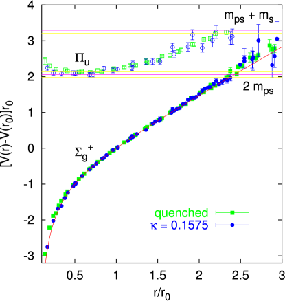
Figure 1: The heavy-quark potential $V(r)$ vs. $r$, computed with lattice QCD (line and points labeled $\Sigma_{g}^{+}$). From Ref. [18]. (The line and points labeled $\Pi_{u}$ denote an excitation of the interquark chromoelectric field.)

In addition to this appealing picture, lattice QCD has been used to verify the mass spectrum of hadrons quantitatively, within a few percent. Figure 2 shows three sets of results, each with specific compelling features.

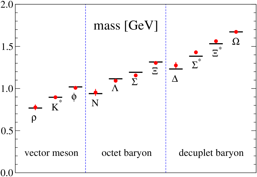
(a)
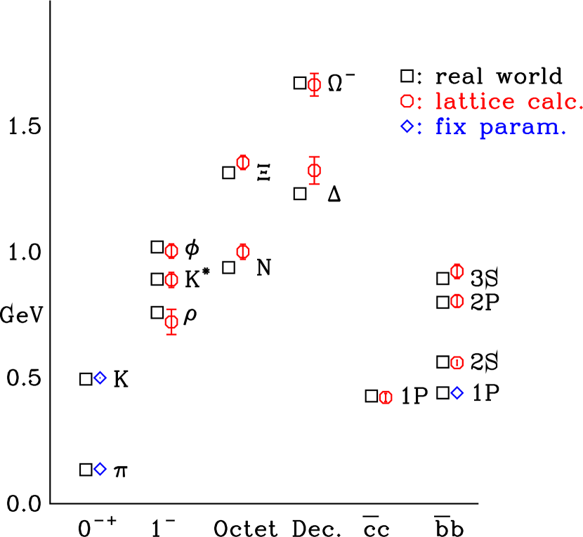
(b)        (c) 

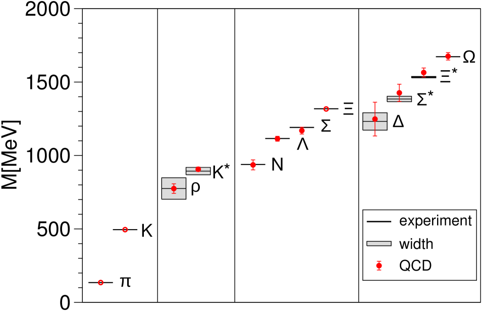
Figure 2: Hadron spectrum computed with lattice QCD by (a) the MILC Collaboration [19, 20], (b) the PACS-CS Collaboration [21], and (c) the BMW Collaboration [22].

Unless noted below, the error bars on the calculations encompass all systematic uncertainties. Figure 2a shows the broadest attack on the spectrum [19, 20], including $b\bar{b}$ and $c\bar{c}$ states taken from Refs. [23, 24]. The baryon masses are less well determined than meson masses, partly because of larger statistical errors, and partly because the lattice formulation of light quarks in Refs. [19, 20] is sub-optimal for baryons. Figure 2b shows the spectrum with light in-simulation quark masses nearly as small as $\frac{1}{2}(m_{\rm u}+m_{\rm d})$ [21]. Such small quark masses are at the frontier, and the plot omits the error bar associated with the continuum limit. Finally, Fig. 2c shows a complete calculation with good control of the baryons [22]. In particular, the nucleon mass, which provides almost all the mass in everyday objects [25], has now been verified within 3.5% to arise principally from chromodynamics: $m=E/c^{2}$.

4 Chiral Symmetry Breaking

A striking feature of the hadron spectrum is that the pion has a small mass, around 135–140 MeV, when most other hadrons have masses five or more times larger. For example, $m_{\rho}=770$ MeV, $m_{p}=938$ MeV. To understand the origin of the difference, Nambu [6] applied lessons from superconductivity, noting (four years before quarks) that the pion’s mass could be constrained to vanish by a spontaneously broken axial symmetry, with a small amount of explicit symmetry breaking allowing it to be nonzero.

QCD explains the origin of this symmetry. If the up and down quarks can be neglected, the Lagrangian acquires an $\mathrm{SU}_{\mathrm{L}}(2)\times\mathrm{SU}_{\mathrm{R}}(2)$ symmetry, which provides a candidate axial symmetry. The consequences of spontaneous symmetry breaking were studied further by Goldstone [26], leading to a formula [27],

$$m_{\pi}^{2}\langle\bar{\psi}\psi\rangle=0,$$ (7)

when applied to QCD with massless up and down quarks. The flavor-singlet expectation value $\langle\bar{\psi}\psi\rangle$ is called the chiral condensate. If either factor on the left-hand side of Eq. (7) is nonzero, the other must vanish.

Twenty-five years ago, when the Lake Louise Winter Institute began, most physicists were confident that QCD was a good theory of the strong interactions, based on, for example, its explanation of Bjorken scaling in deep-inelastic scattering. Because QCD was considered right, and because Nambu’s picture of the pion was considered right, it was believed that QCD must generate a chiral condensate. There was, however, no direct calculation of $\langle\bar{\psi}\psi\rangle$ starting from the QCD Lagrangian, Eq. (1). Now there is. Lattice QCD shows [28]

$$\langle\bar{\psi}\psi\rangle=\left[242\pm 4^{+19}_{-18}~{}\mathrm{MeV}\right]^{3}\quad\mbox{($\overline{\rm MS}$ scheme at 2~{}GeV)},$$ (8)

where the first uncertainty is statistical and the second a combination of systematics. The quark masses have been adjusted to Nambu’s idealization, $m_{\rm u}=m_{\rm d}\to 0$, $m_{\rm s}$ physical. Spontaneous symmetry breaking also appears in two-flavor QCD [29]. The chiral condensate has been established by direct computation to be very significantly nonzero. QCD breaks chiral symmetries spontaneously.

5 SM Parameters

The Standard Model has 19 free parameters, or 28 if nonzero neutrino masses and mixings are taken into account:

• Gauge couplings: $\bm{\alpha_{\rm s}}$, $\alpha_{\rm QED}$, $\alpha_{\rm W}=(M_{\rm W}/v)^{2}/\pi$;

• Lepton masses and mixing: $m_{\nu_{1}}$, $m_{\nu_{2}}$, $m_{\nu_{3}}$, $m_{\rm e}$, $m_{\mu}$, $m_{\tau}$; $\theta_{12}$, $\theta_{23}$, $\theta_{13}$, $\delta_{\rm PMNS}$, $\alpha_{21}$, $\alpha_{31}$;

• Quark masses and mixing: $\bm{m_{\rm u}}e^{i\bm{\bar{\theta}}}$, $\bm{m_{\rm d}}$, $\bm{m_{\rm s}}$, $\bm{m_{\rm c}}$, $\bm{m_{\rm b}}$, $m_{\rm t}$; $\bm{V_{\rm us}}$, $\bm{V_{\rm cb}}$, $\bm{V_{\rm ub}}$, $\bm{\delta_{\rm KM}}$;

• Standard electroweak symmetry breaking: $v=246$ GeV, $\lambda=(M_{H}/v)^{2}/2$.

For ten or eleven of these parameters (bold), lattice QCD is either essential or important for determining their values of the natural world. Lattice field theory (without QCD) is also useful for shedding light on the Higgs self-coupling $\lambda$ [31] and the top-quark Yukawa coupling $y_{\mathrm{t}}=\sqrt{2}m_{\rm t}/v$ [32], for which consistency of the field theory precludes arbitrary values.

5.1 QCD Parameters

Owing to confinement, there is no way to measure quark masses in a way comparable to, say, the electron mass. Instead, a Lagrangian definition as in Eq. (1), with suitable choice of renormalization scheme, must be determined from measurable properties of hadrons. For the light quarks, the simplest hadronic property is simply the pseudoscalar mesons masses, with the physical value obtained when the pion and kaon masses agree with experiment. Three sets of results are shown in Table 1.

Table 1: Quark masses from lattice QCD converted to the $\overline{\rm MS}$ scheme and run to the scale indicated (first, second, third, and fifth columns). Also listed are charmed and bottom masses determined from $e^{+}e^{-}$ production (fourth column).

	Ref. [20]		Ref. [33]		Ref. [34]		Ref. [35]		Ref. [36]
$\bar{m}_{\rm u}(2~{}\textrm{GeV})$ [MeV]	1.9$\,\pm\,$	0.2	2.01$\,\pm\,$	0.14	2.37$\,\pm\,$	0.26
$\bar{m}_{\rm d}(2~{}\textrm{GeV})$ [MeV]	4.6$\,\pm\,$	0.3	4.79$\,\pm\,$	0.16	4.52$\,\pm\,$	0.30
$\bar{m}_{\rm s}(2~{}\textrm{GeV})$ [MeV]	88$\,\pm\,$	5	92.4$\,\pm\,$	1.5	97.7$\,\pm\,$	6.0
$\bar{m}_{\rm c}({\bf 3}~{}\textrm{GeV})$ [MeV]							986$\,\pm\,$	13	986$\,\pm\,$	10
$\bar{m}_{\rm b}({\bf 10}~{}\textrm{GeV})$ [MeV]							3610$\,\pm\,$	16	3617$\,\pm\,$	25

The results in the second column [33] are derived from mass ratios underlying those in the first column [20], as discussed below. The results in the third column are completely independent, in particular employing different methods for sea quarks and different approaches to electromagnetic effects.

There are two noteworthy features of these results. First, the up and down masses are very small, about 4 and 9 times the tiny electron mass. Quark masses arise from interactions with the Higgs field, or its surrogate in other models of eletroweak symmetry. This sector is, thus, not the origin of much mass. Second, $m_{\rm u}$, though very small, is also very significantly far from zero. This is interesting, because were $m_{\rm u}=0$, then the additional symmetry of the Lagrangian would render $\bar{\theta}$ unphysical, obviating the strong CP problem.

The heavy charmed, bottom, and top quark masses are large enough that they can be determined with perturbative QCD from features of high-energy scattering cross sections and energy distributions. For example, using perturbation theory to $\mathrm{O}(\alpha_{\rm s}^{3})$ for the moments in $s$ of the cross section for $e^{+}e^{-}\to c\bar{c}$, as a function of center-of-mass energy-squared $s$, one finds the result in the fourth column, fourth row of Table 1. The $e^{+}e^{-}$ data can be replaced with moments of the charmonium correlation function, calculated with lattice QCD [37, 38]. Applying the same perturbative analysis yields the result in the fifth column, with astonishingly good agreement. The same methods can be applied to bottom quarks, also shown in Table 1.

Returning to the light-quark masses, the new result of Ref. [33] is a precise value of the (scheme independent) ratio $m_{\rm c}/m_{\rm s}=11.85\pm 0.16$. Combining this ratio with $\bar{m}_{c}$ [38]and the ratios $2m_{\rm s}/(m_{\rm d}+m_{\rm u})=27.3\pm 0.3$ and $m_{\rm u}/m_{\rm d}=0.42\pm 0.04$, both from Ref. [20], leads to the values in the second column of Table 1.

Lattice QCD also provides excellent ways to determine the gauge coupling $\alpha_{\rm s}=g^{2}/4\pi$. In lattice gauge theory, the bare coupling $g_{0}^{2}$ is an input. Alas, for most lattice gauge actions, perturbation theory in $g_{0}^{2}$ converges poorly [39], obstructing a perturbative conversion to the $\overline{\rm MS}$ or other such schemes. Two other strategies are adopted to circumvent this obstacle. One is to compute a short-distance lattice quantity—a Wilson loop, a Creutz ratio, or the potential at separations of order $a$—and reexpress perturbation theory for the Monte Carlo results in a way that eliminates $g_{0}^{2}$. The other is to compute a short-distance quantity with a continuum limit, and then apply continuum perturbation theory. The quarkonium correlator used for $m_{\rm c}$ and $m_{\rm b}$ is an example: it also yields $\alpha_{\rm s}(2m_{Q})$. Other examples include the Schrödinger functional [40] and the Adler function [41].

Results from several complementary lattice-QCD methods [38, 42, 43, 44] are collected in Table 2 and compared to an average of determinations from high-energy scattering and decays [45].

Table 2: Values of $\alpha_{\rm s}(M_{Z})$ from lattice QCD and an average of determinations from high-energy scattering and decays. A recent update to the values on the first two rows [42, 38] can be found in Ref. [36]. The central values and error bars from Refs. [43, 44] have been symmetrized to ease comparison.

$\alpha_{\rm s}(M_{Z})$		Observable	Sea formulation	Reference
0.1183$\,\pm\,$	0.0008	Wilson loops, Creutz ratios, etc.	2+1 asqtad staggered	HPQCD [42]
0.1174$\,\pm\,$	0.0012	charmonium correlator	2+1 asqtad staggered	HPQCD [38]
0.1197$\,\pm\,$	0.0013	Schrödinger functional	2+1 improved Wilson	PACS-CS [43]
0.1185$\,\pm\,$	0.0009	Adler function	2+1 overlap	JLQCD [44]
0.1186$\,\pm\,$	0.0011	scattering, $\tau$ decay, etc.	2+1(+1+1) Dirac (!)	Bethke [45]

One sees excellent consistency among results with different discretizations of the determinant for sea quarks. An important source of uncertainty is the truncation of perturbation theory, including strategies for matching to the $\overline{\rm MS}$ scheme, and running to scale $M_{Z}$. In the example of the lattice-scale loops, an independent analysis of the data from Ref. [42] has been carried out, yielding $\alpha_{\rm s}(M_{Z})=0.1192\pm 0.011$ [46], to be compared with the first line of Table 2.

As mentioned above, QCD is a union of the quark model of hadrons and the parton model of high-energy scattering. The agreement of the lattice-QCD results for $\alpha_{\rm s}$, as well as for $m_{\rm c}$ and $m_{\rm b}$, shows that hadrons and partons share the same QCD parameters, demonstrating QCD’s breadth: the QCD of hadrons is the QCD of partons.

5.2 Flavor Physics

Like the quark masses, the quark mixing, or Cabibbo-Kobayashi-Maskawa (CKM), matrix [47, 48] arises from the electroweak interactions. In the Standard Model, the masses are proportional to the eigenvalues of the Yukawa-coupling matrices between the quarks and the Higgs doublet. The CKM matrix is the observable part of the transformations from the fields interacting with the weak gauge bosons to their mass eigenstates. Symmetries of the gauge interactions make many components of these transformations unobervable. For three generations, three mixing angles and one CP-violating phase remain to account for all the flavor- and CP-violation in nature.

Lattice QCD calculations have played a key role in many aspects of flavor physics. A recent, comprehensive overview can be found in Ref. [49], so here we shall simply note some examples in which tension between the experiments and the Standard Model have appeared. These are tantalizing, because Standard CP violation seems insufficient to explain the baryon asymmetry of the universe. Tension appears in the global fit to the four CKM parameters [50] and also in several specific flavor-changing processes.

As anticipated, lattice-QCD calculations of neutral kaon mixing [51, 52] have improved such that the “standard” Standard-Model analysis had to re-incorporate certain effects of a few percent. (See Refs. [53, 54] for details.) With the re-improved formula, the tension in the global fit strengthens [54, 55].

Recent measurements of some purely leptonic decays $B^{+}\to\tau^{+}\nu$, $D_{s}\to\mu^{+}\nu$, and $D_{s}\to\tau^{+}\nu$ are somewhat in excess of the Standard-Model prediction for the branching ratio. A crucial ingredient are the decay constants $f_{B}$ and $f_{D_{s}}$ from lattice QCD [15, 56, 57, 58]. The nearly $2\sigma$ excess of $B^{+}\to\tau^{+}\nu$ is usually interpreted as a possible signal of charged Higgs bosons [59, 60], but then the non-Standard amplitude has to be around $-110$% of the Standard amplitude. The excesses of $D_{s}\to l^{+}\nu$ could be due to leptoquarks [61], with an few-percent amplitude constructively interfering. Note that the tension in this mode, which was once nearly $4\sigma$, is now below $2\sigma$, as improved calculations and, especially, new measurements have come out [62].

6 Thermodynamics

Like any physical system, QCD has thermodynamic properties. During the early universe, the temperature was much hotter than it is now. In neutron stars, the baryon density is much higher than in normal nuclear matter. A sketch of the phase diagram is shown in Fig. 3a, based on lattice-QCD studies and models [63].

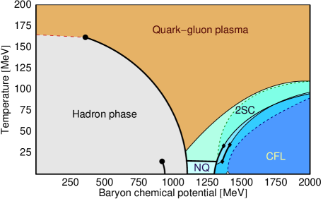
(a) (b)

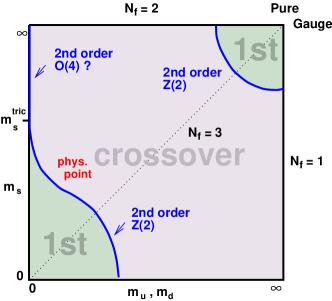
Figure 3: QCD phase diagrams, (a) in the $\mu$-$T$ plane (image from Ref. [63]); (b) at $\mu=0$, $T=T_{c}$, showing the order of the transition in the $m_{\rm s}$-$\frac{1}{2}(m_{\rm u}+m_{\rm d})$ plane (image from Ref. [64]).

A surprising result is that the transition between the hadronic phase and the “quark-gluon plasma” is a smooth crossover, rather than a first- or second-order phase transition [65, 66]. This means that as the early universe cools, the hot matter becomes more and more like a gas of distinct hadrons. With a genuine phase transition, bubbles of the hadronic phase would form. At nonzero baryon density (chemical potential $\mu$), it is thought that the transition becomes first order, but the matter is not yet settled [64]. For further discussion, see Refs [67, 68].

It may be worth clarifying what the quark-gluon plasma is. QCD thermodynamics is, as one would expect, based on the canonical ensemble, with thermal averages

$$\langle\bullet\rangle=\frac{\Tr\left[\bullet\,e^{-\hat{H}/T}\right]}{\Tr e^{-\hat{H}/T}},$$ (9)

where $T$ is the temperature. In quantum field theory formulated as in Eq. (2), the time extent $N_{4}$ specifies a temperature $T=(N_{4}a)^{-1}$. The trace $\Tr$ is over the Hilbert space of the QCD Hamiltonian $\hat{H}$. The eigenstates—aka hadrons—do not change with $T$, but as $T$ increases the propagation of a single source of color can change. First, thermal fluctuations encompass states with many overlapping hadrons, so color can propagate from one hadron to the next, as if deconfined. Second, the thermal average applies nearly equal weights to states of both parities, so chiral symmetry is restored—the thermal average of $\bar{\psi}\psi$ vanishes even if the vacuum expectation value does not. With a smooth crossover, these changes need not emerge at the same $T$, but, in practice, it seems they do [65, 66]. The picture of thermal averages over hadronic eigenstates and the crossover nature of the transition may help us understand why hadron gas models of the transition are so successful.

The nature of the QCD phase transition is influenced by the physical values of the light (up, down, and strange) quark masses, as sketched in Fig. 3b. For vanishing quark masses, the transition would be first order. The ratio $2m_{\rm s}/(m_{\rm u}+m_{\rm d})$ is well constrained by chiral symmetry (and substantiated by explicit calculation, as in Table 1). But the masses are just large enough to push the QCD system into the region of crossover. If the light quark masses—crucially $m_{\rm s}$—were around half their physical size, the universe would cool through a first-order transition. What kind of fluke is this?

7 Summary and Challenges

During the twenty-five years of the Lake Louise Winter Institute, lattice gauge theory has developed several ideas about QCD, nurturing them from “QCD should work this way” to “QCD does work this way.” Quantitative precision on $\alpha_{\rm s}$ and heavy-quark masses reassures us that the QCD of hadrons is the QCD of partons. Accurate calculations of the hadron masses and the chiral condensate show how QCD generates mass and that QCD breaks chiral symmetry. The dependence of hadron masses on quark masses leads to the conclusion that the masses generated via interaction with the Higgs field is very small. Your mass is $E/c^{2}$ from QCD. Furthermore, the up quark’s mass, though small, clearly does not vanish. The nonzero up, down, and strange masses make a qualitative difference to the early universe, because at physical quark mass (and low density) the QCD phase transition is actually a smooth crossover.

On the quantitative front, QCD faces many challenges. Hints of non-Standard processes in flavor physics require ever more precise calculations. It is fairly certain that the Standard amount of CP violation is insufficient to explain the baryon asymmetry, so it is plausible that one of these hints will settle into real evidence. The advent of the LHC calls for other calculations that still lie beyond today’s precision frontier of lattice QCD. For example, reliable moments of the gluon density inside the proton could help reduce uncertainties in LHC cross sections. If the LHC uncovers evidence for a dynamical mechanism breaking electroweak symmetry (similar in some, but not all, ways to QCD), lattice gauge theory will be necessary for non-QCD models (and, eventually, a new theory) [69, 70].

Nuclear physics is an arena where the need for computational lattice gauge theory is exploding [71]. In many cases, the same basic methods [Eqs. (3)–(5)] apply, but in others the technology has to be extended or invented [72]. Nuclear lattice QCD overlaps with astrophysics: better methods for nonzero baryon chemical potential would permit studies of the phases inside neutron stars, not to mention even denser phases shown in Fig. 3 [73]; meanwhile, calculations of hyperon-nucleon interactions shed light on strangeness in neutron stars [74].

References

- [1] Politzer H D 1973 Phys. Rev. Lett. 30 1346–1349
- [2] Gross D J and Wilczek F 1973 Phys. Rev. Lett. 30 1343–1346
- [3] Poggio E C, Quinn H R and Weinberg S 1976 Phys. Rev. D13 1958–1968
- [4] Wilson K G 1974 Phys. Rev. D10 2445–2459
- [5] Kim J E and Carosi G 2010 Rev. Mod. Phys. 82 557–601 (Preprint 0807.3125)
- [6] Nambu Y 1960 Phys. Rev. Lett. 4 380–382
- [7] Shifman M A and Voloshin M B 1987 Sov. J. Nucl. Phys. 45 292
- [8] Isgur N and Wise M B 1989 Phys. Lett. B232 113–117
- [9] Wilson K G 2005 Nucl. Phys. Proc. Suppl. 140 3–19 (Preprint hep-lat/0412043)
- [10] Sharpe S R and Shoresh N 2000 Phys. Rev. D62 094503 (Preprint hep-lat/0006017)
- [11] Bijnens J 2007 PoS LAT2007 004 (Preprint 0708.1377)
- [12] Davies C T H et al. (HPQCD, MILC, and Fermilab Lattice) 2004 Phys. Rev. Lett. 92 022001 (Preprint hep-lat/0304004)
- [13] Aubin C et al. (Fermilab Lattice and MILC) 2005 Phys. Rev. Lett. 94 011601 (Preprint hep-ph/0408306)
- [14] Allison I F et al. (HPQCD and Fermilab Lattice) 2005 Phys. Rev. Lett. 94 172001 (Preprint hep-lat/0411027)
- [15] Aubin C et al. (Fermilab Lattice and MILC) 2005 Phys. Rev. Lett. 95 122002 (Preprint hep-lat/0506030)
- [16] Kronfeld A S (Fermilab Lattice) 2006 J. Phys. Conf. Ser. 46 147–151 (Preprint hep-lat/0607011)
- [17] Juge K J, Kuti J and Morningstar C 2003 Phys. Rev. Lett. 90 161601 (Preprint hep-lat/0207004)
- [18] Bali G S 2001 Phys. Rept. 343 1–136 (Preprint hep-ph/0001312)
- [19] Aubin C et al. (MILC) 2004 Phys. Rev. D70 094505 (Preprint hep-lat/0402030)
- [20] Bazavov A et al. 2010 Rev. Mod. Phys. 82 1349–1417 (Preprint 0903.3598)
- [21] Aoki S et al. (PACS-CS) 2009 Phys. Rev. D79 034503 (Preprint 0807.1661)
- [22] Dürr S et al. (BMW) 2008 Science 322 1224–1227 (Preprint 0906.3599)
- [23] Gray A et al. (HPQCD) 2005 Phys. Rev. D72 094507 (Preprint hep-lat/0507013)
- [24] Burch T et al. (Fermilab Lattice and MILC) 2010 Phys. Rev. D81 034508 (Preprint 0912.2701)
- [25] Kronfeld A S 2008 Science 322 1198–1199 (Preprint FERMILAB-FN-0828-T)
- [26] Goldstone J 1961 Nuovo Cim. 19 154–164
- [27] Goldstone J, Salam A and Weinberg S 1962 Phys. Rev. 127 965–970
- [28] Fukaya H et al. (JLQCD) 2010 Phys. Rev. Lett. 104 122002 (Preprint 0911.5555)
- [29] DeGrand T, Liu Z and Schaefer S 2006 Phys. Rev. D74 094504 (Preprint hep-lat/0608019)
- [30] Petcov S T 2004 New J. Phys. 6 109
- [31] Gerhold P and Jansen K 2010 JHEP 1004 094 (Preprint 1002.4336)
- [32] Gerhold P and Jansen K 2009 JHEP 0907 025 (Preprint 0902.4135)
- [33] Davies C T H et al. (HPQCD) 2010 Phys. Rev. Lett. 104 132003 (Preprint 0910.3102)
- [34] Blum T et al. 2010 (Preprint 1006.1311)
- [35] Chetyrkin K G et al. 2009 Phys. Rev. D80 074010 (Preprint 0907.2110)
- [36] McNeile C, Davies C T H, Follana E, Hornbostel K and Lepage G P (HPQCD) 2010 (Preprint 1004.4285)
- [37] Bochkarev A and De Forcrand P 1996 Nucl. Phys. B477 489–520 (Preprint hep-lat/9505025)
- [38] Allison I et al. (HPQCD) 2008 Phys. Rev. D78 054513 (Preprint 0805.2999)
- [39] Lepage G P and Mackenzie P B 1993 Phys. Rev. D48 2250–2264 (Preprint hep-lat/9209022)
- [40] Lüscher M, Narayanan R, Weisz P and Wolff U 1992 Nucl. Phys. B384 168–228 (Preprint hep-lat/9207009)
- [41] Chetyrkin K G, Kühn J H and Steinhauser M 1996 Nucl. Phys. B482 213–240 (Preprint hep-ph/9606230)
- [42] Davies C T H et al. (HPQCD) 2008 Phys. Rev. D78 114507 (Preprint 0807.1687)
- [43] Aoki S et al. (PACS-CS) 2009 JHEP 10 053 (Preprint 0906.3906)
- [44] Shintani E et al. (JLQCD) 2010 (Preprint 1002.0371)
- [45] Bethke S 2009 Eur. Phys. J. C64 689–703 (Preprint 0908.1135)
- [46] Maltman K, Leinweber D, Moran P and Sternbeck A 2008 Phys. Rev. D78 114504 (Preprint 0807.2020)
- [47] Cabibbo N 1963 Phys. Rev. Lett. 10 531–533
- [48] Kobayashi M and Maskawa T 1973 Prog. Theor. Phys. 49 652–657
- [49] Laiho J, Lunghi E and Van de Water R S 2010 Phys. Rev. D81 034503 (Preprint 0910.2928)
- [50] Lunghi E and Soni A 2008 Phys. Lett. B666 162–165 (Preprint 0803.4340)
- [51] Antonio D J et al. (RBC and UKQCD) 2008 Phys. Rev. Lett. 100 032001 (Preprint hep-ph/0702042)
- [52] Aubin C, Laiho J and Van de Water R S 2010 Phys. Rev. D81 014507 (Preprint 0905.3947)
- [53] Anikeev K et al. 2001 Physics at the Tevatron: Run II and Beyond (Batavia: Fermilab) (Preprint hep-ph/0201071)
- [54] Buras A J and Guadagnoli D 2008 Phys. Rev. D78 033005 (Preprint 0805.3887)
- [55] Lunghi E and Soni A 2010 Phys. Rev. Lett. 104 251802 (Preprint 0912.0002)
- [56] Follana E, Davies C T H, Lepage G P and Shigemitsu J (HPQCD) 2008 Phys. Rev. Lett. 100 062002 (Preprint 0706.1726)
- [57] Gray A et al. (HPQCD) 2005 Phys. Rev. Lett. 95 212001 (Preprint hep-lat/0507015)
- [58] Bernard C et al. 2008 PoS LATTICE2008 278 (Preprint 0904.1895)
- [59] Akeroyd A G and Chen C H 2007 Phys. Rev. D75 075004 (Preprint hep-ph/0701078)
- [60] Deschamps O et al. 2009 (Preprint 0907.5135)
- [61] Dobrescu B A and Kronfeld A S 2008 Phys. Rev. Lett. 100 241802 (Preprint 0803.0512)
- [62] Kronfeld A S 2009 XXIX Physics in Collision ed Kawagoe K et al. (Tokyo: Universal Academy Press) (Preprint 0912.0543)
- [63] Rüster S B, Werth V, Buballa M, Shovkovy I A and Rischke D H 2005 Phys. Rev. D72 034004 (Preprint hep-ph/0503184)
- [64] de Forcrand P and Philipsen O 2008 JHEP 11 012 (Preprint 0808.1096)
- [65] Aoki Y, Endrodi G, Fodor Z, Katz S D and Szabo K K 2006 Nature 443 675–678 (Preprint hep-lat/0611014)
- [66] Bazavov A et al. 2009 Phys. Rev. D80 014504 (Preprint 0903.4379)
- [67] DeTar C and Heller U M 2009 Eur. Phys. J. A41 405–437 (Preprint 0905.2949)
- [68] Fodor Z and Katz S D 2010 Landolt-Börnstein 1/23a in press (Preprint 0908.3341)
- [69] Fleming G T 2008 PoS LATTICE2008 021 (Preprint 0812.2035)
- [70] Pallante E 2009 PoS LAT2009 015 (Preprint 0912.5188)
- [71] Beane S R, Orginos K and Savage M J 2008 Int. J. Mod. Phys. E17 1157–1218 (Preprint 0805.4629)
- [72] Bulava J M et al. 2009 Phys. Rev. D79 034505 (Preprint 0901.0027)
- [73] Alford M G, Schmitt A, Rajagopal K and Schäfer T 2008 Rev. Mod. Phys. 80 1455–1515 (Preprint 0709.4635)
- [74] Beane S R et al. (NPLQCD) 2007 Nucl. Phys. A794 62–72 (Preprint hep-lat/0612026)