Spreading speeds and traveling waves for a model of epidermal wound healing

Abstract

In this paper, we shall establish the spreading speed and existence of traveling waves for a non-cooperative system arising from epidermal wound healing and characterize the spreading speed as the slowest speed of a family of non-constant traveling wave solutions. Our results on the spreading speed and traveling waves can also be applied to a large class of non-cooperative reaction-diffusion systems.

1 Introduction

In this paper, we study the spreading speeds and traveling wave solutions of a non-cooperative reaction-diffusion systems arising from wound healing. Wound healing is complex and remains only partially understood, despite extensive research. Several reaction-diffusion models have been developed in Sherratt and Murray [23, 24], Dale, Maini, Sherratt [6] and others to understand the biological process of epidermal wound healing through mathematical analysis and numerical simulations. We refer to Murray [19] for more detailed discussions and further references. The models consist of two conservation equations, one for the epithelial cell density per unit area ($u_{1}(x,t)$) and one for the concentration of the mitosis-regulating chemical ($u_{2}(x,t)$). There are two types of the chemicals, one in which the chemical activates mitosis and the other in which it inhibits it. The following simplified model was proposed in [23, 19] for the activator

$$\begin{split}\frac{\partial u_{1}}{\partial t}&=d_{1}\Delta u_{1}+s(u_{2})u_{1}(2-u_{1})-u_{1}\\ \frac{\partial u_{2}}{\partial t}&=d_{2}\Delta u_{2}+b(h(u_{1})-u_{2})\\ \end{split}$$ (1.1)

where $b>0,\kappa\in(0,\frac{1}{2})$, $s(u_{2})=\kappa u_{2}+1-\kappa$ is the linearized function which reflects the chemical control of motosis. The chemical production by the function $h(u_{1})=\frac{u_{1}(1+\zeta^{2})}{u_{1}^{2}+\zeta^{2}},\zeta\in(0,1)$ reflects an appropriate cellular response to injury. The qualitative form of the solution of (1.1) in the linear phase is of a wave moving with constant shape and speed. Such a solution is amenable to analysis if we consider a cone dimensional geometry rather than the two dimensional radially symmetric geometry. Mathematically, we look for a traveling wave solution of the form $u_{1}(x,t)=u_{1}(\xi),u_{2}(x,t)=u_{2}(\xi),\xi=x+ct$ where $c$ is the wave speed, positive since here we consider waves moving to the left. In Section 4, we shall establish the existence of traveling waves as well as the results on the speed of propagation to (1.1). In addition, we characterize the minimum speed as the slowest speed of a family of non-constant traveling wave solutions of (1.1).

Traveling wave solutions and spreading speeds for reaction-diffusion equations have been studied by a number of researchers. Fisher [10] studied the nonlinear parabolic equation

$$w_{t}=w_{xx}+w(1-w).$$ (1.2)

for the spatial spread of an advantageous gene in a population and conjectured $c^{*}$ is the asymptotic speed of propagation of the advantageous gene. His results show that (1.2) has a traveling wave solution of the form $w(x+ct)$ if only if $|c|\geq c^{*}=2.$ Kolmogorov, Petrowski, and Piscounov [14] proved the similar results with more general model. Those pioneering work along with the paper by Aronson and Weinberger [1, 2] confirmed the conjecture of Fisher and established the speeding spreads for nonlinear parabolic equations. Lui [18] established the theory of spreading speeds for cooperative recursion systems. In a series of papers, Weinberger, Lewis and Li [15, 16, 31, 32] studied spreading speeds and traveling waves for more general cooperative recursion systems, and in particular, for quite general cooperative reaction-diffusion systems by analyzing of traveling waves and the convergence of initial data to wave solutions. However, mathematical challenges remain because many reaction-diffusion systems are not necessarily cooperative due to various biological or physical constrains. Thieme [26] showed that asymptotic spreading speed of integral equations with nonmonotone growth functions can still be obtained by constructing monotone functions. For a related nonmonotone integro-difference equation, Hsu and Zhao [12], Li, Lewis and Weinberger [17] extended the theory of spreading speed and established the existence of travel wave solutions. The author and Castillo-Chavez [29] prove that a class of nonmonotone integro-difference systems have spreading speeds and traveling wave solutions. Such an extension is largely based on the construction of two monotone operators with appropriate properties and fixed point theorems in Banach spaces. A similar method was also used in Ma [22] and the author [28] to prove the existence of traveling wave solutions of nonmonotone reaction-diffusion equations. Weinberger, Kawasaki and Shigesada [35] discuss the minimum spreading speeds for a partially-cooperative system describing the interaction between ungulates and grass. It is cooperative for small population densities but not for large ones. By employing comparison methods [35] established the spreading speeds of propagation. In a recent paper [30], we study traveling waves and spreading speeds of propagation for a class of non-cooperative reaction-diffusion systems and a slightly different model describing the interaction between ungulates and grass.

In this paper, we shall study the spreading speeds and existence of traveling waves for the non-cooperative system arising from epidermal wound healing (1.1). The minimum speed $c^{*}$ can be characterized as the slowest speed of a family of non-constant traveling wave solutions. In other words, we shall show that for $c\geq c^{*}$ (1.1) always has a nonconstant traveling solutions of the form $(u_{1}(x+ct),u_{2}(x+ct))$ with $(u_{1}(-\infty),u_{2}(-\infty))=0$ but bounded away from zero at $+\infty$, and there is no such traveling solution when $0\leq c<c^{*}.$ Our main results for the epidermal wound healing model are summarized in Theorem 4.1. The results for general non-cooperative systems (2.3) are included in Theorem 2.2. In Section 4 we shall verify the assumptions of Theorem 2.2 for (1.1) and apply the general results to (1.1).

In order to better understanding of the spreading speeds and traveling solutions for the epidermal wound healing model. The general results in this paper have some significant improvements of those results over [30]. For example, in this paper we make use of the comparison principle from Fife [9]. Another form of the comparison principle from [35] was used in [30]. As a result, the assumptions (H1-H2) and the proofs in Section 5 are somewhat different from [30]. By a suitable modification of the functions, the conditions in this paper seem easier to verify. In addition, Theorem 3.1 is more general than that in [30], for example, $d_{1}\geq d_{2}$ is imposed in [30]. To take $d_{1}<d_{2}$ into consideration, some assumptions and proofs are substantially modified. In particular, for this epidermal wound healing model, we show that the condition for Theorem 3.1(ii) can be satisfied if $u_{1}(x)\not\equiv 0$. Finally, verifications of lower and upper solutions for the equivalent integral equations are significantly simplified via a result in Ma [21]. In [28] and [30], a more direct but lengthy verification of the lower and upper solutions are given for scalar and n-dimensional systems respectively. We also omit some standard proofs such as continuity and compactness for the operator which can be found in previous papers.

2 Preliminaries

We begin with some notation. We shall use $R,k,k^{\pm},f,f^{\pm},r,u,v$ to denote vectors in $\mathbb{R}^{N}$ or $N$-vector valued functions , and $x,y,\xi$ the single variable in $\mathbb{R}$. Let $u=(u_{i}),v=(v_{i})\in\mathbb{R}^{N}$, we write $u\geq v$ if $u_{i}\geq v_{i}$ for all $i$; and $u\gg v$ if $u_{i}>v_{i}$ for all $i$. We further define for any $r=(r^{i})>>0,r\in\mathbb{R}^{N}$ the ${R}^{N}$-interval

$$[0,r]=\{u:0\leq u\leq r,u\in\mathbb{R}^{N}\}\subseteq\mathbb{R}^{N}$$

and

$$\mathcal{C}_{r}=\{u=(u_{i}):u_{i}\in C(\mathbb{R},\mathbb{R}),0\leq u_{i}(x)\leq r_{i},x\in\mathbb{R},\;i=1,...,N\},$$

where $C(\mathbb{R},\mathbb{R})$ is the set of all continuous functions from $\mathbb{R}$ to $\mathbb{R}$.

Consider the system of reaction-diffusion equations

$$u_{t}=Du_{xx}+f(u),x\in\mathbb{R},\;t\geq 0.$$ (2.3)

with

$$u(x,0)=u_{0}(x),\;\;x\in\mathbb{R},$$ (2.4)

where $u=(u_{i})$, $D=\text{diag}(d_{1},d_{2},...,d_{N}),d_{i}>0,i=1,...,N$

$$f(u)=(f_{1}(u),f_{2}(u),...,f_{N}(u)),$$

$u_{0}(x)$ is a bounded uniformly continuous function on $\mathbb{R}.$ In this paper, by a solution we mean a twice continuously differentiable function $u(x,t)$ in $\mathbb{R}\times(0,\infty)$ and continuous in $\mathbb{R}\times[0,\infty)$, and satisfying appropriate equation in $\mathbb{R}\times(0,\infty)$ and an initial condition.

In order to deal with non-cooperative system, we shall assume that there are additional two monotone operators $f^{\pm}$, one lies above and another below $f$ with the corresponding equations

$$u_{t}=Du_{xx}+f^{+}(u),x\in\mathbb{R},\;t\geq 0.$$ (2.5)

$$u_{t}=Du_{xx}+f^{-}(u),x\in\mathbb{R},\;t\geq 0.$$ (2.6)

Such an assumption will enable us to make use of the corresponding results for cooperative systems in [18, 31] to establish spreading speeds for (2.3).

1. • Let $f,f^{\pm}:\mathbb{R}^{N}\to\mathbb{R}^{N}$ be Lipschitz continuous, twice piecewise continuous differentiable function such that

     $$f^{-}(u)\leq f(u)\leq f^{+}(u),u\in\mathbb{R}^{N}.$$

   • Let $0<<k^{-}=(k^{-}_{i})\leq k=(k_{i})\leq k^{+}$ and $f(0)=f(k)=0$ and assume that there is no other positive equilibrium of $f$ between $0$ and $k$ (that is, there is no constant $v\neq k$ such that $f(v)=0,0<<v\leq k$). $f^{\pm}(0)=f^{\pm}(k^{\pm})=0$. There is no other positive equilibrium of $f^{\pm}$ between $0$ and $k^{\pm}$.

   • (2.5) and (2.6) are cooperative (i.e. $\partial_{i}f^{\pm}_{j}(u)\geq 0$ for $u\in[0,k^{+}],i\neq j$). $f^{\pm}(u),f(u)$ have the same Jacobian matrix $f^{\prime}(0)$ at $u=0$.

A traveling wave solution $u$ of (2.3) is a solution of the form $u=u(x+ct),u\in C(\mathbb{R},\mathbb{R}^{N})$ . Substituting $u(x,t)=u(x+ct)$ into (2.3) and letting $\xi=x+ct$, we obtain the wave equation

$$Du^{\prime\prime}(\xi)-cu^{\prime}(\xi)+f(u(\xi))=0,\;\;\xi\in\mathbb{R}.$$ (2.7)

Now if we look for a solution of the form $(u_{i})=\big{(}e^{\lambda\xi}\eta^{i}_{\lambda}\big{)},\lambda>0,\eta_{\lambda}=(\eta^{i}_{\lambda})>>0$ for the linearization of (2.7) at the origin, we arrive at the following system equation

$$\text{diag}(d_{i}\lambda^{2}-c\lambda)\eta_{\lambda}+f^{\prime}(0)\eta_{\lambda}=0$$

which can be rewritten as the following eigenvalue problem

$$\frac{1}{\lambda}A_{\lambda}\mathbf{\eta_{\lambda}}=c\mathbf{\eta_{\lambda}},$$ (2.8)

where

$$A_{\lambda}=(a^{i,j}_{\lambda})=\text{diag}(d_{i}\lambda^{2})+f^{\prime}(0)$$

The matrix $f^{\prime}(0)$ has nonnegative off diagonal elements. In fact, there is a constant $\alpha$ such that $f^{\prime}(0)+\alpha I$ has nonnegative entries, where $I$ is the identity matrix.

By reordering the coordinates, we can assume that $f^{\prime}(0)$ is in block lower triangular form, in which all the diagonal blocks are irreducible or $1$ by $1$ zero matrix. A matrix is irreducible if it is not similar to a lower triangular block matrix with two blocks via a permutation. Let $\rho(A)$ be the spectral radius of $A$. For a matrix $A$ with nonnegative off diagonal elements, from the Perron-Frobenius theorem, we shall call the eigenvalue

$$\Psi(A)=\rho(A+\alpha I)-\alpha$$

of $A$, which has the same eigenvector, the principal eigenvalue of $A$ (see e.g. [11, 31]). Here $A+\alpha I$ is nonnegative, and $\rho(A+\alpha I)$ is the spectral radius of $A+\alpha I.$

We make assumptions on $A_{\lambda}$ and also requires $f$ grows less than its linearization along the particular function $\nu_{\lambda}e^{-\lambda x}$ [31]. Such a condition can be satisfied for many biological systems.

1. • Assume that $A_{\lambda}$ is in block lower triangular form and the first diagonal block has the positive principal eigenvalue $\Psi(A_{\lambda})$, and $\Psi(A_{\lambda})$ is strictly larger than the principal eigenvalues of all other diagonal blocks for some interval $[0,\Lambda^{*}]$ of $\lambda$. Assume that for $\lambda\in[0,\Lambda^{*}]$ (we also assume that $\Lambda_{c^{*}}\leq\Lambda^{*}\leq\infty$, see Lemma 2.1 for $\Lambda_{c^{*}}$), there is a positive eigenvector $\nu_{\lambda}=(\nu^{i}_{\lambda})>>0$ of $A_{\lambda}$ corresponding to $\Psi(A_{\lambda})$.

   • Assume that for each $\lambda\in[0,\Lambda^{*}]$, $\theta>0$

     $$f^{\pm}(\theta\nu^{i}_{\lambda})\leq f^{\prime}(0)\theta\nu^{i}_{\lambda}.$$

Let

$$\Phi(\lambda)=\frac{1}{\lambda}\Psi(A_{\lambda})>0.$$

According to Lemma 2.1, we can expect the graph of $\Phi$ as in Fig. 1. For the example in Section 4, $\Phi$ is a strictly convex function of $\lambda$ and, clearly satisfies Lemma 2.1.

Now we state Lemma 2.1, which is a analogous result in Weinberger [34] and Lui [18]. However, due to the fact that $f^{\prime}(0)$ is only quasi-positive and the elements of $A_{\lambda}$ are not necessarily log convex, some of its proof here are different from Lui [18]. A similar result is included in [30]. A theorem on the convexity of the dominant eigenvalue of matrices due to Cohen [4] is used to show that $\Psi(A_{\lambda})$ is convex function of $\lambda$. Lemma 2.1 improves [31, Theorem 4.2] by eliminating the case (b) in [31, Theorem 4.2].

Lemma 2.1

Assume that $(H1)-(H2)$ hold. Then

1. $\Phi(\lambda)\to\infty$ as $\lambda\to 0;$

2. If $\Lambda^{*}=\infty$, $\Phi(\lambda)\to\infty$ as $\lambda\to\infty;$

3. $\Phi(\lambda)$ is decreasing as $\lambda=0^{+};$

4. $\Psi(A_{\lambda})$ is a convex function of $\lambda>0;$

5. $\Phi^{\prime}(\lambda)$ changes sign at most once on $(0,\infty)$

6. $\Phi(\lambda)$ has the minimum

   $$c^{*}=\inf_{\lambda>0}\Phi(\lambda)>0$$

   at a finite $\Lambda_{c^{*}}>0$.

7. For each $c>c^{*}$, there exist a positive $\Lambda_{c}<\Lambda_{c^{*}}$ and $\gamma\in(1,\min\{2,\frac{\Lambda_{c^{*}}}{\Lambda_{c}}\})$ such that

   $$\Phi(\Lambda_{c})=c,\;\;\Phi(\gamma\Lambda_{c})<c.$$

   That is

   $$\frac{1}{\Lambda_{c}}A_{\Lambda_{c}}\nu_{\Lambda_{c}}=\Phi(\Lambda_{c})\nu_{\Lambda_{c}}=c\nu_{\Lambda_{c}}$$

   and

   $$\frac{1}{\gamma\Lambda_{c}}A_{\gamma\Lambda_{c}}\nu_{\gamma\Lambda_{c}}=\Phi(\gamma\Lambda_{c})\nu_{\gamma\Lambda_{c}}<c\nu_{\gamma\Lambda_{c}}$$

   where $\nu_{\Lambda_{c}}>>0,\nu_{\gamma\Lambda_{c}}>>0$ are positive eigenvectors of $\frac{1}{\Lambda_{c}}A_{\Lambda_{c}},\frac{1}{\gamma\Lambda_{c}}A_{\gamma\Lambda_{c}}$ corresponding to eigenvalues $\Phi(\Lambda_{c})$ and $\Phi(\gamma\Lambda_{c})$ respectively.

[Proof.]The proof of the convexity of $\Psi(A_{\lambda})$ is similar to that in Crooks [5] for matrices with positive off-diagonal elements. It is easily seen that $\Psi(A_{\lambda})=\rho(A_{\lambda}+\alpha I)-\alpha$ is non-decreasing function of $\lambda>0$ ([11, Theorem 8.1.18]). Further, a theorem on the convexity of the dominant eigenvalue of matrices due to Cohen [4] states that for any positive diagonal matrices $D_{1},D_{2}$ and $t\in(0,1)$,

$$\Psi(tD_{1}+(1+t)D_{2}+f^{\prime}(0))\leq t\Psi(D_{1}+f^{\prime}(0))+(1-t)\Psi(D_{2}+f^{\prime}(0))$$

as before, here $\Psi(A)$ is the principle eigenvalue of $A$. Now if $\alpha_{1},\alpha_{2}\in\mathbb{R}$ and $t\in(0,1)$,

$$(t\alpha_{1}+(1-t)\alpha_{2})^{2}\leq t\alpha_{1}^{2}+(1-t)\alpha_{2}^{2}.$$

This implies that

$$\begin{split}\Psi(A_{t\lambda_{1}+(1-t)\lambda_{2}})&=\Psi((t\lambda_{1}+(1-t)\lambda_{2})^{2}D+f^{\prime}(0))\\ &\leq\Psi(t\lambda_{1}^{2}D+(1-t)\lambda_{2}^{2}D+f^{\prime}(0))\\ &\leq t\Psi(\lambda_{1}^{2}D+f^{\prime}(0))\\ &\quad+(1-t)\Psi(\lambda_{2}^{2}D+f^{\prime}(0))\\ &=t\Psi(A_{\lambda_{1}})+(1-t)\Psi(A_{\lambda_{2}})\\ \end{split}$$

Since $\Psi(A_{\lambda})$ is a simple root of the characteristic equation of an irreducible block, it can be shown that $\Psi(A_{\lambda})$ is twice continuously differentiable on $\mathbb{R}$. Thus

$$\Psi^{\prime\prime}(\lambda)\geq 0$$

and a calculation shows

$$[\lambda\Phi(\lambda)]^{\prime}=\Psi^{\prime}(\lambda)$$

$$\Phi^{\prime}(\lambda)=\frac{1}{\lambda}[\Psi^{\prime}(\lambda)-\Phi(\lambda)]$$

and

$$(\lambda^{2}\Phi^{\prime}(\lambda))^{\prime}=\lambda\Psi^{\prime\prime}(\lambda)\geq 0.$$

As for (2), we need to prove that $\lim_{\lambda\to\infty}\frac{\Psi(A_{\lambda})}{\lambda}=\infty$. In fact, there exists an $\epsilon>0$ such that all diagonal elements of $D-\epsilon I$ are strictly positive, then $\Psi\big{(}D-\epsilon I\big{)}>0$ and choose $\lambda$ large enough so that

$$\begin{split}\Psi(A_{\lambda})&=\Psi(D\lambda^{2}+f^{\prime}(0))\\ &=\Psi\big{(}(D-\epsilon I)\lambda^{2}+(\epsilon\lambda^{2}I+f^{\prime}(0))\big{)}\\ &\geq\Psi\big{(}(D-\epsilon I)\lambda^{2}\big{)}\\ &=\lambda^{2}\Psi\big{(}D-\epsilon I\big{)}\end{split}$$

Thus $\lim_{\lambda\to\infty}\frac{\Psi(A_{\lambda})}{\lambda}=\infty$. (6) is a consequence of (1)-(5). (7) is a direct consequence of (1)-(6). It is just the fact that $\nu_{\lambda}>>0$ is a eigenvector of $\frac{1}{\lambda}A_{\lambda}$ corresponding to eigenvalue $\Phi(A_{\lambda})$ for $\lambda=\Lambda_{c}$ and $\gamma\Lambda_{c}$. $\quad\Box$

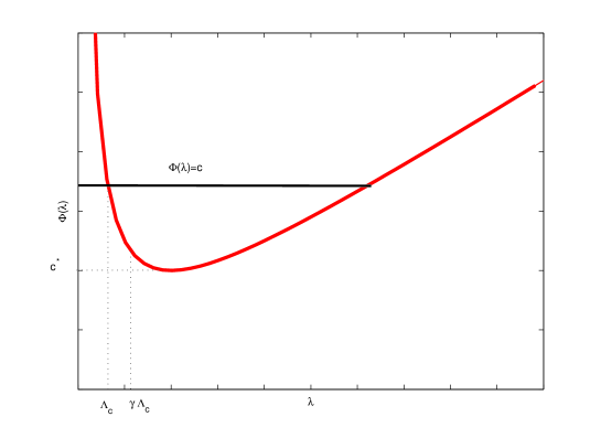
Figure 1: The red curve is $\Phi(\lambda)$. The minimum of $\Phi(\lambda)$ is $c^{*}$. For $c>c^{*}$, the left solution of $\Phi(\lambda)=c$ is $\Lambda_{c}$.

We now recall results on the spreading speeds in Weinberger, Lewis and Li [31] and Lui [18]. While Theorem 4.1 [31] holds for non cooperative reaction-diffusion systems, it does require that the reaction-diffusion system has a single speed. In general, such a condition is very difficult to verify. In the same section, for cooperative systems, Theorem 4.2 in [31] provides sufficient conditions to have a single speed. The following theorem combines the results of Theorems 4.1 and 4.2 in [31], which can be a consequence of Theorems 3.1 and 3.2 for discrete-time recursions in Lui [18].

Theorem 2.2

(Weinberger, Lewis and Li [31]) Assume $(H1)-(H2)$ hold and (2.3) is cooperative. Then the following statements are valid:

1. For any $u_{0}\in\mathcal{C}_{k}$ with compact support, let $u(x,t)$ be the solution of (2.3) with (2.4). Then

   $$\lim_{t\to\infty}\sup_{\lvert x\rvert\geq ct}u(x,t)=0,\text{ for }c>c^{*}$$

2. For any strictly positive vector $\omega\in\mathbb{R}^{N}$, there is a positive $R_{\omega}$ with the property that if $u_{0}\in\mathcal{C}_{k}$ and $u_{0}\geq\omega$ on an interval of length $2R_{\omega}$, then the solution $u(x,t)$ of (2.3) with (2.4) satisfies

   $$\liminf_{t\to\infty}\inf_{\lvert x\rvert\leq tc}u(x,t)=k,\text{ for }0<c<c^{*}$$

In another paper [16], for cooperative systems, Li, Weinberger and Lewis established that the slowest spreading speed $c^{*}$ can always be characterized as the slowest speed of a family of traveling waves. These results describe the properties of spreading speed $c^{*}$ for monotone systems. Based on these spreading results for cooperative systems, we will discuss analogous spreading speed results for non cooperative systems.

3 Results on general non-cooperative systems

In this section, we state a theorem for general partially cooperative reaction-diffusion systems (2.3) which establishes the existence of traveling waves and spreading speed for a large class of non-cooperative systems. As we discussed in Section 2, assumptions (H1-H2) and the proofs in Section 5 are different from those in [30] and the assumptions seem easier to verify. Although the existence of traveling wave solutions for cooperative systems are known (see,e.g. [16]), we shall prove the existence of traveling wave solutions for both cooperative and non cooperative systems as our proofs for non cooperative systems are based on those for cooperative systems. Further, in additions to the existence of traveling wave solutions, we shall be able to obtain asymptotic behavior of the traveling wave solutions in terms of eigenvalues and eigenvectors for both cooperative and non cooperative systems. The following theorem is our results for general non-cooperative reaction-diffusion systems.

Theorem 3.1

Assume $(H1)-(H2)$ hold. Then the following statements are valid:

1. For any $u_{0}\in\mathcal{C}_{k}$ with compact support, the solution $u(x,t)$ of (2.3) with (2.4) satisfies

   $$\lim_{t\to\infty}\sup_{\lvert x\rvert\geq tc}u(x,t)=0,\text{ for }c>c^{*}$$

2. For any vector $\omega\in\mathbb{R}^{N},\omega>>0$, there is a positive $R_{\omega}$ with the property that if $u_{0}\in\mathcal{C}_{k}$ and $u_{0}\geq\omega$ on an interval of length $2R_{\omega}$, then the solution $u(x,t)$ of (2.3) with (2.4) satisfies

   $$k^{-}\leq\liminf_{t\to\infty}\inf_{\lvert x\rvert\leq tc}u(x,t)\leq k^{+},\text{ for }0<c<c^{*}$$

3. For each $c>c^{*}$ (2.3) admits a traveling wave solution $u=u(x+ct)$ such that $0<<u(\xi)\leq k^{+},\xi\in\mathbb{R}$,

   $$k^{-}\leq\liminf_{\xi\to\infty}u(\xi)\leq\limsup_{\xi\to\infty}u(\xi)\leq k^{+}$$

   and

   $$\lim_{\xi\to-\infty}u(\xi)e^{-\Lambda_{c}\xi}=\nu_{\Lambda_{c}}.$$ (3.9)

   If, in addition, (2.3) is cooperative in $\mathcal{C}_{k}$, then $u$ is nondecreasing on $\mathbb{R}$.

4. For $c=c^{*}$ (2.3) admits a nonconstant traveling wave solution $u=u(x+ct)$ such that $0\leq u(\xi)\leq k,\xi\in\mathbb{R}$,

   $$k^{-}\leq\liminf_{\xi\to\infty}u(\xi)\leq\limsup_{\xi\to\infty}u(\xi)\leq k^{+}.$$

5. For $0<c<c^{*}$ (2.3) does not admit a traveling wave solution $u=u(x+ct)$ with $\liminf_{\xi\to\infty}u(\xi)>>0$ and $u(-\infty)=0.$

Remark 3.2

In many cases, $f^{\pm}$ can be taken as piecewise functions consisting of $f$ and appropriate constants as demonstrated in Section 4. In order to have a better estimate for the traveling wave solution $u$ for non cooperative systems, it is desirable to choose two function $f^{\pm}$ which are close enough. The smallest monotone function above $f$ and the largest monotone function below $f$ are natural choices of $f^{\pm}$ if they satisfy other requirements, See [26, 12, 17] for the discussion for scalar cases and [35] for a partially cooperative reaction-diffusion system. Our construct of $f^{-}$ in Section 4 is different from the previous papers.

Remark 3.3

When (2.3) is cooperative in $\mathcal{C}_{k}$, then $f^{\pm}=f.$

Remark 3.4

Assumptions (H1)(i-ii) imply that $\mathcal{C}_{k^{+}}$ is an invariant set of (2.3) in the sense that for any given $u_{0}\in\mathcal{C}_{k^{+}}$, the solution of (2.3) with the initial condition $u_{0}$ exists and remains in $\mathcal{C}_{k^{+}}$ for $t\in[0,\infty)$. In fact, for a given $u_{0}\in\mathcal{C}_{k^{+}}$, let $u(x,t)$ be the solution of (2.3) with the initial condition $u_{0}$. Theorem 5.1 implies that

$$0\leq u(x,t)\leq k^{+},x\in\mathbb{R},t>0.$$

Now according to Smoller [25, Theorem 14.4] (2.3) (and also (2.5), (2.6)) has a solution $u$ for $t\in[0,\infty)$ and $0\leq u\leq k^{+}$ if the initial value $u_{0}$ is uniformly continuous on $\mathbb{R}$.

We shall prove Theorem 3.1 (i)-(iii) in Section 5 and (iii)-(v) in Section 6.

4 Results on a model arising from epidermal wound healing

In Section 4, we shall apply the general results in Section 3 to the model (1.1) arising from epidermal wound healing. This model is not cooperative because of the fact that $h(u_{1})$ is not monotone. We shall establish the existence of traveling waves as well as the results on the speed of propagation to (1.1). In addition, we characterize the spreading speed as the slowest speed of a family of non-constant traveling wave solutions of (1.1). The spreading speed for (1.1) was discussed in [24, 19] based on numerical methods and singular perturbation techniques for several special cases, for example, $d_{1}=0$.

Recall that $h(u_{1})=\frac{u_{1}(1+\zeta^{2})}{u_{1}^{2}+\zeta^{2}}$. It is easy to (1.1) has two equilibria $(0,0)$ and $(1,1)$. In fact, the following equalities hold at its non-trivial equilibrium

$$\begin{split}h(u_{1})&=\frac{\frac{1}{2-u_{1}}+\kappa-1}{\kappa}\\ u_{2}&=h(u_{1}).\end{split}$$ (4.10)

Now it is clear that (4.10) has only one positive solution $(1,1).$ In fact, $\frac{\frac{1}{2-u_{1}}+\kappa-1}{\kappa}$ in (4.10) is increasing and convex on $(0,\infty)$ and the first equation of (4.10) has only one solution $u_{1}=1$.

We now need to check (H2). The linearization of (1.1) at the origin is

$$\begin{split}\frac{\partial u_{1}}{\partial t}&=d_{1}\Delta u_{1}+(1-2\kappa)u_{1}\\ \frac{\partial u_{2}}{\partial t}&=d_{2}\Delta u_{2}+b(h^{\prime}(0)u_{1}-u_{2})\end{split}$$ (4.11)

where $h^{\prime}(0)=\frac{1+\zeta^{2}}{\zeta^{2}}.$ The matrix $A_{\lambda}$ in (2.8) for (1.1) is

$$\begin{split}A_{\lambda}=(a^{i,j}_{\lambda})=\left(\begin{array}[]{ll}d_{1}\lambda^{2}+1-2\kappa&\;\;\;0\\ bh^{\prime}(0)&d_{2}\lambda^{2}-b\\ \end{array}\right)\end{split}$$ (4.12)

It is easy to see that

$$\begin{split}h(u_{1})<h^{\prime}(0)u_{1},\;\;u_{1}\in(0,\infty).\end{split}$$ (4.13)

In order to use Theorem 3.1, we shall define the two monotone systems. Note that $h(u_{1})$ achieves its maximum value $\frac{1+\zeta^{2}}{2\zeta}$ when $u_{1}=\zeta.$

$$h^{+}(u_{1})=\left\{\begin{array}[]{ll}h(u_{1}),&\;\;\;\;\;0\leq u_{1}\leq\zeta,\\[5.69046pt] h(\zeta),&\;\;\;\;\;u_{1}\geq\zeta.\end{array}\right.$$

and the corresponding cooperative system is

$$\begin{split}\frac{\partial u_{1}}{\partial t}&=d_{1}\Delta u_{1}+s(u_{2})u_{1}(2-u_{1})-u_{1}\\ \frac{\partial u_{2}}{\partial t}&=d_{2}\Delta u_{2}+b(h^{+}(u_{1})-u_{2})\\ \end{split}$$ (4.14)

In a similar manner, one can find (4.14) has two equilibrium $(0,0)$ and $(k_{1}^{+},k_{2}^{+})$ satisfying

$$\begin{split}h^{+}(k_{1}^{+})&=\frac{\frac{1}{2-k_{1}^{+}}+\kappa-1}{\kappa}\\ k_{2}^{+}&=h^{+}(k_{1}^{+}).\end{split}$$ (4.15)

Since $h^{+}=h$ for $u_{1}\leq\zeta$, then $k_{1}^{+}>\zeta$ (if $k_{1}^{+}\leq\zeta$ , then $k^{+}_{1}=1$ and $\zeta\geq 1$) and $h^{+}(k_{1}^{+})=\frac{1+\zeta^{2}}{2\zeta}$. Solving $k_{1}^{+}$ directly from (4.15) gives that $k_{1}^{+}=2-\frac{1}{1+(\frac{1+\zeta^{2}}{2\zeta}-1)\kappa}>1>\zeta$. It follows that $k^{+}_{2}=h^{+}(k_{1}^{+})=\frac{1+\zeta^{2}}{2\zeta}>1$.

Now there is a $h_{0}\in(0,\zeta]$ such that $h(h_{0})<\min\{1,h(k_{1}^{+})\}$ and define

$$h^{-}(u_{1})=\left\{\begin{array}[]{ll}h(u_{1}),&\;\;\;0\leq u_{1}\leq h_{0},\\[5.69046pt] h(h_{0}),&\;\;\;u_{1}>h_{0}.\end{array}\right.$$

It is clear that

$$0<h^{-}(u_{1})\leq h(u_{1})\leq h^{+}(u_{1})\leq h^{\prime}(0)u_{1},u_{1}\in(0,k^{+}_{1}]$$

and $h^{-}(u_{1})<1$ for $u_{1}\geq 0.$

Figure 2: The construction of $h^{+}$ and $h^{-}$. The red curve is $h$.

The corresponding cooperative system for $h^{-}$ is

$$\begin{split}\frac{\partial u_{1}}{\partial t}&=d_{1}\Delta u_{1}+s(u_{2})u_{1}(2-u_{1})-u_{1}\\ \frac{\partial u_{2}}{\partial t}&=d_{2}\Delta u_{2}+b(h^{-}(u_{1})-u_{2})\\ \end{split}$$ (4.16)

In a similar manner, one can find (4.16) has two equilibrium $(0,0)$ and $(k_{1}^{-},k_{2}^{-})$ satisfying

$$\begin{split}h^{-}(k_{1}^{-})&=\frac{\frac{1}{2-k_{1}^{-}}+\kappa-1}{\kappa}\\ k_{2}^{-}&=h^{-}(k_{1}^{-}).\end{split}$$ (4.17)

Since $h^{-}=h$ for $u_{1}\leq h_{0}$, then $k_{1}^{-}>h_{0}$ and $h^{-}(k_{1}^{-})=h(h_{0})$. Solving $k_{1}^{-}$ directly from (4.17) gives that $k_{1}^{-}=2-\frac{1}{1+(h(h_{0})-1)\kappa}<1$ as $h(h_{0})<1$. On the other hand, because $h(h_{0})>0$, a simple calculation shows that $k_{1}^{-}>\frac{1-2\kappa}{1-\kappa}>0$. As before we have $0<k_{2}^{-}=h^{-}(k_{1}^{-})=h(h_{0})<1$.

Thus,

$$(0,0)<<(k_{1}^{-},k_{2}^{-})\leq(1,1)\leq(k_{1}^{+},k_{2}^{+}).$$

We can always extend (4.14),(4.16) to be Liptschz continuous in $\mathbb{R}^{2}$ without changing the functions in the region $[0,k^{+}]$. Then Theorem 5.1 implies that

$$0\leq u(x,t)\leq k^{+},x\in\mathbb{R},t>0.$$

Thus we are only interested in the invariant region. Now it is straightforward to check all other conditions of (H1)(i)-(iii).

The spreading results for the cooperative systems were used to establish in [35]. We now demonstrate Theorem 3.1 can be used to establish spreading speed and traveling wave solutions of the nonmonotone system (1.1) and summarize our main results in the following Theorem.

Theorem 4.1

Let $d_{1},d_{2}$ be all positive numbers and $\kappa\in(0,\frac{1}{2}),\zeta\in(0,1)$,

$$\frac{d_{2}}{d_{1}}<2+\frac{b}{1-2\kappa}.$$ (4.18)

and

$$\frac{2\kappa h^{\prime}(0)}{1-\kappa}\leq\left\{\begin{array}[]{cc}\displaystyle 1+\frac{1-2\kappa}{b}&d_{1}\geq d_{2},\\ \displaystyle(2-\frac{d_{2}}{d_{1}})\frac{1-2\kappa}{b}+1,&d_{1}\leq d_{2}\\ \end{array}\right.$$ (4.19)

Then the conclusions of Theorem 3.1 hold for (1.1) where the minimum speed $c^{*}=2\sqrt{(1-2\kappa)d_{1}}$, $\Lambda_{c}=\frac{c-\sqrt{c^{2}-4d_{1}(1-2\kappa)}}{2d_{1}}>0$ and $\nu_{\Lambda_{c}}$ is defined in (4.21). That is, the solution $(u_{1}(x,t),u_{2}(x,t)$ of (1.1) satisfies

1. If the functions $(u_{1}(x,0),u_{2}(x,0))\leq(k_{1},k_{2})$ are nonnegative continuous and have compact support, then

   $$\lim_{t\to\infty}\sup_{\lvert x\rvert\geq tc}(u_{1}(x,t),u_{2}(x,t))=(0,0)\text{ for }c>c^{*}$$

2. If the functions $(u_{1}(x,0),u_{2}(x,0))\leq(k_{1},k_{2})$ are nonnegative continuous and $u_{1}(x,0)\not\equiv 0$, then

   $$(k^{-}_{1},k^{-}_{2})\leq\liminf_{t\to\infty}\inf_{\lvert x\rvert\leq tc}(u_{1}(x,t),u_{2}(x,t))\leq(k^{+}_{1},k^{+}_{2}),\text{ for }0<c<c^{*}$$

3. For each $c>c^{*}$ (1.1) admits a traveling wave solution $(u_{1}(\xi),u_{2}(\xi))$ such that $(0,0)<<(u_{1}(\xi),u_{2}(\xi))\leq(k^{+}_{1},k^{+}_{2}),\xi\in\mathbb{R}$,

   $$(k^{-}_{1},k^{-}_{2})\leq\liminf_{\xi\to\infty}(u_{1}(\xi),u_{2}(\xi))\leq\limsup_{\xi\to\infty}(u_{1}(\xi),u_{2}(\xi))\leq(k^{+}_{1},k^{+}_{2})$$

   and

   $$\lim_{\xi\to-\infty}(u_{1}(\xi),u_{2}(\xi))e^{-\Lambda_{c}\xi}=\nu_{\Lambda_{c}}.$$ (4.20)

4. For $c=c^{*}$ (2.3) admits a nonconstant traveling wave solution $(u_{1}(\xi),u_{2}(\xi))$ such that $(0,0)<<(u_{1}(\xi),u_{2}(\xi))\leq(k^{+}_{1},k^{+}_{2}),\xi\in\mathbb{R}$,

   $$(k^{-}_{1},k^{-}_{2})\leq\liminf_{\xi\to\infty}(u_{1}(\xi),u_{2}(\xi))\leq\limsup_{\xi\to\infty}u(\xi)\leq(k^{+}_{1},k^{+}_{2}).$$

5. For $0<c<c^{*}$ (2.3) does not admit a traveling wave solution $(u_{1}(\xi),u_{2}(\xi))$ with $\liminf_{\xi\to\infty}(u_{1}(\xi),u_{2}(\xi))>>(0,0)$ and $(u_{1}(-\infty),u_{2}(-\infty))=0.$

Now we shall verify (H2) for (4.14). In fact, the principle eigenvalue of $A_{\lambda}$ is $\Psi(A_{\lambda})=d_{1}\lambda^{2}+1-2\kappa$, which is a convex function of $\lambda$. Furthermore,

$$\Phi(\lambda)=\frac{\Psi(A_{\lambda})}{\lambda}=\frac{d_{1}\lambda^{2}+1-2\kappa}{\lambda}$$

satisfies the results of Lemma 2.1. In fact $\Phi(\lambda)$ is also a strictly convex function of $\lambda$. The minimum of $\Phi(\lambda)$ is $c^{*}=2\sqrt{(1-2\kappa)d_{1}}$ when $\lambda=\frac{\sqrt{1-2\kappa}}{\sqrt{d_{1}}}$. For each $c\geq c^{*}$, the left positive solution of $\Phi(\lambda)=c$ in Lemma 2.1 is

$$\Lambda_{c}=\frac{c-\sqrt{c^{2}-4d_{1}(1-2\kappa)}}{2d_{1}}$$

.

In particular,

$$\Lambda_{c^{*}}=\frac{\sqrt{1-2\kappa}}{\sqrt{d_{1}}}.$$

For each $0\leq\lambda\leq\Lambda_{c^{*}}$, the positive eigenvector of $A_{\lambda}$ corresponding to $\Psi(A_{\lambda})$ is

$$\nu_{\lambda}=\left(\begin{array}[]{c}\nu_{\lambda}^{1}\\ \nu_{\lambda}^{2}\\ \end{array}\right)=\left(\begin{array}[]{c}(d_{1}-d_{2})\lambda^{2}+1-2\kappa+b\\ bh^{\prime}(0)\end{array}\right)$$ (4.21)

Because of (4.18), $\nu_{\lambda}$ is a strictly positive vector for $\lambda\in[0,\Lambda_{c^{*}}].$ This is clear when $d_{1}\geq d_{2}$. If $d_{1}<d_{2}$ and (4.18) holds, for $0\leq\lambda\leq\Lambda_{c^{*}}$, we have

$$(d_{1}-d_{2})\lambda^{2}+1-2\kappa+b\geq(d_{1}-d_{2})\Lambda_{c^{*}}^{2}+1-2\kappa+b>0.$$

Further from (4.21) we can see that

$$\frac{\nu_{\lambda}^{2}}{\nu_{\lambda}^{1}}=\frac{bh^{\prime}(0)}{(d_{1}-d_{2})\lambda^{2}+1-2\kappa+b}=\frac{h^{\prime}(0)}{\sigma}$$

where $\sigma=1+\frac{(d_{1}-d_{2})\lambda^{2}+1-2\kappa}{b}.$ For $\lambda\in[0,\Lambda_{c^{*}}]$, it is clear that $\sigma>1+\frac{1-2\kappa}{b}$ if $d_{1}\geq d_{2}$ and $\sigma\geq(2-\frac{d_{2}}{d_{1}})\frac{1-2\kappa}{b}+1>0$ if $d_{1}<d_{2}$ and (4.18) holds.

Let

$$(u_{1},u_{2})=(\theta,\theta\frac{h^{\prime}(0)}{\sigma})>>(0,0),\;\theta>0.$$

Thus (H2)(ii) for (4.14) is equivalent to the following two inequalities

$$\begin{split}(\kappa u_{2}+1-\kappa)u_{1}(2-u_{1})-u_{1}&\leq(1-2\kappa)u_{1}\\ bh(u_{1})-bu_{2}&\leq bh^{\prime}(0)u_{1}-bu_{2}.\end{split}$$ (4.22)

Because $h(u_{1})\leq h^{\prime}(0)u_{1},$ (4.22) is equivalent to the following inequality

$$\begin{split}(2-u_{1})\kappa&\leq(1-\kappa)\frac{u_{1}}{u_{2}}\end{split}$$ (4.23)

and the following inequality suffices to verify (4.23)

$$\frac{2\kappa}{1-\kappa}\leq\frac{\sigma}{h^{\prime}(0)}.$$

which is true with (4.19) because of the estimates for $\sigma$ for $d_{1}\geq d_{2}$ and $d_{1}<d_{2}$. Notice that $h^{\pm}$ and $h$ are identical around the origin. By the exact same arguments (just replacing $k_{i}^{+}$ by $k^{-}_{i}$ and $h^{+}$ by $h^{-}$), we can verify that (H2) holds for (4.16) as well.

It remains to show that the condition (ii) in Theorem 3.1 can be satisfied if $u_{1}(x,0)\not\equiv 0.$ The arguments here is the same as in Weinberger, Kawasaki and Shigesada [35]. We choose positive constants $\rho,\eta$ so small that

$$-d_{1}\rho^{2}+(1-2\kappa)-(1-\kappa)\eta>0.$$ (4.24)

Since $u_{2}(x,t)\geq 0$, we have

$$\begin{split}\frac{\partial u_{1}}{\partial t}&\geq d_{1}\Delta u_{1}+(1-\kappa)u_{1}(2-u_{1})-u_{1}\\ &=d_{1}\Delta u_{1}+u_{1}\big{(}(1-2\kappa)-(1-\kappa)u_{1}\big{)}\end{split}$$ (4.25)

By the strong maximum principle we have $u_{1}(x,t)>0$ for $t>0$. Thus we can require that $\eta\leq u_{1}(x,t_{1})$ for some $t_{1}>0$ and $|x|\leq\frac{\pi}{2\rho}$ and some $t_{1}>0$ by choosing $\eta$ small enough. If $(\hat{u_{1}},\hat{u_{2}})$ is the solution of

$$\begin{split}\frac{\partial u_{1}}{\partial t}&=d_{1}\Delta u_{1}+u_{1}\big{(}(1-2\kappa)-(1-\kappa)u_{1}\big{)}\\ \frac{\partial u_{2}}{\partial t}&=d_{2}\Delta u_{2}+b(h^{-}(u_{1})-u_{2})\\ \end{split}$$ (4.26)

with the initial values

$$u_{1}(x,t_{1})=\left\{\begin{array}[]{cc}\displaystyle\eta\cos(\rho x)&\;\;\text{ for }\lvert x\rvert\leq\frac{\pi}{2\rho}\\ \displaystyle 0&\;\;\text{ for }\lvert x\rvert\geq\frac{\pi}{2\rho}\\ \end{array}\right.,\;\;\ u_{2}(x,t_{1})=0.$$ (4.27)

It is clear that (4.26) has two equilibriums $(0,0)$ and $(\frac{1-2\kappa}{1-\kappa},h^{-}(\frac{1-2\kappa}{1-\kappa}))>>0.$ Furthermore, there is no other stationary solution of (4.26) between the two equilibriums.

The comparison principle shows that the components of $(\hat{u_{1}},\hat{u_{2}})$ are lower bounds for $(u_{1},u_{2})$ when $t\geq t_{1}$. The inequality (4.24) shows that both $(\frac{\partial\hat{u_{1}}}{\partial t},\frac{\partial\hat{u_{2}}}{\partial t})$ are nonnegative at $t=t_{1}$, and the comparison principle then implies that $(\hat{u_{1}},\hat{u_{2}})$ are nondecreasing in t. It follows that $(\hat{u_{1}},\hat{u_{2}})$ monotonically converges to $(\frac{1-2\kappa}{1-\kappa},h^{-}(\frac{1-2\kappa}{1-\kappa}))$ uniformly in x on every bounded x-interval. Because $(u_{1},u_{2})\geq(\hat{u_{1}},\hat{u_{2}})$, it follows that if we choose two positive constants $(\omega_{1},\omega_{1})$ with $(\omega_{1},\omega_{1})<(\frac{1-2\kappa}{1-\kappa},h^{-}(\frac{1-2\kappa}{1-\kappa}))$ then for all sufficiently large t, the condition (ii) in Theorem 3.1 is automatically satisfied on the fixed interval $\lvert x\rvert\leq 2R_{\omega}$. We thus obtain the statement (4.21) without an extra condition.

Fig. 3 are the simulations of the traveling wave solutions of (1.1). We choose $d_{1}=d_{2}=1,\kappa=0.05,\zeta=0.1,b=0.05$, which satisfy the conditions of Theorem 4.1. Note that the traveling solutions are not monotone and the minimum speed $c^{*}=2\sqrt{(1-2\kappa)d_{1}}=1.89.$

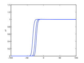
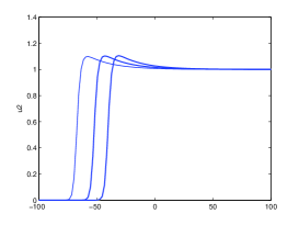
Figure 3: The simulations of the traveling wave solutions of (1.1). We choose $d_{1}=d_{2}=1,\kappa=0.05,\zeta=0.1,b=0.05$.

5 The Spreading Speed

5.1 Comparison Principle

We state the following comparison theorem for reaction-diffusion equations in File [9]. The comparison principle is a consequence of the maximum principle (see, e.g., Protter and Weingberger [13]). Another form of the comparison principle from [35] was used in [30]. As a result, the proof in Section 5 is somewhat different from [30]. By a suitable modification of the functions, the conditions in this paper seem easier to verify.

Theorem 5.1

Let $D$ be a positive definite diagonal matrix and $F=(F_{j})$ vector-valued continuous functions in $\mathbb{R}^{N}$. Assume that $F^{\pm}=(F_{j}^{\pm})$ are Lipschitz continuous on $\mathbb{R}$ and $F_{j}^{\pm}$ is nondecreasing in all but the $j$th component, $j=1,...,N$, and satisfying

$$F^{+}(u)\geq F(u)\geq F^{-}(u),u\in\mathbb{R}^{N}.$$

Let $u,u^{\pm}$ be continuous functions from $\mathbb{R}\times(0,T)$ into $\mathbb{R}^{N}$, $C^{2}$ in $\mathbb{R}\times(0,T)$, bounded and satisfying, for $i=1,...,n$

$$\begin{split}u_{t}-Du_{xx}&=F(u)\\ u^{+}_{t}-Du^{+}_{xx}&\geq F^{+}(u^{+})\\ u^{-}_{t}-Du^{-}_{xx}&\leq F^{-}(u^{-})\end{split}$$ (5.28)

If $u^{+}(x,t_{0})\geq u(x,t_{0})\geq u^{-}(x,t_{0}),\;\;x\in\mathbb{R}$, then

$$u^{+}(x,t)\geq u(x,t)\geq u^{-}(x,t),\;\;x\in\mathbb{R},t\in[t_{0},T].$$

We are now able to prove Parts (i) and (ii) of Theorem 3.1.

5.2 Proof of Parts (i) and (ii) of Theorem 3.1

Part (i). For a given $u_{0}\in\mathcal{C}_{k}$ with compact support, let $u^{+}(x,t)$ be the solutions of (2.5) with the same initial condition $u_{0}$, then Theorem 5.1 implies that $u^{+}(x,t)\in\mathcal{C}_{k^{+}}$ and

$$0\leq u(x,t)\leq u^{+}(x,t),x\in\mathbb{R},t>0.$$

Thus for any $c>c^{*}$, it follows from Theorem 2.2 (i) that

$$\lim_{t\to\infty}\sup_{\lvert x\rvert\geq tc}u^{+}(x,t)=0,$$

and hence

$$\lim_{t\to\infty}\sup_{\lvert x\rvert\geq tc}u(x,t)=0,$$

Part (ii). According to Theorem 2.2 (ii), for any strictly positive constant $\omega$, there is a positive $R_{\omega}$ (choose the larger one between the $R_{\omega}$ for (2.5) and the $R_{\omega}$ for (2.6)) with the property that if $u_{0}\geq\omega$ on an interval of length $2R_{\omega}$, then the solutions $u^{\pm}(x,t)$ of (2.5) and (2.6) with the same initial value $u_{0}$ are in $\mathcal{C}_{k^{+}}$ and satisfy

$$\liminf_{t\to\infty}\inf_{\lvert x\rvert\leq tc}u^{\pm}(x,t)=k^{\pm},\text{ for }0<c<c^{*}.$$

Thus, Theorem 5.1 implies that

$$u^{-}(x,t)\leq u(x,t)\leq u^{+}(x,t),x\in\mathbb{R},t>0.$$

Thus for any $c<c^{*}$, it follow from Theorem 2.2 (ii) that

$$\liminf_{t\to\infty}\inf_{\lvert x\rvert\leq ct}u^{\pm}(x,t)=k^{\pm},$$

and hence

$$k^{-}\leq\liminf_{t\to\infty}\inf_{\lvert x\rvert\leq ct}u(x,t)\leq k^{+}.$$

$\quad\Box$

6 The characterization of $c^{*}$ as the slowest speeds of traveling waves

6.1 Equivalent integral equations and their upper and lower solutions

In order to establish the existence of travel wave solutions, we fist set up equivalent integral equations. Similar equivalent integral equations were also used before, see for example, Wu and Zou [37], Ma [21, 22] and the author [28]. For the convenience of analysis, in this paper and [28], both $\lambda_{1i},\lambda_{2i}$ are chosen to be positive, and $-\lambda_{1i},\lambda_{2i}$ are solutions of (6.29).

Let $\beta>\max\{\lvert\partial_{i}f_{j}(x)\rvert,x\in[0,k^{+}],i,j=1,...,N\}>0.$ For $c>c^{*}$, the two solutions of the following equations,

$$d_{i}\lambda^{2}-c\lambda-\beta=0,i=1,...,N$$ (6.29)

are $-\lambda_{1i}$ and $\lambda_{2i}$ where

$$\lambda_{1i}=\frac{-c+\sqrt{c^{2}+4\beta d_{i}}}{2d_{i}}>0,\lambda_{2i}=\frac{c+\sqrt{c^{2}+4\beta d_{i}}}{2d_{i}}>0.$$

We choose $\beta$ sufficiently large so that

$$\lambda_{2i}>\lambda_{1i}>2\Lambda_{c},i=1,...,N.$$ (6.30)

Let $u=(u_{i})\in\mathcal{C}_{k}$ and define a operator $\mathcal{T}[u]=(\mathcal{T}_{i}[u])$ by

$$\begin{split}\mathcal{T}_{i}[u](\xi)&=\frac{1}{d_{i}(\lambda_{1i}+\lambda_{2i})}\Big{(}\int_{\infty}^{\xi}e^{-\lambda_{1i}(\xi-s)}H_{i}(u(s))ds\\ &\quad+\int^{\infty}_{\xi}e^{\lambda_{2i}(\xi-s)}H_{i}(u(s))ds\Big{)}\end{split}$$ (6.31)

where

$$H_{i}(u(s))=\beta u_{i}(s)+f_{i}(u(s)),$$

$\mathcal{T}_{i}[u],i=1,...,N$ is defined on $\mathbb{R}$ if $H_{i}(u),i=1,2$ is a bounded continuous function. In fact, the following identity holds

$$\begin{split}&\frac{1}{d_{i}(\lambda_{1i}+\lambda_{2i})}\big{(}\int_{-\infty}^{\xi}e^{-\lambda_{1i}(\xi-s)}\beta ds+\int^{\infty}_{\xi}e^{\lambda_{2i}(\xi-s)}\beta ds\big{)}\\ &=\frac{\beta}{d_{i}(\lambda_{1i}+\lambda_{2i})}\big{(}\frac{1}{\lambda_{1i}}+\frac{1}{\lambda_{2i}}\big{)}=\frac{\beta}{d_{i}(\lambda_{1i}\lambda_{2i})}\\ &=1.\end{split}$$ (6.32)

In fact, a fixed point $u$ of $\mathcal{T}$ or solution of the equation

$$u(\xi)=\mathcal{T}[u](\xi)\;\;\xi\in\mathbb{R},$$ (6.33)

is a traveling wave solution of (2.3) in Lemma 6.1. Lemma 6.1 summarizes the conclusion, which can be verified in the same manner as in [28] for scalar cases by directly substituting derivatives of $u(\xi)$ into (2.7). We omit its proof here.

Lemma 6.1

Assume $(H1-H2)$ hold. If $u\in\mathcal{C}_{k}$ is a fixed point of $\mathcal{T}[u]$,

$$u(\xi)=\mathcal{T}[u](\xi)\;\;\xi\in\mathbb{R},$$

then $u$ is a solution of (2.7).

We now define upper and lower solutions of (6.33), $\phi^{+}$ and $\phi^{-}$, which are only continuous on $\mathbb{R}$. Similar upper and lower solutions have been frequently used in the literatures. See Diekmann [7], Weinberger [34], Liu [18], Weinberger, Lewis and Li [31], Rass and Radcliffe [20], Weng and Zhao [36] and more recently, Ma [22], Fang and Zhao [8] and Wang [28, 29]. In particular, it is believed that the vector-valued lower solutions of the form in this paper first appeared in [36] for multi-type SIS epidemic models. In this paper, the upper and lower solutions here are defined and verified for the integral operator other than differential equations.

Definition 6.2

A bounded continuous function $u=(u_{i})\in C(\mathbb{R},[0,\infty)^{N})$ is an upper solution of (6.33) if

$$\mathcal{T}_{i}[u](\xi)\leq u_{i}(\xi),\;\;\text{for all }\xi\in\mathbb{R},i=1,...,N;$$

a bounded continuous function $u=(u_{i})\in C(\mathbb{R},[0,\infty)^{N})$ is a lower solution of (6.33) if

$$\mathcal{T}_{i}[u](\xi)\geq u_{i}(\xi),\;\;\text{for all }\xi\in\mathbb{R},i=1,...,N.$$

Let $c>c*$ and consider the positive eigenvalue $\Lambda_{c}$ and corresponding eigenvector $\nu_{\Lambda_{c}}=(\nu^{i}_{\Lambda_{c}})$, $\gamma$ in Lemma 2.1 and $q>1.$ Define

$$\phi^{+}(\xi)=(\phi^{+}_{i}),$$

where

$$\phi^{+}_{i}=\min\{k_{i},\nu^{i}_{\Lambda_{c}}e^{\Lambda_{c}\xi}\},i=1,...,N,\;\xi\in\mathbb{R};$$

and

$$\phi^{-}(\xi)=(\phi^{-}_{i}),$$

$$\phi^{-}_{i}=\max\{0,\nu^{i}_{\Lambda_{c}}e^{\Lambda_{c}\xi}-q\nu^{i}_{\gamma\Lambda_{c}}e^{\gamma\Lambda_{c}\xi}\},i=1,...,N,\;\xi\in\mathbb{R}.$$

It is clear that if $\xi\geq\frac{\ln\frac{k_{i}}{\nu^{i}_{\Lambda_{c}}}}{\Lambda_{c}}$, $\phi^{+}_{i}(\xi)=k_{i}$, and $\xi<\frac{\ln\frac{k_{i}}{\nu^{i}_{\Lambda_{c}}}}{\Lambda_{c}}$, $\phi^{+}_{i}(\xi)=\nu^{i}_{\Lambda_{c}}e^{\Lambda_{c}\xi},i=1,...,N.$

Similarly, if $\xi\geq\frac{\ln(q\frac{\nu^{i}_{\gamma\Lambda_{c}}}{\nu^{i}_{\Lambda_{c}}})}{(1-\gamma)\Lambda_{c}}$, $\phi^{-}_{i}(\xi)=0$, and for $\xi<\frac{\ln(q\frac{\nu^{i}_{\gamma\Lambda_{c}}}{\nu^{i}_{\Lambda_{c}}})}{(1-\gamma)\Lambda_{c}}$,

$$\phi^{-}_{i}(\xi)=\nu^{i}_{\Lambda_{c}}e^{\Lambda_{c}\xi}-q\nu^{i}_{\gamma\Lambda_{c}}e^{\gamma\Lambda_{c}\xi},i=1,...,N.$$

We choose $q>1$ large enough that

$$\frac{\ln(q\frac{\nu^{i}_{\gamma\Lambda_{c}}}{\nu^{i}_{\Lambda_{c}}})}{(1-\gamma)\Lambda_{c}}<\frac{\ln\frac{k_{i}}{\nu^{i}_{\Lambda_{c}}}}{\Lambda_{c}},i=1,...,N$$

and then

$$\phi^{+}_{i}(\xi)>\phi^{-}_{i}(\xi),i=1,...,N,\xi\in\mathbb{R}.$$

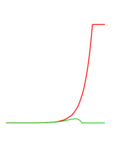
Figure 4: For each i, the curve above is $\phi^{+}_{i}$ and the below is $\phi^{-}_{i}$.

We now prove that $\phi^{+}$ and $\phi^{-}$ are upper and lower solution of (6.33) respectively.

Lemma 6.3

Assume $(H1)-(H2)$ hold and (2.3) is cooperative. For any $c>c^{*}$, $\phi^{+}$ defined above is an upper solution of (6.33).

[Proof.]Note that when (2.3) is cooperative, $f^{\pm}=f$ (see Remark 3.3). Let $\xi^{*}_{i}=\frac{\ln\frac{k_{i}}{\nu^{i}_{\Lambda_{c}}}}{\Lambda_{c}},i=1,...,N.$ We first need to verify that $u=(u_{i})=\phi^{+}$ is an upper solution of (2.7) in the sense that

$$d_{i}u^{\prime\prime}_{i}(\xi)-cu_{i}^{\prime}(\xi)+f_{i}(u(\xi))\leq 0,\;\;,i=1,...,N,\;\xi\neq\xi^{*}_{i}.$$ (6.34)

In view of the fact that $f_{i}(u(\xi))\leq f_{i}(k)=0$ for $\xi>\xi^{*}_{i}$, it is clear that (6.34) holds for $\xi>\xi^{*}_{i}$. For $\xi<\xi^{*}_{i}$, $u_{i}(\xi)=\nu^{i}_{\Lambda_{c}}e^{\Lambda_{c}\xi}$. From (H1-H2), we have, for $\xi<\xi^{*}_{i}$ and $i=1,...,N$

$$\begin{split}&d_{i}u_{i}^{\prime\prime}(\xi)-cu_{i}(\xi)+f_{i}(u(\xi))\\ &\leq d_{i}\Lambda_{c}^{2}\nu^{i}_{\Lambda_{c}}e^{\Lambda_{c}\xi}-c\Lambda_{c}\nu^{i}_{\Lambda_{c}}e^{\Lambda_{c}\xi}+\sum_{j=1}^{n}\partial_{j}f_{i}(0)\nu^{j}_{\Lambda_{c}}e^{\Lambda_{c}\xi}\\ &=\sum_{j=1}^{n}a^{ij}_{\Lambda_{c}}\nu^{j}_{\Lambda_{c}}e^{\Lambda_{c}\xi}-c\Lambda_{c}\nu^{i}_{\Lambda_{c}}e^{\Lambda_{c}\xi}\\ &=\Lambda_{c}\Phi(\Lambda_{c})\nu^{i}_{\Lambda_{c}}e^{\Lambda_{c}\xi}-c\Lambda_{c}\nu^{i}_{\Lambda_{c}}e^{\Lambda_{c}\xi}\\ &=0.\end{split}$$ (6.35)

Since $u^{\prime}_{i}(\xi^{*}-)\geq u^{\prime}_{i}(\xi^{*}+)=0$, the proof of Lemma 2.5 in Ma [21] immediately implies that

$$\mathcal{T}_{i}[u](\xi)\leq u_{i}(\xi),\;\;\text{for all }\xi\in\mathbb{R},i=1,...,N.$$

Thus $u=(u_{i})=\phi^{+}$ is an upper solution of (6.33). Note that the upper solutions in this paper are defined for equivalent integral equations other than differential equations in [21]. $\quad\Box$

We now need the following estimate on $f$, which is an application of the Taylor’s Theorem for multi-variable functions. Also see [28].

Lemma 6.4

Assume $(H1-H2)$ hold. There exist positive constants $b_{ij},i,j=1,...,N$ such that

$$f_{i}(u)\geq\sum_{j=1}^{N}\partial_{j}f_{i}(0)u_{j}-\sum_{j=1}^{N}b_{ij}(u_{j})^{2},\;\;u=(u_{i}),u_{i}\in[0,k_{i}],i=1,...,N.$$

Lemma 6.5

Assume $(H1)-(H2)$ hold. For any $c>c^{*}$, $\phi^{-}$ defined above is a lower solution of (6.33) if $q$ (which is independent of $\xi$) is sufficiently large.

[Proof.]Let Let $\xi^{*}_{i}=\frac{\ln(q\frac{\nu^{i}_{\gamma\Lambda_{c}}}{\nu^{i}_{\Lambda_{c}}})}{(1-\gamma)\Lambda_{c}},i=1,...,N.$ We first need to verify that $u=(u_{i})=\phi^{-}$ is a lower solution of (2.7) in the sense that

$$d_{i}u^{\prime\prime}_{i}(\xi)-cu_{i}^{\prime}(\xi)+f_{i}(u(\xi))\geq 0,\;\;\xi\neq\xi^{*}_{i},i=1,...,N.$$ (6.36)

It is clear that (6.36) holds for $\xi>\xi^{*}_{i}$. For $\xi<\xi^{*}_{i}$,

$$u_{i}(\xi)=\nu^{i}_{\Lambda_{c}}e^{\Lambda_{c}\xi}-q\nu^{i}_{\gamma\Lambda_{c}}e^{\gamma\Lambda_{c}\xi}<\nu^{i}_{\Lambda_{c}}e^{\Lambda_{c}\xi}.$$

From Lemma 6.4, we have, for $\xi<\xi^{*}_{i}$ and $i=1,...,N$

$$\begin{split}&d_{i}u_{i}^{\prime\prime}(\xi)-cu_{i}(\xi)+f_{i}(u(\xi))\\ &\geq d_{i}\Lambda_{c}^{2}\nu^{i}_{\Lambda_{c}}e^{\Lambda_{c}\xi}-c\Lambda_{c}\nu^{i}_{\Lambda_{c}}e^{\Lambda_{c}\xi}+\sum_{j=1}^{n}\partial_{j}f_{i}(0)\nu^{j}_{\Lambda_{c}}e^{\Lambda_{c}\xi}\\ &\quad-q\big{(}d_{i}(\gamma\Lambda_{c})^{2}\nu^{i}_{\gamma\Lambda_{c}}e^{\gamma\Lambda_{c}\xi}-c\gamma\Lambda_{c}\nu^{i}_{\gamma\Lambda_{c}}e^{\gamma\Lambda_{c}\xi}+\sum_{j=1}^{n}\partial_{j}f_{i}(0)\nu^{j}_{\gamma\Lambda_{c}}e^{\gamma\Lambda_{c}\xi}\big{)}\\ &\quad-\widehat{M}_{i}e^{2\Lambda_{c}\xi}\end{split}$$ (6.37)

where $\widehat{M}_{i}=\sum_{j=1}^{n}b_{ij}(\nu^{j}_{\Lambda_{c}})^{2}>0.$ Note that $e^{(2-\gamma)\Lambda_{c}\xi}$ is bounded above for $\xi\leq\xi_{i}$. With the same argument in (6.35), in particular, by Lemma 2.1, we get for sufficient large $q$ and $\xi\leq\xi_{i}$

$$\begin{split}&d_{i}u_{i}^{\prime\prime}(\xi)-cu_{i}(\xi)+f_{i}(u(\xi))\\ &\geq q\big{(}c\gamma\Lambda_{c}-\gamma\Lambda_{c}\Phi(\gamma\Lambda_{c})\big{)}\nu^{i}_{\gamma\Lambda_{c}}e^{\gamma\Lambda_{c}\xi}-\widehat{M}_{i}e^{2\Lambda_{c}\xi}\\ &=q\big{(}c-\Phi(\gamma\Lambda_{c})\big{)}\gamma\Lambda_{c}\nu^{i}_{\gamma\Lambda_{c}}e^{\gamma\Lambda_{c}\xi}-\widehat{M}_{i}e^{2\Lambda_{c}\xi}\\ &\geq\Big{(}q\big{(}c-\Phi(\gamma\Lambda_{c})\big{)}\gamma\Lambda_{c}\nu^{i}_{\gamma\Lambda_{c}}-\widehat{M}_{i}e^{(2-\gamma)\Lambda_{c}\xi}\Big{)}e^{\gamma\Lambda_{c}\xi}\\ &\geq 0.\end{split}$$ (6.38)

Since $u^{\prime}_{i}(\xi^{*}-)\leq u^{\prime}_{i}(\xi^{*}+)=0$, the proof of Lemma 2.6 in Ma [21] immediately implies that

$$\mathcal{T}_{i}[u](\xi)\geq u_{i}(\xi),\;\;\text{for all }\xi\in\mathbb{R},i=1,...,N.$$

Thus $u=(u_{i})=\phi^{+}$ is a lower solution of (6.33). Note that the upper solutions in this paper are defined for equivalent integral equations other than differential equations as in [21]. $\quad\Box$

.

6.2 Proof of Theorem 3.1 (iii) when (2.3) is cooperative

In this section, we assume that (2.3) is cooperative and prove Theorem 3.1 (iii). As we note in Remark 3.3, $f^{\pm}=f$. Many results in this section are standard. See, for example, Ma [21, 22] and Wang [28, 30]. Define the following Banach space

$$\mathcal{E}_{\varrho}=\{u=(u_{i}):u_{i}\in C(\mathbb{R}),\sup_{\xi\in\mathbb{R}}\lvert u_{i}(\xi)\rvert e^{-\varrho\xi}<\infty,i=1,...,N\}$$

equipped with weighted norm

$$\lVert u\rVert_{\varrho}=\sum_{i=1}^{N}\sup_{\xi\in\mathbb{R}}\lvert u_{i}(\xi)\rvert e^{-\varrho\xi},$$

where $C(\mathbb{R})$ is the set of all continuous functions on $\mathbb{R}$ and $\varrho$ is a positive constant such that $\varrho<\Lambda_{c}.$ It follows that $\phi^{+}\in\mathcal{E}_{\varrho}$ and $\phi^{-}\in\mathcal{E}_{\varrho}.$ Consider the following set

$$\mathcal{A}=\{u=(u_{i}):u_{i}\in C(\mathbb{R})\in\mathcal{E}_{\varrho},\phi_{i}^{-}(\xi)\leq u_{i}\leq\phi_{i}^{+}(\xi),\xi\in\mathbb{R},i=1,...,N.\}$$

We shall state the following lemmas. It is standard procedures to prove that $\mathcal{T}[u]$ is monotone, continuous and maps a bounded set in $\mathcal{A}$ into a compact set. We omit their proofs here. The proof of compactness can be carried out two steps. First we show that $\mathcal{T}$ is equicontinuous, and then Ascoli’s theorem and standard diagonal process can be used to prove that $\mathcal{T}$ is relatively compact $\mathcal{E}_{\varrho}.$ The proofs of Lemmas 6.6, 6.7, 6.8 are almost identical to those in [28, 30].

Lemma 6.6

Assume $(H1)-(H2)$ hold and $\partial_{i}f_{j}\geq 0,i\neq j$ on $[0,k]$. Then $\mathcal{T}$ defined in (6.31) is monotone and therefore $\mathcal{T}(\mathcal{A})\subseteq\mathcal{A}$. Furthermore, $\mathcal{T}_{i}[u]$ is nondecreasing if $u\in\mathcal{A}$ and all of $u_{i}$ are nondecreasing.

Lemma 6.7

Assume $(H1)-(H2)$ hold. Then $\mathcal{T}:\mathcal{A}\rightarrow\mathcal{E}_{\varrho}$ is continuous with the weighted norm $\lVert.\rVert_{\varrho}$.

Lemma 6.8

Assume $(H1)-(H2)$ hold. Then the set $\mathcal{T}(\mathcal{A})$ is relatively compact in $\mathcal{E}_{\varrho}.$

Now we are in a position to prove Theorem 3.1 when (2.3) is cooperative. Define the following iteration

$$u^{1}=(u_{i}^{1})=\mathcal{T}[\phi^{+}],\;\;u_{n+1}=(u_{i}^{n})=\mathcal{T}[u^{n}],n>1.$$ (6.39)

From Lemmas 6.3, 6.5, 6.6, $u_{n}$ is nondecreasing on $\mathbb{R}$ and

$$\phi_{i}^{-}(\xi)\leq u_{i}^{n+1}(\xi)\leq u_{i}^{n}(\xi)\leq\phi_{i}^{+}(\xi),\xi\in\mathbb{R},\;n\geq 1,n=1,...,N.$$

By Lemma 6.8 and monotonicity of ($u_{n}$), there is $u\in\mathcal{A}$ such that $\lim_{n\to\infty}\lVert u_{n}-u\rVert_{\varrho}=0$. Lemma 6.7 implies that $\mathcal{T}[u]=u$. Furthermore, $u$ is nondecreasing. It is clear that $\lim_{\xi\to-\infty}u_{i}(\xi)=0,i=1,...,N$. Assume that $\lim_{\xi\to\infty}u_{i}(\xi)=k_{i}^{\prime},i=1,...,N$ $k^{\prime}_{i}>0,i=1,...,N$ because of $u\in\mathcal{A}$. Applying the Dominated convergence theorem to (6.31), we get $k_{i}^{\prime}=\frac{1}{\beta}(\beta k_{i}^{\prime}+f_{i}(k_{1}^{\prime},...,k^{\prime}_{n})$ By (H1), $k_{i}^{\prime}=k_{i}$. Finally, note that

$$\nu^{i}_{\Lambda_{c}}(e^{\Lambda_{c}\xi}-q\e^{\gamma\Lambda_{c}\xi})\leq u_{i}(\xi)\leq\nu^{i}_{\Lambda_{c}}e^{\Lambda_{c}\xi},\xi\in\mathbb{R}.$$

We immediately obtain

$$\lim_{\xi\to-\infty}u_{i}(\xi)e^{-\Lambda_{c}\xi}=\nu^{i}_{\Lambda_{c}},i=1,...,N.$$ (6.40)

This completes the proof of Theorem 3.1 (iii) when (2.3) is cooperative.

6.3 Proof of Theorem 3.1 (iii)

[Proof.]Theorem 3.1 (iii) is proved when (2.3) is cooperative in the last section. Now we need to prove it in the general case(2.3) is not necessarily cooperative. In order to find traveling waves for (2.3), we will apply the Schauder’s fixed point theorem. Similar arguments can be found in the references, e.g. [22] and [30].

Let $u=(u_{i})\in\mathcal{A}$ and define two integral operators

$$\mathcal{T}^{\pm}[u]=(\mathcal{T}_{i}^{\pm}[u])$$

for $f^{-}$ and $f^{+}$

$$\begin{split}&\mathcal{T}_{i}^{\pm}[u](\xi)\\ &=\frac{1}{d_{i}(\lambda_{1i}+\lambda_{2i})}[\int_{-\infty}^{\xi}e^{-\lambda_{1i}(\xi-s)}H_{i}^{\pm}(u(s))ds+\int^{\infty}_{\xi}e^{\lambda_{2i}(\xi-s)}H_{i}^{\pm}(u(s))ds]\end{split}$$ (6.41)

and

$$H_{i}^{\pm}(u(s))=\beta u_{i}(s)+f_{i}^{\pm}(u_{(}s)).$$

As in Section 6.2, both $\mathcal{T}^{+}$ and $\mathcal{T}^{-}$ are monotone. In view of Section 6.2 and the fact that $f^{-}$ is nondecreasing, there exists a nondecreasing fixed point $u^{-}=(u_{i}^{-})$ of $\mathcal{T}^{-}$ such that $\mathcal{T}^{-}[u^{-}]=u^{-}$, $\lim_{\xi\to\infty}u_{i}^{-}(\xi)=k_{i}^{-},i=1,...,N$, and $\lim_{\xi\to-\infty}u_{i}^{-}(\xi)=0,i=1,...,N$. Furthermore, $\lim_{\xi\to-\infty}u_{i}^{-}(\xi)e^{-\Lambda_{c}\xi}=\nu^{i}_{\Lambda_{c}},i=1,...,N.$ According to Lemma 6.3, $\phi^{+}$ (with $k$ being replaced by $k^{\pm}$) is also a upper solution of $\mathcal{T}^{\pm}$ because the proof of Lemma 6.3 is still valid if $f$ is replaced by $f^{\pm}$. Let

$$\widetilde{\phi^{+}}(\xi)=(\widetilde{\phi^{+}_{i}}(\xi)),$$

where

$$\widetilde{\phi^{+}_{i}}(\xi)=\min\{k_{i}^{+},\nu^{i}_{\Lambda_{c}}e^{\Lambda_{c}\xi}\},i=1,...,N,\;\xi\in\mathbb{R};$$

It follows that $u_{i}^{-}(\xi)\leq\widetilde{\phi^{+}_{i}},\xi\in\mathbb{R},i=1,...,N.$ Now let

$$\mathcal{B}=\{u:u=(u_{i})\in\mathcal{E}_{\varrho},u_{i}^{-}(\xi)\leq u_{i}(\xi)\leq\widetilde{\phi^{+}_{i}}(\xi),\xi\in(-\infty,\infty),i=1,...,N\},$$ (6.42)

where $\mathcal{E}_{\varrho}$ is defined in Section 6.2. It is clear that $\mathcal{B}$ is a bounded nonempty closed convex subset in $\mathcal{E}_{\varrho}$. Furthermore, we have, for any $u=(u_{i})\in\mathcal{B}$

$$u_{i}^{-}=\mathcal{T}_{i}^{-}[u^{-}]\leq\mathcal{T}_{i}^{-}[u]\leq\mathcal{T}_{i}[u]\leq\mathcal{T}_{i}^{+}[u]\leq\mathcal{T}_{i}^{+}[\widetilde{\phi^{+}}]\leq\widetilde{\phi^{+}_{i}},i=1,...,N.$$

Therefore, $\mathcal{T}:\mathcal{B}\rightarrow\mathcal{B}$. Note that the proofs of Lemmas 6.7, 6.8 are valid if (2.3) is not cooperative. In the same way as in Lemmas 6.7, 6.8 , we can show that $\mathcal{T}:\mathcal{B}\rightarrow\mathcal{B}$ is continuous and maps bounded sets into compact sets. Therefore, the Schauder Fixed Point Theorem shows that the operator $\mathcal{T}$ has a fixed point $u$ in $\mathcal{B}$, which is a traveling wave solution of (2.3) for $c>c^{*}$. Since $u_{i}^{-}(\xi)\leq u_{i}(\xi)\leq\widetilde{\phi^{+}_{i}}(\xi),\xi\in(-\infty,\infty),i=1,...,N$, it is easy to see that for $i=1,...,N$, $\lim_{\xi\to-\infty}u_{i}(\xi)=0$, $\lim_{\xi\to-\infty}u_{i}(\xi)e^{-\Lambda_{c}\xi}=\nu^{i}_{\Lambda_{c}}$,

$$k^{-}\leq\liminf_{\xi\to\infty}u(\xi)\leq\limsup_{\xi\to\infty}u(\xi)\leq k^{+}$$

and $0<u_{i}^{-}(\xi)\leq u_{i}(\xi)\leq k_{i}^{+},\xi\in(-\infty,\infty)$. $\quad\Box$

6.4 Proof of Theorem 3.1 (iv)

[Proof.]We adopt the limiting approach in [3] to prove Theorem 3.1 (iv). For each $n\in\mathbb{N}$, choose $c_{n}>c^{*}$ such that $\lim_{n\to\infty}c_{n}=c^{*}.$ According to Theorem 3.1 (iii), for each $c_{n}$ there is a traveling wave solution $u_{n}=(u^{n}_{i})$ of (2.3) such that

$$u_{n}=\mathcal{T}[u_{n}](\xi).$$

and

$$k^{-}_{i}\leq\liminf_{\xi\to\infty}u^{n}_{i}(\xi)\leq\limsup_{\xi\to\infty}u^{n}_{i}(\xi)\leq k_{i}^{+},i=1,...,N.$$

It can be shown that $(u_{n})$ is equicontinuous and uniformly bounded on $\mathbb{R}$ (see, e.g. [28, Lemma 5.3]), the Ascoli’s theorem implies that there is vector valued continuous function $u=(u^{i})$ on $\mathbb{R}$ and subsequence $(u_{n_{m}})$ of $(u_{n})$ such that

$$\lim_{m\to\infty}u_{n_{m}}(\xi)=u(\xi)$$

uniformly in $\xi$ on any compact interval of $\mathbb{R}$. Further in view of the dominated convergence theorem we have

$$u=\mathcal{T}[u](\xi).$$

Here the underlying $\lambda_{1i},\lambda_{2i}$ of $\mathcal{T}$ is dependent on $c$ and continuous functions of $c$. Thus $u$ is a traveling solution of (2.3) for $c=c^{*}$. Since, for each $c_{n}$, $u_{n}\in\mathcal{B}$ where $\mathcal{B}$ is defined in (6.42), it is easy to see that $u$ satisfies

$$k^{-}\leq\liminf_{\xi\to\infty}u(\xi)\leq\limsup_{\xi\to\infty}u(\xi)\leq k^{+}$$

Because of the translation invariance of $u_{n}$, we always can assume that $u_{n}(0)\leq\frac{1}{2}k^{-}$ for all $n$. Consequently $u$ is not a constant traveling solution of (2.3). $\quad\Box$

6.5 Proof of Theorem 3.1 (v)

[Proof.]Suppose, by contradiction, that for some $c\in(0,c^{*})$, (2.3) has a traveling wave $u(x,t)=u(x+ct)$ with $\liminf_{\xi\to\infty}u(\xi)>>0$ and $u(-\infty)=0.$ Thus $u(x,t)=u(x+ct)$ can be larger than a positive vector with arbitrary length. It follows from Theorem 3.1 (ii)

$$\liminf_{t\to\infty}\inf_{\lvert x\rvert\leq ct}u(x,t)\geq k^{-}>>0,\text{ for }0<c<c^{*}$$

Let $\hat{c}\in(c,c^{*})$ and $x=\hat{c}t.$ Then

$$\lim_{t\to\infty}u\big{(}-(\hat{c}-c)t\big{)}=\lim_{t\to\infty}u(-\hat{c}t,t)\geq\liminf_{t\to\infty}\inf_{\lvert x\rvert\leq t\hat{c}}u(x,t)>>0.$$

However,

$$\lim_{t\to\infty}u\big{(}-(\hat{c}-c)t\big{)}=u(-\infty)=0,$$

which is a contradiction. $\quad\Box$

References

- [1] D. G. Aronson and H. F. Weinberger, Nonlinear diffusion in population genetics, combustion, and nerve pulse propagation, in Partial Differential Equations and Related Topics, J. A. Goldstein, ed., Lecture Notes in Mathematics Ser. 446, Springer-Verlag, Berlin, 1975, pp. 5-49.
- [2] D. G. Aronson and H. F. Weinberger, Multidimensional nonlinear diffusion arising in population dynamics, Adv. Math., 30 (1978), pp. 33-76.
- [3] K. Brown and J. Carr, Deterministic epidemic waves of critical velocity, Math. Proc. Cambridge Philos. Soc. 81 (1977) 431-433.
- [4] J. Cohen, Convexity of the dominant eigenvalue of an essentially non-negative matrix, Proc. Am. Math Soc. 81(1981) 675-658.
- [5] E.C.M. Crooks, On the Vol’pert theory of traveling-wave solutions for parabolic systems, Nonlinear Analysis 26 (1996) 1621-1642.
- [6] P.D. Dale, P.K. Maini, J.A. Sherratt, Mathematical modelling of corneal epithelial wound healing. Math. Biosci. 124 (1994) 127–147.
- [7] O. Diekmann, Thresholds and travelling waves for the geographical spread of an infection. J. Math. Biol. 6(1978) 109-130.
- [8] J. Fang and X. Zhao, MonotoneWavefronts for Partially Degenerate Reaction-Diffusion Systems, J. Dynam. Differential Equations 21 (2009) 663-680.
- [9] P. Fife, Mathematical aspects of reacting and diffusing systems. Lecture Notes in Biomathematics, 28. Springer-Verlag, Berlin-New York, 1979.
- [10] R. Fisher, The wave of advance of advantageous genes. Ann. of Eugenics, 7(1937) 355-369 .
- [11] R. Horn, C. Johnson, Matrix Analysis. Cambridge: University Press, Cambridge 1985
- [12] S. Hsu and X. Zhao, Spreading speeds and traveling waves for nonmonotone integrodifference equations, SIAM J. Math. Anal. 40(2008) 776-789.
- [13] M. Protter and H. Weinberger, Maximum principles in differential equations. Springer-Verlag, New York, 1984.
- [14] A. Kolmogorov, I. Petrovsky, N. Piscounoff, Etude de l equation de la diffusion avec croissance de la quantit e de mati‘ere et son application a un probl‘eme biologique. Bull. Moscow Univ. Math. Mech., 1(6), 1-26 (1937)
- [15] M. Lewis, B. Li and H. Weinberger, Spreading speed and linear determinacy for two-species competition models, Journal of Mathematical Biology, 45(2002) 219-233.
- [16] B. Li, H. Weinberger, M. Lewis, Spreading speeds as slowest wave speeds for cooperative systems. Math. Biosci. 196 (2005) 82-98.
- [17] B. Li, M. Lewis and H. Weinberger, Existence of traveling waves for integral recursions with nonmonotone growth functions, Journal of Mathematical Biology, 58(2009) 323-338.
- [18] R. Lui, Biological growth and spread modeled by systems of recursions. I. Mathematical theory. Math. Biosci. 93 (1989), no. 2, 269-295.
- [19] J. D. Murray, Mathematical Biology II: Spatial Models and Biomedical Applications, Springer-Verlag, New York, 2003.
- [20] L. Rass and J. Radcliffe, Spatial deterministic epidemics, Povidence, American Mathematical Society, 2003.
- [21] S. Ma, Traveling wavefronts for delayed reaction-diffusion systems via a fixed point theorem, J. Differential Equations, 171 (2001) 294-314.
- [22] S. Ma, Traveling waves for non-local delayed diffusion equations via auxiliary equation, Journal of Differential Equations, 237 (2007) 259-277.
- [23] J. Sherratt, J.D. Murray, Models of epidermal wound healing, Proc. R. Soc. London B 241 (1990) 29 -36.
- [24] J. Sherratt and J. Murray, Mathematical analysis of a basic model for epidermal wound healing, J. of Mathematical Biology, 29(1991) 389-404.
- [25] J. Smoller, Shock waves and reaction-diffusion equations, Springer-Verlag, New York, 1994.
- [26] H. R. Thieme, Density-Dependent Regulation of Spatially Distributed Populations and their Asymptotic speed of Spread. J. of Math. Biol., 8 (1979) 173-187.
- [27] A.I. Volpert, V.A. Volpert, V.A. Volpert, Traveling Wave Solutions of Parabolic Systems, Transl. Math. Monogr., vol. 140, Amer. Math. Soc., Providence, RI, 1994.
- [28] H. Wang, On the existence of traveling waves for delayed reaction-diffusion equations, Journal of Differential Equations, 247(2009) 887-905.
- [29] H. Wang, C. Castillo-Chavez, Spreading speeds and traveling waves for non-cooperative integro-difference systems, http://arxiv.org/abs/1003.1600.
- [30] H. Wang, Spreading speeds and traveling waves for non-cooperative reaction-diffusion systems, http://arxiv.org/abs/1007.0950.
- [31] H. F. Weinberger, M. A. Lewis and B. Li, Analysis of linear determinacy for spread in cooperative models, J. Math. Biol. 45(2002) 183-218.
- [32] H. F. Weinberger, M. A. Lewis and B. Li, Anomalous spreading speeds of cooperative recursion systems, J. Math. Biol. 55(2007) 207-222.
- [33] H. F. Weinberger, Long-time behavior of a class of biological models. SIAM J. Math. Anal., 13 (1982) 353-396.
- [34] H. F. Weinberger, Asymptotic behavior of a model in population genetics. In Nonlinear Partial Differential Equations and Applications, ed. J. M. Chadam Lecture Notes in Mathematics, Volume 648, pages 47-96. Springer-Verlag, Berlin, 1978.
- [35] H. F. Weinberger, K. Kawasaki and N. Shigesada, Spreading speeds for a partially cooperative 2-species reaction-diffusion model, discrete and continuous dynamical systems, 23(2009), 1087-1098.
- [36] P. Weng, X, Zhao, Spreading speed and traveling waves for a multi-type SIS epidemic model, Journal of Differential Equations, 229(2006) 270-296.
- [37] J. Wu, X. Zou, Traveling wave fronts of reaction diffusion systems with delay, J. Dynam. Differential Equations 13 (2001) 651-687.