Abstract

We construct the spectrum generating algebra (SGA) for a free particle in the three dimensional sphere $S^{3}$ for both, classical and quantum descriptions. In the classical approach, the SGA supplies time-dependent constants of motion that allow to solve algebraically the motion. In the quantum case, the SGA include the ladder operators that give the eigenstates of the free Hamiltonian. We study this quantum case from two equivalent points of view.

1 Introduction

The notion of spectrum generating algebra (SGA), sometimes called non invariance algebra, was introduced many years ago [1, 2, 3]. In the context of quantum mechanics, the idea of the SGA consists in reducing the construction of the whole Hilbert space for a given system to a problem of representation theory. The knowledge of the symmetry (usually called ‘dynamical symmetry’) of a problem allows to solve it only partly: its representations gives the subspace of the whole Hilbert space of eigenstates corresponding to a fixed energy. The further extension to the SGA needs to introduce ladder operators that change the energy, i.e., operators that do not commute with the Hamiltonian (it is the reason to call this construction non-invariance algebra). At the very best, the whole set of operators —those generating the dynamical algebra plus the ladder operators— may form a finite dimensional non-compact algebra whose representation gives the Hilbert space of the system. In this respect, the symmetry algebra of the Hamiltonian plays the role of the Cartan subalgebra, while the additional operators of the SGA, which do not commute with the Hamiltonian, play the role of the Borel elements.

In the classical frame, the symmetry algebra provides constants of motion which are functions of the dynamical variables characterizing the possible trajectories. However, the motion is obtained from another kind of constants of motion that include explicitly the time. Such constants come from the elements of the SGA ‘not commuting’ (in the sense of Poisson brackets) with the Hamiltonian [5].

The main purpose of this paper is using the SGA technique to solve the spectral problem related with the quantum Hamiltonian of the free motion in the three dimensional sphere $S^{3}$, embedded in the four dimensional coordinate space ${\mathbb{R}}^{4}$, which has a pure discrete spectrum [4]. This problem is already nontrivial, interesting by itself and will provide important clues for the extension of the SGA in the study of more general quantum systems evolving on configuration spaces with constant curvature. In the case of the free particle in $S^{3}$, it is well known that the symmetry algebra is $\mathfrak{so}(4)$ and our task is to construct the ladder operators which do not commute with the Hamiltonian. As we shall see below in order to achieve this goal we will need to involve, apart from symmetry operators, also the elements of the homogenous space of the group $SO(4)$. The main result obtained in this work is the explicit construction of a SGA isomorphic to $\mathfrak{so}(4,2)$.

It is interesting to remark that this is a new method to study classical and quantum systems in configuration spaces of nonzero constant curvature. However, the study of such systems is not new up to the extent that Schrödinger himself has obtain the levels of energy of the Kepler problem in $S^{3}$, see [4]. For other approaches, see [6, 7].

The paper is organized as follows. Section 2 begins with the construction of the SGA for the free particle in $S^{3}$ in the classical context. This is a good starting point, as it will give us hints for the construction of the quantum SGA of the same problem. However, the classical version is much simpler, as is free of the important and hampering difficulties of the ordering of non-commuting operators, which is specific of the quantum case. In this section we will also show how we can use the SGA in order to solve the classical equations of motion. In section 3, we shall present the detailed construction of the SGA for the quantum problem. Here, we have adopted the point of view of a direct quantization of the classical SGA and choose the representation by means of some natural restrictive relations. The Hilbert space of states will be explicitly derived with the help of the SGA through ladder operators. At the very end, we obtain position and momentum operators along to constraint and gauge fixing relations compatible with $S^{3}$. In Section 4, we adopt the opposite point of view. We start with canonical quantizations of the classical Dirac brackets for the variables position and momentum with their corresponding constraint and gauge condition compatible with $S^{3}$. Then determine the SGA, as well as the ladder operators. We also derive the restrictive relations as a consequence of our definitions. Finally, we present the concluding remarks and some indications for future research.

2 The classical case

We shall start with the Lagrangian of the free motion in $S^{3}$, considered as a sphere of radius one,

$$L=\frac{1}{8{\bf x}^{4}}\;\sum_{i,j=1}^{4}(x_{i}\dot{x}_{j}-\dot{x}_{i}x_{j})^{2}\,,\quad{\rm with}\qquad{\bf x}^{2}=\sum_{i=1}^{4}x_{i}^{2}\,,$$ (1)

where the dot represents the derivative with respect to time and we have assumed $m=1$, since the mass do not play any relevant role in our development. This Lagrangian can be considered the restriction to the sphere $S^{3}$ of the free Lagrangian $L=\sum_{i=1}^{4}\dot{x}_{i}^{2}$ defined in the ambient space ${\mathbb{R}}^{4}$. The canonical momenta are determined by

$$p_{i}=\frac{\partial L}{\partial\dot{x}_{i}}=\frac{1}{2{\bf x}^{4}}\;\sum_{j=1}^{4}(x_{j}\dot{x}_{i}-x_{i}\dot{x}_{j})x_{j}\,,$$ (2)

and satisfies the primary constraint

$${\bf x}{\bf p}=x_{i}p_{i}=0\,,$$ (3)

${\bf x}{\bf p}=x_{i}p_{i}=0$, where here and throughout the paper the convention of summation over repeated indices is used (in this respect, Latin subindexes $i,j,k,\dots$ will run from $1$ to $4$, the dimension of the ambient space).

The Legendre transformation of the Lagrangian (1) gives the canonical Hamiltonian

$$H=\frac{1}{2}\;J_{ij}J_{ij}\,,\qquad J_{ij}=x_{i}p_{j}-x_{j}p_{i}\,,$$ (4)

where $J_{ij}$ has the structure of an angular momentum. Our strategy to work in $S^{3}$ will be the following. Instead of dealing in the 8-dimensional phase space with dynamical variables $x_{i},p_{i}$ satisfying the canonical Poisson brackets, we impose the gauge fixing condition

$${\bf x}^{2}=x_{i}x_{i}=1,$$ (5)

and the primary constrain (3). According to the usual procedure [10, 11], we also introduce the Dirac brackets

$$\{x_{i},x_{j}\}_{D}=0\,,\quad\{p_{i},x_{j}\}_{D}=\delta_{ij}-x_{i}x_{j}\,,\quad\{p_{i},p_{j}\}_{D}=J_{ij}\,.$$ (6)

In the sequel, we prefer to use the variables $x_{i}$ and $p_{i}$ subject to the Dirac brackets (6) instead of defining a set of independent variables in $S^{3}$, because this would lead us to very complicated expressions. Therefore, from now on, as we will work in the configuration space $S^{3}$ where only Dirac brackets will be appropriate, the label $D$ (such as it appears in (6)) will be suppressed.

It is interesting to remark in passing that we can supply a realization of the variables $x_{i}$, $p_{j}$ in terms of canonical variables and the usual Poisson brackets. Let us consider the canonical variables $\xi_{i},\pi_{j}$, $i=1,\dots,4$, and the associated Poisson brackets,

$$\{\phi,\psi\}_{P}=\sum_{i}\left(\frac{\partial\phi}{\partial\pi_{i}}\frac{\partial\psi}{\partial\xi_{i}}-\frac{\partial\psi}{\partial\pi_{i}}\frac{\partial\phi}{\partial\xi_{i}}\right)\,.$$ (7)

Then, let us define the following relations

$$x_{i}({\boldsymbol{\xi}},{\boldsymbol{\pi}}):=\frac{\xi_{i}}{\xi},\quad p_{i}({\boldsymbol{\xi}},{\boldsymbol{\pi}}):=\xi\pi_{i}-({\boldsymbol{\pi}}{\boldsymbol{\xi}})\frac{\xi_{i}}{\xi^{2}},\quad\textstyle\xi=\sqrt{\sum_{k}(\xi_{k})^{2}}\,,$$ (8)

and also Dirac brackets by

$$\{f({\bf x},{\bf p}),g({\bf x},{\bf p})\}_{D}:=\{f({\boldsymbol{\xi}},{\boldsymbol{\pi}}),g({\boldsymbol{\xi}},{\boldsymbol{\pi}})\}_{P}\,$$ (9)

where in the last expression the functions depending on ${\boldsymbol{\xi}},{\boldsymbol{\pi}}$ have been obtained by the replacement of ${\bf x},{\bf p}$ given in (8). Then, (8), (9) gives us the desired representation.

From now on, we shall consider Dirac brackets only, so that the subindex $D$ in brackets like (6) will be omitted in the sequel.

The components $J_{ij}$ of the angular momentum introduced in (3) satisfy the following ‘commutation’ relations:

$$\{J_{ik},J_{lm}\} = \delta_{im}J_{kl}+\delta_{kl}J_{im}-\delta_{il}J_{km}-\delta_{km}J_{il}\,,$$ (10)

$$\{J_{ik},x_{l}\} = \delta_{lk}x_{i}-\delta_{il}x_{k}\,,$$ (11)

$$\{J_{ik},p_{l}\} = \delta_{lk}p_{i}-\delta_{il}p_{k}\,,$$ (12)

which coincide with those well known using canonical Poisson brackets. Hence, the elements $J_{ij}$ are the generators of the Lie algebra $\mathfrak{so}(4)$ of the group $SO(4)$. This Lie algebra has two Casimirs:

$$H = \frac{1}{2}\;J_{ij}J_{ij}={\bf p}^{2}{\bf x}^{2}-(\bf{xp})^{2}={\bf p}^{2}\,,$$ (13)

$$C_{2} = \epsilon_{ijkl}J_{ij}J_{kl}=\bf{xp}=0\,.$$ (14)

Thus, the only nontrivial Casimir plays the role of the Hamiltonian $H$ and it can be seen as the restriction to $S^{3}$ of the free Hamiltonian defined in the ambient space. Consequently, the symmetry algebra is just $\mathfrak{so}(4)$ itself, but taking into account that this symmetry is realized by a representation in which the second Casimir (14) vanishes.

In the rest of this section we will show that what can be called the ‘classical’ SGA for this system has the structure of the $\mathfrak{so}(4,2)$ algebra, including the aforementioned realization of $\mathfrak{so}(4)$ as a subalgebra.

The generators of the Lie algebra $\mathfrak{so}(4,2)$ will be labeled $M_{\alpha\beta}$ with $\alpha,\beta=1,\dots,6$. They include the generators of the symmetry algebra in the form $M_{ij}=J_{ij}$. The new generators completing the ‘classical’ SGA are $M_{5i}$ and $M_{6i}$, that behave as vectors with respect to $SO(4)$ and $M_{56}$ which is an $SO(4)$–scalar. These generators can be displayed schematically in the form of a $6\times 6$ antisymmetric matrix as follows:

$$M_{\alpha\beta}=\left(\begin{array}[]{cc}J_{ij}&\begin{array}[]{ccc}M_{i5}&M_{i6}\end{array}\\[4.30554pt] \begin{array}[]{c}M_{5i}\\[4.30554pt] M_{6i}\end{array}&\begin{array}[]{cc}0&M_{56}\\[4.30554pt] M_{65}&0\end{array}\\ \end{array}\right)\,,$$ (15)

such that $M_{\alpha\beta}=-M_{\beta\alpha}$. The $\mathfrak{so}(4,2)$ ‘commutation’ relations (in the sense of Dirac brackets) are

$$\{M_{\alpha\beta},M_{\gamma\delta}\}=g_{\alpha\delta}M_{\beta\gamma}+g_{\beta\gamma}M_{\alpha\delta}-g_{\alpha\gamma}M_{\beta\delta}-g_{\beta\delta}M_{\alpha\gamma}\,,$$ (16)

where $g_{\alpha\beta}$ is the metric matrix for $SO(4,2)$, given by the diagonal $6\times 6$ matrix $(1,1,1,1,-1,-1)$. In the following, we will pay special attention to the commutators of the generators not belonging to $\mathfrak{so}(4)$:

$$\{M_{i5},M_{56}\} = -M_{i6}\,,$$ (17)

$$\{M_{i6},M_{56}\} = M_{i5}\,,$$ (18)

$$\{M_{i5},M_{k6}\} = -\delta_{ik}M_{56}\,,$$ (19)

$$\{M_{i5},M_{k5}\} = J_{ik}\,,$$ (20)

$$\{M_{i6},M_{k6}\} = J_{ik}\,.$$ (21)

Our next objective is to calculate explicit expressions for $M_{5i},M_{6i},M_{56}$ implementing these commutators. In this process we need two $SO(4)$ vectors and one $SO(4)$ scalar. From (11) and (12), the vectors at hand are $\bf{x}$ and $\bf{p}$, while the scalar is just $H$, therefore we can make the following guess for these generators:

$$M_{i5}=p_{i}f_{5}(H),\quad M_{i6}=x_{i}f_{6}(H),\quad M_{56}=f_{56}(H)$$ (22)

where $f_{5},f_{6},f_{56}$ are functions to be determined. Remark that due to the specific realization we have

$$p_{i}=-J_{ik}x_{k}\,.$$ (23)

Since the Dirac brackets for $p_{i}$ in $S^{3}$ are not familiar (see (6)), we prefer to use the equivalent expression (23), because its factors obey the Dirac brackets with the familiar form (6)–(11). The final solution in this classical frame can be easily obtained:

$$M_{i5}=J_{ik}x_{k},\quad M_{i6}=H^{1/2}x_{i},\quad M_{56}=H^{1/2}\,.$$ (24)

Making use of the ‘classical’ SGA, we can solve the equation of motion for the present case. To this end, let us introduce the functions $A_{j}^{\pm}$ as the following linear combinations of $M_{5i}$ and $M_{6i}$:

$$A_{j}^{\pm}:=M_{5j}\mp iM_{6j}\,,\qquad j=1,\dots 4\,.$$ (25)

The importance of the $SO(4)$ vectors $A_{j}^{\pm}$ will have quite different implications in the classical and quantum cases. Clearly, the equations of motion for $A_{j}^{\pm}$ are given by

$$\dot{A}_{j}^{\pm}=\{H,A_{j}^{\pm}\}=2\sqrt{H}\{\sqrt{H},A_{j}^{\pm}\}=\pm 2\sqrt{H}\,iA_{j}^{\pm}\,,$$ (26)

where the dot denotes derivative with respect time. Then, (26) gives:

$$A_{j}^{\pm}(t)=\exp\{\pm 2i\,t\sqrt{H}\}\,A_{j}^{\pm}(0)\,,$$ (27)

which provide the motion $(x_{j}(t),p_{j}(t))$. Notice that the frequency $\omega=2\sqrt{H}$ depends on $H$ and increases as the system has higher energies. Another way to express (27) is to say that $A_{j}^{\pm}(t)\exp\{\mp 2it\sqrt{H}\}$ are time-dependent constants of motion whose values $A_{j}^{\pm}(0)$ are fixed from the initial conditions. Therefore, the symmetries lead to (time-independent) constants of motion, while the other SGA elements lead in this way to explicit time-dependent constants of motion giving the motion.

On the other hand, $A^{+}_{i}A^{-}_{i}$ is a time-independent $SO(4)$ scalar function, that can be computed explicitly:

$$A^{+}_{i}A^{-}_{i}=A^{+}_{i}(0)A^{-}_{i}(0)=2H\,,$$ (28)

so that the amplitudes $|A_{i}^{\pm}(0)|$ in (27) also depend on the Hamiltonian. We can also compute the value of the quadratic Casimir of $\mathfrak{so}(4,2)$ with the help of (28):

$$M^{\alpha\beta}M_{\alpha\beta}=J_{ij}J_{ij}+2M_{56}^{2}-2(M_{5i}M_{5i}+M_{6i}M_{6i})=2H+2H-2(2H)=0\,.$$ (29)

We see that (29) also gives (28).

As a final remark, we shall note that some restrictive relations among the algebra generators are fulfilled. These relations will have a crucial role in the construction of the quantum SGA for the quantum case. In fact, a rather straightforward calculation show that the tensors given by

$$T_{ab}:=M_{ac}M_{bd}\,g^{cd}\qquad{\rm and}\qquad R^{ab}:=\varepsilon^{abcdef}\,M_{cd}M_{ef}\,,$$ (30)

where $\varepsilon^{abcdef}$ is the complete antisymmetric tensor, vanish identically, i.e.,

$$T_{ab}=0\qquad{\rm and}\qquad R^{ab}=0\,.$$ (31)

We shall call relations (31) restrictive relations for the algebra ${\mathfrak{s}o}(4,2)$. These relations are not changed under the action of the algebra since a direct calculation using (16) gives:

$$\{M_{ab},T_{cd}\}=g_{ac}\,T_{bd}-g_{bc}\,T_{ad}+g_{ad}\,T_{cb}-g_{bd}\,T_{ca}\,.$$ (32)

A similar relation holds for $\{M_{ab},R^{cd}\}$.

Here, we conclude the discussion of the classical SGA for $S^{3}$.

3 The Quantum Case

Let us analyze the quantized version of the discussion given in the previous section. We shall adopt a point of view of starting with the quantized version of (16). In any case and by analogy with the classical case, we shall work in a realization in which the Casimirs for the symmetry algebra $\mathfrak{so}(4)$ are the free Hamiltonian

$$H=\frac{1}{2}\,J_{jk}J_{jk}$$ (33)

and

$$C_{2}=\frac{1}{2}\epsilon_{ijkl}J_{ij}J_{kl}=0\,.$$ (34)

We shall present the discussion of the quantum case in the next following subsections.

3.1 The symmetry algebra

The symmetry algebra of $H$ is clearly determined by the operators $J_{jk}$ that close the algebra $\mathfrak{so}(4)$. We recall (see for instance [12]) that the algebra $\mathfrak{so}(4)$ is the direct sum of two copies of $\mathfrak{su}(2)$, i.e., $\mathfrak{so}(4)=\mathfrak{su}(2)\oplus\mathfrak{su}(2)$. If we group the six generators $J_{jk}$ as the components of two vectors $\bf{R}=(J_{23},-J_{13},J_{12})$ and $\bf{S}=(J_{14},J_{24},J_{34})$, then the generators of each copy of $\mathfrak{su}(2)$ are given by $\bf{M}=(\bf{R}+\bf{S}$)/2 and $\bf{N}=(\bf{R}-\bf{S})/2$, respectively. The corresponding $\mathfrak{su}(2)$ Casimirs are $\bf{M}^{2}=(\bf{R}+\bf{S})^{2}/4=(\bf{R}^{2}+\bf{R}\bf{S}+\bf{S}\bf{R}+\bf{S}^{2})/4$, and $\bf{N}^{2}=(\bf{R}-\bf{S})^{2}/4=(\bf{R}^{2}-\bf{R}\bf{S}-\bf{S}\bf{R}+\bf{S}^{2})/4$ . Thus, the Hamiltonian in (LABEL:28) can be expressed in the form

$$H=2(\bf{M}^{2}+\bf{N}^{2})$$ (35)

The Hilbert space spanned by the states with the same energy support a unitary irreducible representation (UIR) of $SO(4)$. However, we must take into account that in this particular realization we have that ${\bf RS}+{\bf SR}=C_{2}=\frac{1}{2}\epsilon_{ijkl}J_{ij}J_{kl}=0$, so that the value for both of the Casimirs for $\mathfrak{su}(2)$ coincides: $\bf{M}^{2}=\bf{N}^{2}=j(j+1)$ with $j=0,1/2,1,3/2,\dots$. Then, each representation supported by states with the same energy is symmetric and hence the spectrum of the Hamiltonian is given by

$${\rm Spec}(H)=4j(j+1)=n(n+2),\qquad n=0,1,\dots$$ (36)

The $n$-th energy level has the value $j=n/2$ for each of the $\mathfrak{su}(2)$–components, and consequently the degeneracy of this energy level is $(n+1)^{2}$.

3.2 The quantum Spectrum Generating Algebra.

To begin with, let us take the quantized version of formula (16). This quantized formula gives us the relation between the generators of $SO(4,2)$, where these generators are operators on a certain Hilbert space and the Dirac brackets have been replaced by commutators. It reads:

$$[M_{ab},M_{cd}]=-i(g_{ad}M_{bc}+g_{bc}M_{ad}-g_{ac}M_{bd}-g_{bd}M_{ac})\,,$$ (37)

with $a,b=1,\dots,6$ and $\{g_{ab}\}$ is a $6\times 6$ diagonal matrix with diagonal $(1,1,1,1,-1,-1)$. Take the indices $i,j=1,2,3,4$ and introduce the following notation:

$$M_{ij}=J_{ij},\quad M_{i5}=K_{i},\quad M_{i6}=L_{i},\quad M_{56}=h\,.$$ (38)

We use this notation (38) in formula (37) so as to obtain

$$[J_{ik},J_{lm}]=-i(\delta_{im}J_{kl}+\delta_{kl}J_{im}-\delta_{il}J_{km}-\delta_{km}J_{il})$$

$$[J_{ik},K_{l}]=-i(\delta_{kl}K_{i}-\delta_{il}K_{k}),\quad[J_{ik},L_{l}]=-i(\delta_{kl}L_{i}-\delta_{il}L_{k})$$

$$[K_{i},K_{j}]=[L_{i},L_{j}]=-iJ_{ij},\quad[K_{i},L_{j}]=i\delta_{ij}h$$

$$[K_{i},h]=iL_{i},\quad[L_{i},h]=-iK_{i}\,.$$ (39)

One of the important features of the SGA are the ladder operators which will be used in order to construct the Hilbert space of pure states of the system. By close analogy with the classical case (see equation (25)), we define

$$A^{\pm}_{i}=K_{i}\mp iL_{i}\,,\qquad i=1,2,3,4\,.$$ (40)

These operators behave as vectors with respect to the generators $J_{ij}$ of the algebra $\mathfrak{so}(4)$, as shown in the second row of (39). They satisfy the following commutation relations:

$$[A^{+}_{i},A^{-}_{j}]=-2iJ_{ij}-2\delta_{ij}h,\quad[A^{+}_{i},A^{+}_{j}]=[A^{-}_{i},A^{-}_{j}]=0,$$

$$hA^{+}_{i}=A^{+}_{i}(h+1),\quad hA^{-}_{i}=A^{-}_{i}(h-1)\,.$$ (41)

Now, our purpose is to identify the quantum system with spectrum generating algebra given by $SO(4,2)$. In order to accomplish this, we need to find some restrictive relations for the generators of the algebra $\mathfrak{so}(4,2)$. This reflect the fact that, in general, the Hilbert space obtained with this technique is not the Hilbert space which supports a general representation of $SO(4,2)$. This kind of restrictive relations is very well known, although not very well identified often.

In order to understand this fact, let us consider the simple example of $SO(3)$. Its generators satisfy the familiar commutation relations

$$[S_{i},S_{j}]=i\epsilon_{ijk}S_{k}\,.$$ (42)

The representations of $SO(3)$ are well known and are labelled by the eigenvalues $s$ of the Casimir operator. At the same time, we can impose on the generators $S_{i}$ some additional conditions. For instance:

$$T_{ij}=S_{i}S_{j}+S_{j}S_{i}-\frac{1}{2}\,\delta_{ij}=0\,,$$ (43)

which are compatible with (42). In fact,

$$[S_{l},T_{ij}]=i(\epsilon_{lik}T_{kj}+\epsilon_{lij}T_{ik})\,.$$ (44)

Condition (43) is a restrictive relation of the mentioned type. Then, if in the space supporting all representations of $SO(3)$, we are to define a subspace $V$ satisfying the condition $T_{ij}\psi=0$, the action of the generators of $SO(3)$ on $V$ should not leave $V$. In the chosen example, it becomes clear that the space in which this condition is satisfied corresponds to the choice of $s=1/2$. For higher values of the spin, the restrictive relations for $SO(3)$ involve higher powers of $S_{i}$.

In the case of a non compact algebra like $\mathfrak{so}(4,2)$, the situation is more complicated so that even a quadratic restriction relation may define a subspace $V$ of infinite dimension. Thus, the first problem that we have to solve is to find a general expression for the restrictive relations concerning $SO(4,2)$. These restrictive relations will be given by operators (as in (43) such that their commutators with the generators $M_{ab}$ are linear on these operators. This task is not difficult if we construct the operators providing the restrictive relations as tensors constructed from $M_{ab}$.

One more remark is in order here. As we have seen in the classical case, all generators of $SO(4,2)$ (6+4+4+1=15), were build by using $x_{i}$ and $p_{i}$. This shows the existence of some relations between the $M_{ab}$. In the quantum case, these relations cannot be valid in the general representation of $SO(4,2)$, but they may hold for particular representations and this is the case here.

To produce this construction, let us go back to tensors (30). In our representation we have changed the meaning of the objects $M_{ab}$ that do not represent functions any more like in (30), but Hermitian operators instead. Since these operators do not commute, we have to symmetrize (30) so that the new expression for $T_{ab}$ should be given by

$$T_{ab}=(M_{ad}M_{be}+M_{be}M_{ad})g^{de}\,,$$ (45)

which is covariant with respect to the generators of $SO(4,2)$:

$$[M_{ab},T_{cd}]=i(g_{ac}T_{bd}-g_{bc}T_{ad}+g_{ad}T_{cb}-g_{bd}T_{ca})\,.$$ (46)

Needless to say that (46) replaces (32) in the present discussion. Moreover, if we add a constant term $cg_{ab}$, where $c$ is arbitrary, to $T_{ab}$:

$$\widetilde{T}_{ab}=T_{ab}+cg_{ab}\,,$$ (47)

then, $\widetilde{T}_{ab}$ will satisfy the same equation.

A second restrictive relation is given by the following tensor, which is clearly the quantized version of the second tensor in (30):

$$R^{ab}=\epsilon^{abcdef}(M_{cd}M_{ef}+M_{ef}M_{cd})\,.$$ (48)

Then, we need to express the components of $\widetilde{T}_{ab}$ and $R_{ab}$ in terms of the components $M_{ab}$. We shall do it using the notation introduced in (38). The components of $T_{ab}$ are

$$\widetilde{T}_{ij}=J_{ik}J_{jk}+J_{jk}J_{ik}-(K_{i}K_{j}+K_{j}K_{i}+L_{i}L_{j}+L_{j}L_{i})+cg_{ij}\,,$$ (49)

$$\widetilde{T}_{5i}=-(hL_{i}+L_{i}h)-(J_{ij}K_{j}+K_{j}J_{ij})\,,$$ (50)

$$\widetilde{T}_{6i}=hK_{i}+K_{i}h-(J_{ij}L_{j}+L_{j}J_{ij})\,,$$ (51)

$$\widetilde{T}_{56}=K_{i}L_{i}+L_{i}K_{i}\,,$$ (52)

$$\widetilde{T}_{55}=2(K_{i}^{2}-h^{2})-c\,,$$ (53)

$$\widetilde{T}_{66}=2(L_{i}^{2}-h^{2})-c\,.$$ (54)

Also note that we are using the convention of sum over repeated indices. This is also true in (53) and (54), where we have the terms $L_{i}^{2}=L_{i}L_{i}=\sum_{i=1}^{4}L_{i}^{2}$ and also $K_{i}^{2}=K_{i}K_{i}=\sum_{i=1}^{4}K_{i}^{2}$. We shall use this convention from now on. For instance, $X_{i}^{2}$ will denote $\sum_{i=1}^{n}X_{i}^{2}$, etc.

The components of $R^{ab}$ are

$$R^{ij}=K_{i}L_{j}+L_{j}K_{i}-(L_{i}K_{j}+K_{j}L_{i})-2hJ_{ij}\,,$$ (55)

$$R^{5i}=\epsilon_{ijkl}(L_{j}J_{kl}+J_{kl}L_{j})\,,$$ (56)

$$R^{6i}=\epsilon_{ijkl}(K_{j}J_{kl}+J_{kl}K_{j})\,,$$ (57)

$$R^{56}=\epsilon_{ijkl}J_{ij}J_{kl}\,.$$ (58)

Once we have defined the operators giving the restriction relations, we can write these relations as:

$$\widetilde{T}_{ab}=0,\qquad R^{ab}=0\,.$$ (59)

The next step is finding operators that can play the role of position operators. Thus, we find four operators $X_{i}$, $i=1,2,3,4$ subject to these conditions: i.) the operators $X_{i}$ commute with each other and ii.) $X_{i}^{2}=1$, i.e., they determine the position on the sphere $S^{3}$. We have the following Ansatz for the $X_{i}$:

$$X_{i}=f(h)A^{+}_{i}+g(h)A^{-}_{i}\,.$$ (60)

This Ansatz is motivated by the fact that $X_{i}$ should behave as a vector with respect to the representations of $SO(4)$. Vectors with respect these representations are those with components $L_{i}$ and $K_{i}$ only. These vectors are linear combinations of $A_{i}^{\pm}$. The most general linear combination of these operators is given by (60) since $h$ behaves like an scalar. We know that from the restrictive relations, we can express any scalar, e.g., $L^{2}_{i}$, $K_{i}^{2}$, etc via $h$.

After this definition, in order to obtain the commutation relations for the $X_{i}$, we shall use (41). This gives:

$$[X_{i},X_{j}]=-4iJ_{ij}f(h)g(h)+f(h)(g(h-1)-g(h))(A^{+}_{i}A^{-}_{j}-A^{+}_{j}A^{-}_{i})$$

$$+g(h)(f(h+1)-f(h))(A^{-}_{i}A^{+}_{j}-A^{-}_{j}A^{+}_{i})\,.$$ (61)

Condition $R^{ab}=0$ implies the annihilation of $R^{ij}$ in (55). From this fact and definition (40), we get

$$(A^{+}_{i}A^{-}_{j}-A^{+}_{j}A^{-}_{i})=2i(h-1)J_{ij}\,,$$

$$(A^{-}_{i}A^{+}_{j}-A^{-}_{j}A^{+}_{i})=-2i(h+1)J_{ij}\,.$$ (62)

Then, we can carry (62) into (3.2) to obtain the commutation relations between the $X_{i}$:

$$[X_{i},X_{j}]=2iJ_{ij}((h-1)f(h)g(h-1)-(h+1)g(h)f(h+1))\,.$$ (63)

However, we have imposed the condition that these commutators must vanish. This condition is obviously satisfied if

$$(h-1)f(h)g(h-1)-(h+1)g(h)f(h+1)=0\,,$$ (64)

a finite difference equation that we have to solve.

In addition, operators $X_{i}$ must be Hermitian. Since the operators $A_{i}^{\pm}$ are adjoint of each other, definition (60) and the second row of (41), the Hermiticity property for $X_{i}$ implies a second condition on the functions $f(h)$ and $g(h)$, which is

$$g(h)=f^{*}(h+1)\,,$$ (65)

where the asterisk denotes complex conjugation. Using (65) into (64), we have

$$(h-1)f(h)f^{*}(h)-(h+1)f(h+1)f^{*}(h+1)=0\,.$$ (66)

The solution of (66) is given by

$$f(h)=\frac{C}{\sqrt{h(h-1)}}\,,$$ (67)

where $C$ is an arbitrary constant that may be chosen to be real. Using (67) and (65) in (60), we get

$$X_{i}=\frac{C}{\sqrt{h(h-1)}}A^{+}_{i}+\frac{C}{\sqrt{h(h+1)}}A^{-}_{i}=C\frac{1}{\sqrt{h}}(A^{+}_{i}+A^{-}_{i})\frac{1}{\sqrt{h}}\,.$$ (68)

We have used the second row of (41) to prove the second identity in (68).

The next step is to calculate the sum $X_{i}^{2}$. This gives:

$$X_{i}^{2}=C^{2}\frac{1}{\sqrt{h}}\left\{(A^{+}_{i}+A^{-}_{i})\frac{1}{h}(A^{+}_{i}+A^{-}_{i})\right\}\frac{1}{\sqrt{h}}$$

$$=C^{2}\frac{1}{\sqrt{h}}\left\{(A^{+}_{i}+A^{-}_{i})(A^{+}_{i}\frac{1}{h+1}+A^{-}_{i}\frac{1}{h-1})\right\}\frac{1}{\sqrt{h}}\,.$$ (69)

Then, we recall that the restrictive relations mean that all components of $\widetilde{T}$ and $R$ are equal to zero. In particular, if we equate to zero (52-54) and use definition (40), we conclude that

$$(A^{+}_{i})^{2}=(A^{-}_{i})^{2}=0\,.$$ (70)

Also, using (53), (54) and one of the commutation relations (39), we obtain

$$A^{+}_{i}A^{-}_{i}=K_{i}^{2}+L_{i}^{2}-4h=2h^{2}+c-4h$$

$$A^{-}_{i}A^{+}_{i}=K_{i}^{2}+L_{i}^{2}+4h=2h^{2}+c+4h\,.$$ (71)

Then, using (70) and (71) into (69), we obtain

$$X_{i}^{2}=C^{2}\frac{1}{\sqrt{h}}\,\left(\frac{2h^{2}+c+4h}{h+1}+\frac{2h^{2}+c-4h}{h-1}\right)\,\frac{1}{\sqrt{h}}\,.$$ (72)

The choice $c=2$ gives

$$X_{i}^{2}=4C^{2}\,.$$ (73)

Since $X_{i}^{2}=1$, this implies that $C=1/2$ and therefore the expression for $X_{i}$ should be

$$X_{i}=\frac{1}{2}\frac{1}{\sqrt{h}}\,\left(A^{+}_{i}+A^{-}_{i}\right)\,\frac{1}{\sqrt{h}}\,.$$ (74)

The choice on the constant $c$ is also important in establishing a relation between the Casimir of $SO(4)$ and $h$. If we calculate the trace of the $4\times 4$ matrix $\widetilde{T}_{ij}$ and take into account that all entries of this matrix vanish so that this trace must also vanish, we obtain from (49)

$$\frac{1}{2}J_{ik}J_{ik}=\frac{1}{2}(K_{i}^{2}+L_{i}^{2})-c\,.$$ (75)

Taking into account that (53) and (54) also vanish, we have that

$$K_{i}^{2}+L_{i}^{2}=2h^{2}+c\,,$$ (76)

which with (75) gives

$$\frac{1}{2}J_{ik}J_{ik}=h^{2}-\frac{c}{2}\,.$$ (77)

With the choice $c=2$, (77) becomes

$$\frac{1}{2}J_{ik}J_{ik}=h^{2}-1\,.$$ (78)

From the theory of representation of Lie groups [12], we know that if the second Casimir is $\epsilon_{ijkl}J_{ij}J_{kl}=0$, then the first Casimir can be represented via a positive operator $\gamma$ as

$$\frac{1}{2}J_{ik}J_{ik}=\gamma(\gamma+2)\,,$$ (79)

which gives the following expression for $h$

$$h=\gamma+1\,.$$ (80)

In conclusion, we have constructed on the algebra $\mathfrak{so}(4,2)$ a set of restrictive relations, which defines a subspace of the space supporting the representations of the algebra. We have found that, on this subspace, the operators $X_{i}$, $i=1,2,3,4$ act. These operators are position operators on a configuration space which is the homogeneous space for the symmetry algebra $SO(4)$. Moreover, taking into account that the expressions (49-54) vanish, we can express the generators of $SO(4,2)$ in terms of the operators $J_{ij}$,$X_{i}$ and $h$. It remains to prove this latter statement. Let us do it for $L_{i}$, for example. From the vanishing of (50), we have

$$hL_{i}+L_{i}h=-(J_{ij}K_{j}+K_{j}J_{ij})\,.$$ (81)

Using (40), the left hand side of this equation becomes

$$hL_{i}+L_{i}h=ih\frac{A^{+}_{i}-A^{-}_{i}}{2}+i\frac{A^{+}_{i}-A^{-}_{i}}{2}h$$

$$=if(h)\frac{A^{+}_{i}-A^{-}_{i}}{2}f(h)=f(h)L_{i}f(h)\,.$$ (82)

It remains to determine the function $f(h)$ in (82). This function has to satisfy

$$h(A^{+}_{i}-A^{-}_{i})+(A^{+}_{i}-A^{-}_{i})h=f(h)(A^{+}_{i}-A^{-}_{i})f(h)\,.$$ (83)

With the help of equations (41), we can rewrite (83) in the following form

$$A^{+}_{i}(2h+1)-A^{-}_{i}(2h-1)=A^{+}_{i}f(h)f(h+1)-A^{-}_{i}f(h)f(h-1)\,,$$ (84)

from which we can easily derive a finite difference equation for the function $f(h)$:

$$f(h)f(h+1)=2h+1\,,$$ (85)

which has the following solution

$$f(h)=2\frac{\Gamma(\frac{h}{2}+\frac{3}{4})}{\Gamma(\frac{h}{2}+\frac{1}{4})}\,,$$ (86)

where $\Gamma(x)$ is the Euler function. Indeed,

$$f(h)f(h+1)=4\frac{\Gamma(\frac{h}{2}+\frac{3}{4})}{\Gamma(\frac{h}{2}+\frac{1}{4})}\frac{\Gamma(\frac{h}{2}+\frac{5}{4})}{\Gamma(\frac{h}{2}+\frac{3}{4})}=\frac{\Gamma(\frac{h}{2}+\frac{5}{4})}{\Gamma(\frac{h}{2}+\frac{1}{4})}=4(\frac{h}{2}+\frac{1}{4})=2h+1\,.$$ (87)

Once we have obtained $f(h)$, we can rewrite (81) in the following form

$$f(h)L_{i}f(h)=-(J_{ij}K_{j}+K_{j}J_{ij})=-\sqrt{h}(J_{ij}X_{j}+X_{j}J_{ij})\sqrt{h}\,,$$ (88)

where in the last identity, we have used (74). Thus, the final result for $L_{i}$ is given by

$$L_{i}=-(f(h))^{-1}\sqrt{h}(J_{ij}X_{j}+X_{j}J_{ij})\sqrt{h}(f(h))^{-1}\,.$$ (89)

This is the form of the generators $M_{i6}$ of the algebra $\mathfrak{so}(4,2)$. For $M_{i5}=K_{i}$ we note that (40) gives $K_{i}=1/2(A_{i}^{+}+A_{i}^{-})$. Then, (74) gives

$$M_{i5}=K_{i}=\sqrt{h}X_{i}\sqrt{h}\,.$$ (90)

The others are

$$M_{ij}=J_{ij}\,,\qquad M_{56}=\gamma+1=h\,.$$ (91)

This concludes the construction of the generators of the quantum spectrum generating algebra.

Remark.- This representation has three Casimirs, which are the following:

$$C_{2}=M_{ab}M^{ab}=\frac{1}{2}\,(\widetilde{T}_{ab}-cg_{ab})g^{ab}=-\frac{1}{2}\,cg_{ab}g^{ab}=-3c=-6\,,$$ (92)

$$\widetilde{C}_{2}=R^{ab}g_{ab}=0$$ (93)

and

$$C_{3}=M_{ab}M^{bc}M_{c}^{a}=T_{ab}M^{ab}=(\widetilde{T}_{ab}-cg_{ab})M^{ab}=-cg_{ab}M^{ab}=0\,.$$ (94)

3.3 Ladder representation

We have already mentioned that the spectrum of the operator $\gamma$ is the set of nonegative integers $n=0,1,2,\dots$ and consequently the spectrum of the Hamiltonian $H$ is given by $n(n+2)$. These energy levels can be connected by a ladder representation, which follows from the ‘quantization’ of the functions (25) leading to the operators $A_{i}^{\pm}$. In fact, after the identities of the last row in (39), we have

$$[\gamma,A_{i}^{\pm}] = \pm A_{i}^{\pm}$$ (95)

$$[A_{i}^{-},A_{i}^{+}] = 2(\gamma+1)\,.$$ (96)

Now, let us assume that there exists an eigenvector $|n\rangle$ of $\gamma$ with eigenvalue $n$, i.e., $\gamma|n\rangle=n|n\rangle$. Then, (95) yields to

$$\gamma A_{i}^{\pm}|n\rangle=(n\pm 1)A_{i}^{\pm}|n\rangle\,,$$ (97)

so that $A_{i}^{\pm}|n\rangle$ is an eigenvector of $\gamma$, provided that it does not vanish, with eigenvalue $n\pm 1$.

The ground state $|0\rangle$ is defined by

$$A_{i}^{-}|0\rangle=0\,,\qquad i=1,2,3,4\,.$$ (98)

The only function satisfying these conditions is the constant function $\psi_{0}$ which is normalizable on $S^{3}$ and represents the ground state of $H$ as well as the lowest weight vector of the $\mathfrak{so}(4,2)$ UIR. The other eigenstates of $H$ can be obtained from $\psi_{0}$ by applying the raising operators $A_{i}^{+}$, which connects each energy level with the next with higher energy and $J_{ij}$, which connects states with the same energy. These eigenstates can be written as

$$\psi_{\mu_{1}\mu_{2}\dots\mu_{n}}({\bf x})=A_{\mu_{1}}^{+}\,A_{\mu_{2}}^{+}\,\dots\,A_{\mu_{n}}^{+}\,\psi_{0}({\bf x})\,.$$ (99)

Note that after the relations $[A_{i}^{+},A_{j}^{+}]=0$ in (41) and $(A_{i}^{+})^{2}=0$ in (70), it is obvious that $\psi_{\mu_{1}\mu_{2}\dots\mu_{n}}({\bf x})$ is symmetric under the interchange of the subindices $\mu_{i}$ and that products of the form $\psi_{\mu_{1}\dots\mu_{i}\dots\mu_{j}\dots\mu_{n}}({\bf x})\,g^{\mu_{i}\mu_{j}}$ vanish. Functions of this kind are called harmonic polynomials.

Some additional relations obtained with the help of the ladder operators $A_{i}^{+}$ and $A_{i}^{-}$ can be obtained. For instance (we recall that summation over repeated indices still applies),

$$-A_{i}^{-}A_{i}^{+}=M_{5i}^{2}+M_{6i}^{2}-i[M_{5i},M_{6i}]\,.$$ (100)

We know that the bracket in (100) is $iM_{56}=i(\gamma+1)$. From the restrictive relations (53) and (54), we obtain the following results:

$$M_{5i}^{2}=\frac{1}{4}\;K_{i}^{2}=\frac{1}{4}\;\{\gamma(\gamma+2)+2\}$$ (101)

$$M_{6i}^{2}=\frac{1}{4}\;L_{i}^{2}=\frac{1}{4}\;\{(\gamma+1)^{2}+2\}\,.$$ (102)

Remark again that all levels save for the ground state are degenerate, due to the symmetry algebra. The dimension of the $n$-level being $(n+1)^{2}$, $n=0,1\dots$. An schematic picture can be seen in Figure 1.

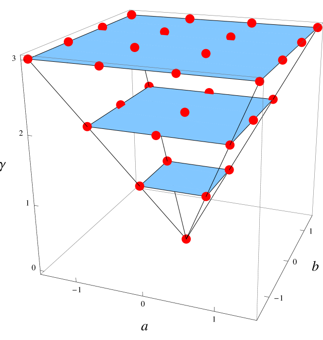
Figure 1: Degeneracy levels.

4 Another approach to the quantum case

Another equivalent way in order to find the SGA for the free particle in $S^{3}$ comes naturally by considering the canonical quantization of the Dirac brackets in (6). In this context, the canonical variables in (6) become densely defined Hermitian operators on $L^{2}(S^{3})$ and the Dirac brackets are transformed into commutators multiplied by $i$ whenever necessary for Hermiticity reasons. To simplify the notation, a quantum observable will be denoted by the capital letter that denotes the corresponding classical observable, so that the quantum Hermitian operators corresponding to $x_{i}$, $p_{i}$ will be designed by $X_{i},P_{i}$, respectively. They fulfill the commutation relations, which result from the canonical quantization of the above Dirac deformed Poisson brackets obtained by replacing the brackets $\{a,b\}=c$ by the commutators $[A,B]=-i\,C$ (where $A,B,C$ denote the quantum operators of the classical analogs $a,b,c$). In this case (6) becomes:

$$[X_{j},X_{k}]=0\,,\quad[P_{j},X_{k}]=-i(\delta_{jk}-X_{j}X_{k})\,,\quad[P_{j},P_{k}]=-iJ_{jk}\,.$$ (103)

The operators $J_{jk}$ keep the same expression as in the classical case taking care of the ordering,

$$J_{jk}=X_{j}P_{k}-X_{k}P_{j}\,.$$ (104)

From (104), we see that these operators are also Hermitian and $J_{jk}=-J_{kj}$. The above commutators imply that the operators $J_{jk}$ close indeed the Lie algebra $\mathfrak{so}(4)$ and that ${\bf X}$ and ${\bf P}$ are four vectors under the $J_{jk}$ generators, i.e., relations (10)-(12) are implemented through commutators at the quantum level.

In the classical discussion, we have established the need of a constraint (3) and a gauge fixing condition (5) for the classical variables, and the same has to be done in the quantum frame for the corresponding quantum operators. Here, the gauge condition is chosen to be

$${\bf X}^{2}=1\,,$$ (105)

which is consistent with the fact that the configuration space is $S^{3}$. The classical constrain $\bf{xp}=0$ should be here expressed in terms of the symmetrized operator $(\bf{XP}+\bf{PX})/2$. In this respect, first note that that the generators $\bf{XP}$ and $\bf{PX}$ commute with any position $X_{i}$ or momentum $P_{j}$ operators. Then, from (103) and (104), we obtain the following relations:

$$\bf{XP}=\bf{PX}+3i$$ (106)

$$J_{ik}X_{k}=-P_{i}+X_{i}(\bf{PX})$$ (107)

$$X_{k}J_{ik}=-P_{i}+X_{i}(\bf{XP})\,.$$ (108)

Summing (107) and (108), we have

$$\frac{1}{2}\,(J_{ik}X_{k}+X_{k}J_{ik})=-P_{i}+\frac{1}{2}\,X_{i}(\bf{PX}+\bf{XP})\,.$$ (109)

We must be aware that the initial algebra (103) generated by $\{\bf{X},\bf{P}\}$ remains invariant if we replace the ‘momentum’ operators by another set $\bf{P}\to\bf{P}+\alpha\bf{X}$, $\alpha$ being a number or a central element. We can use this freedom to get simpler expressions. Thus, we define a new momentum in the form

$$\widetilde{\bf{P}}:=\bf{P}-\frac{1}{2}\,X_{i}(\bf{PX}+\bf{XP})\,.$$ (110)

We can interpret $\widetilde{\bf{P}}$ as the quantum analog of the projection of the vector $\bf{P}$ on the tangent plane to the point of the sphere characterized by the vector $\bf{X}$. Thus, $\widetilde{\bf{P}}$ should be the proper definition for the quantum momentum operator corresponding to the motion on $S^{3}$. Since $\widetilde{J_{ik}}:=X_{i}\widetilde{P_{k}}-X_{k}\widetilde{P_{i}}=X_{i}P_{k}-P_{k}X_{i}=J_{ik}$, the set $\{\bf{X},\widetilde{\bf{P}}\}$ has the same formal commutation relations as (103). This leads to the following simplified relations:

$$\bf{X}\widetilde{\bf{P}}+\widetilde{\bf{P}}\bf{X}=0\,,$$ (111)

$$\bf{X}\widetilde{\bf{P}}=-\widetilde{\bf{P}}\bf{X}=\frac{3i}{2}\,,$$ (112)

$$\frac{1}{2}\,(J_{ik}X_{k}+X_{k}J_{ik})=-\widetilde{P}_{i}\,.$$ (113)

Relations (105), (111) and (113) are the quantum versions of the classical formulas (5), (3) and (23), respectively. In the sequel, we shall always use $\widetilde{P}_{i}$ instead of $P_{i}$, although henceforth we shall remove the tilde for convenience.

As a remark, let us say that we can provide a realization of the operators $X_{i},P_{j}$, satisfying the previous relations, in terms of the canonical operators in $\mathbb{R}^{4}$ (which are uniquely defined up to a unitary equivalence). This realization is given by

$$\begin{array}[]{l}X_{i}({\boldsymbol{\Xi}},{\boldsymbol{\Pi}}):=\frac{\Xi_{i}}{\Xi}\,,\\[8.61108pt] P_{i}({\boldsymbol{\Xi}},{\boldsymbol{\Pi}}):=\frac{1}{2}(\Xi\Pi_{i}+\Pi_{i}\Xi)-\left(({\boldsymbol{\Pi}}{\boldsymbol{\Xi}}+{\boldsymbol{\Xi}}{\boldsymbol{\Pi}})\frac{\Xi_{i}}{4\,\Xi^{2}}+\frac{\Xi_{i}}{4\,\Xi^{2}}({\boldsymbol{\Pi}}{\boldsymbol{\Xi}}+{\boldsymbol{\Xi}}{\boldsymbol{\Pi}})\right)\,,\end{array}$$ (114)

where ${\boldsymbol{\Pi}}$ and ${\boldsymbol{\Xi}}$ satisfy the canonical commutators

$$[\Xi_{j},\Pi_{k}]=i\,\delta_{ij},\quad[\Xi_{j},\Xi_{k}]=[\Pi_{j},\Pi_{k}]=0$$ (115)

and $\Xi=\sqrt{\sum_{k}(\Xi_{k})^{2}}$. This is the quantum analog of the classical expressions given in (8).

Likewise the classical case, one of the $\mathfrak{so}(4)$ Casimirs plays the role of the Hamiltonian operator

$$H=\frac{1}{2}\;J_{jk}J_{jk}={\bf P}^{2}-(\bf{PX})(\bf{XP})={\bf P}^{2}-9/4\,,$$ (116)

where we have taken into account the restrictions on $\bf{X}$ and $\bf{P}$ of (105), (111) and (112). In the $\mathfrak{so}(4)$ realization given by (103) and (104), the second Casimir vanishes:

$$C_{2}=\frac{1}{2}\epsilon^{ijkl}J_{ij}J_{kl}=0\,.$$ (117)

4.1 The quantum Spectrum Generating Algebra

In the context of the point of view of the present section, in order to construct the Spectrum Generating Algebra (SGA) for the free particle $S^{3}$ we will consider the algebra generated by all the operators $\{X_{i},P_{j},J_{kl},H\}$, including the Hamiltonian.

We must compute the commutation of $X_{i}$ and $P_{j}$ with $H$. From (103)-(104), after some straightforward computations, we get

$$[H,X_{i}]=-i\,2P_{i}$$ (118)

and

$$[H,P_{i}]=-i\bf g((2H+3/2)X_{i}-2P_{i}\bf g)\,.$$ (119)

The commutators (118) and (119) give a linear action of $H$ on the elements having the form $\alpha(H)X_{i}+\beta(H)P_{i}$, where the coefficients $\alpha,\beta$ may depend on $H$. We can diagonalize this action as an eigenvalue problem:

$$[H,V_{i}^{\pm}]=\lambda^{\pm}(H)V_{i}^{\pm}\,.$$ (120)

The solution of this eigenvalue equation is straightforward. The respective eigenvalues and eigenvectors are

$$\lambda^{\pm}(H)=-1\pm 2h\,,\qquad{\rm with}\qquad h:=\sqrt{H+1}\,,$$ (121)

$$V_{i}^{\pm}=-i(\pm h+1/2)X_{i}-P_{i}\,,$$ (122)

where we must taking care of the order of $h$ and $X_{i}$. The eigenvectors $V_{i}^{\pm}$ are defined up to global factors that may depend on $h$, this freedom will be used later.

Let us go back to the discussion on Section 3.1. There, we have shown that the operator $h$, as defined in (121) has a purely discrete spectrum coinciding with the set of natural numbers. We can summarize this in the following formulas

$$H=h^{2}-1,\quad{\rm Spec}(h)=1,2,\dots\,.$$ (123)

Now, let us rewrite (120) as

$$(H-\lambda^{\pm})V_{i}^{\pm}=V_{i}^{\pm}H\,.$$ (124)

Taking into account (123) and replacing $\lambda^{\pm}$ into (124), we have

$$(h\mp 1)V_{i}^{\pm}=V_{i}^{\pm}h\,.$$ (125)

Therefore, $V_{i}^{\pm}$ act as lowering and raising operators for $h$, changing its eigenvalues in one unit.

Our next task is to express the initial (quadratic) algebra generated by $\{X_{i},P_{j},H,J_{ik}\}$ in terms of the most appropriate basis $\{V_{i}^{\pm},h,J_{ik}\}$. In order to calculate the commutation of $V_{i}^{\pm}$ among themselves, we must express $X_{i}$ and $P_{i}$ in terms of these eigenvectors (or eigenoperators) $V_{i}^{\pm}$:

$$X_{i}=\frac{i}{2h}\;\big{(}V_{i}^{+}-V_{i}^{-}\big{)}\,,\qquad P_{i}=-\frac{1}{2h}\big{(}V_{i}^{+}(h+1/2)-(h+1/2)V_{i}^{-}\big{)}\,.$$ (126)

Then, making use of the commutators of $h$ with $V_{i}^{\pm}$ (125) we can easily compute the commutators of $X_{i}$ and $P_{i}$ with a general function $F(h)$ of $h$. Therefore, we obtain without difficulty that

$$X_{i}\,F(h)=\frac{1}{2h}\left\{F(h{-}1)(h+1/2)-F(h{+}1)(-h+1/2)\right\}X_{i}$$ (127)

$$\hskip 28.45274pt-\frac{i}{2h}\,\left\{F(h{-}1)-F(h{+}1)\right\}P_{i}\,,$$

and

$$P_{i}\,F(h)=\frac{i}{2h}\,\left\{F(h{-}1)(h^{2}-1/4)-F(h{+}1)(h^{2}-1/4)\right\}X_{i}$$

$$\hskip 28.45274pt+\frac{1}{2h}\,\left\{F(h{-}1)(h-1/2)+F(h{+}1)(h+1/2)\right\}P_{i}\,.$$ (128)

We have already computed the commutators of $h$ with $V_{i}^{\pm}$ and, since the symmetry algebra of $H$ is spanned by $J_{ij}$, we have $[h,J_{ik}]=0$. Thus, the only commutators that remain to be found are those involving the eigenoperators $V_{i}^{\pm}$. After some lengthy but straightforward calculations, we find

$$[V_{i}^{-},V_{j}^{+}]=2h\delta_{ij}+2iJ_{ij}\,,\quad[V_{i}^{+},V_{j}^{+}]=[V_{i}^{-},V_{j}^{-}]=0\,.$$ (129)

At this point, we should remark that the eigenoperators $V_{i}^{\pm}$ given in (120) are defined up to a factor that can depend on $h$, so that we may replace $V_{i}^{\pm}$ by expressions like $f(h)V_{i}^{\pm}g(h)$. This fact can be used, for instance, to construct a new pairs of eigenoperators each one adjoint of the other. Then, since

$$(V_{i}^{+})^{\dagger}=\frac{h+1}{h}\,V_{i}^{-}\,,$$ (130)

we can define

$$A_{i}^{\pm}:=\frac{1}{\sqrt{h}}\,V_{i}^{\pm}\,\sqrt{h}\,,\qquad i=1,2,3,4\,,$$ (131)

so that

$$(A_{i}^{+})^{\dagger}=A_{i}^{-}\,.$$ (132)

Then, we can restate the relevant relations involving $V_{i}^{\pm}$ in terms of $A_{i}^{\pm}$. We begin with (125):

$$[h,A^{\pm}_{i}]=\pm A^{\pm}\,.$$ (133)

Next, we can express $X_{i}$ and $P_{i}$ as in (126) in the following form:

$$X_{i}=\frac{i}{2}\frac{1}{\sqrt{h}}\;(A_{i}^{+}-A_{i}^{-})\frac{1}{\sqrt{h}}\,,\qquad P_{i}=-\frac{1}{2}\frac{1}{\sqrt{h}}\;\big{(}A_{i}^{+}(h+1/2)+(h+1/2)A_{i}^{-}\big{)}\frac{1}{\sqrt{h}}\,.$$ (134)

The last formula in (134) may also be written as

$$P_{i}=-\frac{1}{2}\,\frac{f(h)}{\sqrt{2h}}\;(A_{i}^{+}+A_{i}^{-})\frac{f(h)}{\sqrt{2h}}\,,$$ (135)

where the function $\phi$ is characterized by

$$2h+1=f(h)f(h+1)\,.$$ (136)

Equation (136) is identical to (85) and therefore it has the same solution (86). Finally, commutation relations (129) are preserved:

$$[A_{i}^{-},A_{i}^{+}]=2h\delta_{ij}+2iJ_{ij}\,,\quad[A_{i}^{+},A_{j}^{+}]=[A_{i}^{-},A_{j}^{-}]=0\,.$$ (137)

Now, we are in position to obtain the generators of the $\mathfrak{so}(4,2)$ Lie algebra from the above ingredients. Then, we can define the following new operators

$$L_{i}:=\frac{1}{2i}\,(A_{i}^{-}-A_{i}^{+})\,,\quad{\rm and}\quad{K}_{i}:=\frac{1}{2}\,(A_{i}^{-}+A_{i}^{+})\,.$$ (138)

Using the commutation relations obtained before in this Section, it is easy to show that set of the operators

$$\{J_{ij},h,L_{i},K_{i}\}$$ (139)

form a basis for $\mathfrak{so}(4,2)$. In fact, if we make the following identifications

$$J_{ij}\equiv M_{ij}\,,\quad{K}_{i}\equiv M_{5i}\,,\quad L_{i}\equiv M_{6i}\,,\quad h\equiv M_{56}\,,\quad i,j=1,\dots,4\,,$$ (140)

then, $M_{\alpha\beta}$, $\alpha,\beta=1,\dots,6$ will satisfy the commutation relations (37). The vector character of the components $L_{i}$ and $K_{i}$ or the scalar behaviour of $h$ under $\mathfrak{so}(4)$ are satisfied from its very definition in terms of the vectors $X_{i}$, $P_{i}$ and the scalar $H$. Notice that, according to (134) and (135), we have

$$K_{i}=-\frac{\sqrt{2h}}{f(h)}\,P_{i}\,\frac{\sqrt{2h}}{f(h)},\qquad L_{i}=\sqrt{h}\,X_{i}\sqrt{h}\,.$$ (141)

We can avoid the use of the $f(h)$ function in in the relation between $P_{i}$ and $K_{i}$ as follows. For instance, take the second equation in (134) and re-express it in the form

$$P_{i}=-\frac{1}{\sqrt{h}}\,\frac{1}{4}\,[h(A_{i}^{-}+A_{i}^{+})+(A_{i}^{-}+A_{i}^{+})h]\,\frac{1}{\sqrt{h}}=-\frac{1}{2}\,\frac{1}{\sqrt{h}}\,(h{K}_{i}+{K}_{i}h)\,\frac{1}{\sqrt{h}}\,.$$ (142)

These relations, together with $h=\sqrt{H-1}$ (121), constitute the quantum analogue of the classical ones given by (24).

We have already mentioned in (123) that the spectrum of the operator $h$ is the set of natural nubers $n=1,2,3,\dots$ while the spectrum of the Hamiltonian $H$ is given by $n^{2}-1$. These energy levels can be connected by a ladder representation, which follows from the nature of the operators $A_{i}^{\pm}$ and that is identical to the representation given in section 3.3. This shows that $\mathfrak{so}(4,2)$ is the SGA for the quantum particle in $S^{3}$.

4.2 The restrictive relations.

In Section 3, we have started directly with the quantization of the algebra $\mathfrak{so}(4,2)$, including the operators $A_{i}^{\pm}$. Then, some naturally chosen restrictive conditions allowed us to define the generators $X_{i}$ of the homogeneous space (and their corresponding momenta $P_{i}$) satisfying commutation relations (103). Now, we will finish by showing that the above construction yields naturally to the restrictive relations as given by (59).

In the previous subsection we have shown that the quantum SGA was a Lie algebra obtained from the quadratic algebra generated by $\{X_{i},P_{j},J_{ij},H\}$ after a (generalized) change of basis. As the starting generators were not independent so there must be certain relations involving the Lie algebra generators that will turn into the restrictive conditions. In fact, in order to make all the computations in the above subsection we have made use of two relations: (i) the expression of $J_{ij}$ in terms of $X_{i},P_{j}$, as given in (104) that is equivalent to the vanishing of the second Casimir (117) of $\mathfrak{so}(4)$, and (ii) the choice of $P_{i}$ given in terms of $J_{ij}$ and $X_{j}$ in (113).

Let us start with the relation (ii) where we substitute $P_{i}$ in terms of $K_{i}$ by means of (142), $X_{j}$ in terms of $L_{j}$ as shown in (141), to get

$$J_{ik}\,\frac{1}{\sqrt{h}}\,L_{k}\,\frac{1}{\sqrt{h}}+\frac{1}{\sqrt{h}}\,L_{k}\,\frac{1}{\sqrt{h}}\,J_{ik}=\frac{1}{\sqrt{h}}\,(h{K}_{i}+{K}_{i}h)\,\frac{1}{\sqrt{h}}\,.$$ (143)

Since $h$ and $J_{ik}$ commute, equation (143) becomes:

$$J_{ik}L_{k}+L_{k}J_{ik}-h{K}_{i}-{K}_{i}h=0\,.$$ (144)

Now taking into account the identification with the generators $M_{\alpha\beta}$ of $\mathfrak{so}(4,2)$, this equation is just $\widetilde{T}_{6i}=0$, thus obtaining the first restrictive relation. The remaining relations are obtained by commuting (144) with other operators. For instance, let us commute (144) with $h$, then we find a second restrictive relation:

$$J_{ik}{K}_{k}+{K}_{k}J_{ik}+hL_{i}+L_{i}h=0\qquad{\rm or}\qquad\widetilde{T}_{5i}=0\,.$$ (145)

The next one can be obtained by commuting $L_{i}$ with (144), summing over $i$ and taking into account that

$$[L_{i},J_{ik}]=-3iL_{k}\,,$$ (146)

then, we arrive to the relation:

$${\bf K}^{2}-3{\bf L}^{2}+2h^{2}+2=0\,.$$ (147)

Now, we commute (145) with $K_{i}$ and sum over $i$ to find:

$${\bf L}^{2}-3{\bf K}^{2}+2h^{2}+2=0\,.$$ (148)

Relations (147) and (148) together yield

$${\bf K}^{2}-h^{2}-1=0\qquad{\rm or}\qquad\widetilde{T}_{55}=0\,,$$ (149)

$${\bf L}^{2}-h^{2}-1=0\qquad{\rm or}\qquad\widetilde{T}_{66}=0\,.$$ (150)

Next, we commute $L_{i}$ with (145) and sum over $i$. We obtain:

$${\bf K}\cdot{\bf L}+{\bf L}\cdot{\bf K}=0\qquad{\rm or}\qquad\widetilde{T}_{56}=0\,.$$ (151)

The last of the relations $\widetilde{T}_{ab}=0$ follows by commuting $L_{j}$ with (144). It gives:

$$(L_{i}L_{j}+L_{j}L_{i})+(K_{i}K_{j}+K_{j}K_{i})-(J_{ik}J_{jk}+J_{jk}J_{ik})-2\delta_{ij}=0\,,$$ (152)

or $\widetilde{T}_{ij}=0$. Note that the constant $c$ in (49)-(54) appears naturally as $c=2$.

The other restrictive relations in (59), $R^{ab}=0$, can be obtained as follows: The former, $R^{56}=0$ is just the expression (117) stating that the second Casimir vanishes in the chosen representation. Then, commute (117) with $L_{j}$ and $K_{i}$ to obtain $R^{6i}=0$ and $R^{5i}=0$ respectively. Then, using the explicit relation for $R^{5i}$ given in (56) and commuting $R^{5i}=0$ with $L_{i}$, one finally gets the last relation $R^{ij}=0$. Explicit forms of $R^{ab}$ are given in (55)-(58). With the derivation of the restrictive relations, we conclude the present section.

5 Concluding remarks.

In this paper, we have constructed the Spectrum Generating Algebra (SGA) for the three dimensional sphere $S^{3}$ in both classical and quantum cases. Both situations provide a nontrivial problem, particularly in the quantum case.

In the classical case, we have obtained specific SGA generators leading to time dependent constants of motion fixing the motion. In the quantum case, we can study the SGA for $S^{3}$ from two points of view. In the former, we start with a quantized version of the algebra, postulate natural restrictive relations that fixes the representation and then, obtaining a ladder representation that connect the whole set of eigenvectors of the free Hamiltonian for $S^{3}$, supporting the Hilbert space of an IUR of the SGA algebra. Finally, we define the position and momentum operators for the homogeneous ambient space and fix their constraints and gauge conditions over $S^{3}$ and their commutation relations.

The second point of view is equivalent and makes the inverse path. We start with quantization of the position and momentum operators by transforming their Dirac brackets into commutators following the usual recipe established by usual canonical quantization. These operators determine a representation of the algebra ${\mathfrak{s}o}(4)$. Then, we construct ladder operators and determine that the SGA for our situation is ${\mathfrak{s}o}(4)$. Finally, the restrictive relations postulated in the previous method are obtained as a consequence of our hypothesis.

This research as interest by itself, although we expect this work to serve as a preparation for the construction of the SGA of non trivial potentials in $S^{3}$ as well as in a spaces with negative curvature $H^{3}$, under the same optics.

References

References

• [1] A.O. Barut, A. Bohm, Phys. Rev, 139, B1107 (1965).
• [2] Y. Dothan, M. Gell-Mann, Y. Ne’eman, Phys. Lett, 17, 148 (1965).
• [3] Y. Dothan, Phys. Rev. D 2, 2944 (1970).
• [4] E. SchrΓΆdinger, Proc. R.I.A. A 49, 9-16 (1940).
• [5] S. Kuru and J. Negro, Ann. Phys., 323, 413 (2008).
• [6] S. Kuru and J. Negro, Ann. Phys., 324, 2548 (2009).
• [7] C. Quesne, J. Phys. A, 21, 4487 (1988).
• [8] A. Bohm, Y. Neeman, Dynamical Groups and Spectrum Generating Algebras in Dynamical Groups and Spectrum Generating Algebras, Edited by A. Barut, A. Bohm and Y. Neeman, (World Scientific, Singapur 1988).
• [9] G.P. Pronko, Theoretical and Mathematical Physics, 155, 780 (2008).
• [10] P.A.M. Dirac, Lectures on Quantum Mechanics, (Belfer Graduate School of Science Monographs Series Number 2, 1964).
• [11] E.C.G. Sudarshan, N. Mukunda, Classical Dynamics: A Modern Perspective (Wiley, New York, Toronto, 1974).
• [12] A. O. Barut, R. Raczka, Theory of Group Representations and Applications (World Scientific, Singapur, 1986).