A newly discovered DLA and associated Ly$\alpha$ emission in the spectra of the gravitationally lensed quasar UM 673A,B

Abstract

The sightline to the brighter member of the gravitationally lensed quasar pair UM 673A,B intersects a damped Ly$\alpha$ system (DLA) at $z=1.62650$ which, because of its low redshift, has not been recognised before. Our high quality echelle spectra of the pair, obtained with HIRES on the Keck i telescope, show a drop in neutral hydrogen column density $N$(H i) by a factor of at least 400 between UM 673A and B, indicating that the DLA’s extent in this direction is much less than the $2.7\,h_{70}^{-1}$ kpc separation between the two sightlines at $z=1.62650$. By reassessing this new case together with published data on other quasar pairs, we conclude that the typical size (radius) of DLAs at these redshifts is $R\simeq(5\pm 3)\,h_{70}^{-1}$ kpc, smaller than previously realised. Highly ionized gas associated with the DLA is more extended, as we find only small differences in the C iv absorption profiles between the two sightlines.

Coincident with UM 673B, we detect a weak and narrow Ly$\alpha$ emission line which we attribute to star formation activity at a rate ${\rm SFR}\lower 2.15277pt\hbox{$\;\buildrel>\over{\sim}\;$}0.2$ M_⊙ yr^-1. The DLA in UM 673A is metal-poor, with an overall metallicity $Z_{\rm DLA}\simeq 1/30Z_{\odot}$, and has a very low internal velocity dispersion. It exhibits some apparent peculiarities in its detailed chemical composition, with the elements Ti, Ni, and Zn being deficient relative to Fe by factors of 2–3. The [Zn/Fe] ratio is lower than those measured in any other DLA or Galactic halo star, presumably reflecting somewhat unusual previous enrichment by stellar nucleosynthesis. We discuss the implications of these results for the nature of the galaxy hosting the DLA.

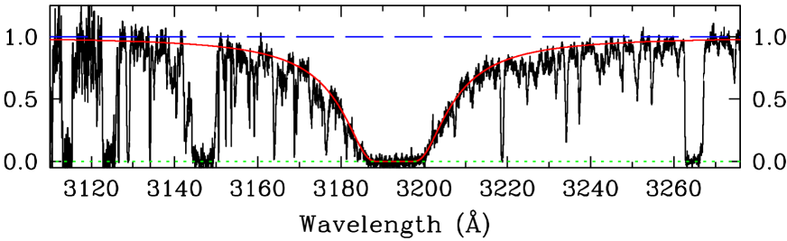
Figure 1: Portion of the HIRES spectrum of UM 673A (black histogram) encompassing the damped Ly$\alpha$ line at $z_{\rm abs}=1.626498$. The red continuous line shows the theoretical Voigt profile for a neutral hydrogen column density $\log[N({\rm H}\,\textsc{i})/{\rm cm}^{-2}]=20.7$. The normalised continuum and zero-level are shown by the blue dashed and green dotted lines respectively. The $y$-axis scale is residual intensity.

1 Introduction

UM 673 (Q0142$-$100) was first identified as a gravitationally lensed quasar (QSO) at $z_{\rm em}=2.719$ by Surdej et al. (1987) who showed it to be lensed by a $z=0.49$ galaxy into two images, UM 673A and UM 673B, separated by 2.2 arcsec and with magnitudes $m_{\rm R}=16.9$ and 19.1 respectively. This pair was later examined in detail by Smette et al. (1992) in their study of intergalactic Ly$\alpha$ forest absorbers. By considering the number of absorption lines in common (and not in common) between the two closely spaced sightlines, these authors were able to place interesting limits on the typical sizes of Ly$\alpha$ clouds, following on from analogous analyses by Sargent et al. (1982) and Foltz et al. (1984).

Since these early papers, there have been many investigations of the Ly$\alpha$ forest in the spectra of gravitationally lensed QSOs. However, very little is still known about the size and geometry of the neutral gas reservoirs that give rise to DLAs with hydrogen column densities $N(\textrm{H}\,\textsc{i})$ $\geq\,2\times 10^{20}\,{\rm cm}^{-2}$, since these are much rarer absorption systems and thus unlikely to be found in front of gravitationally lensed QSOs which are themselves unusual alignments. A recent study by Monier et al. (2009) of the quadruply lensed Cloverleaf QSO (H 1413+117) with the Hubble Space Telescope uncovered three new DLAs or sub-DLAs at $z\sim 1.5$, none of which are common to all four components. When considered together with analogous observations of four other DLAs from the literature, these data led Monier et al. (2009) to conclude that absorbers at $z\sim 1.5$ with $N(\textrm{H}\,\textsc{i})$ $=(6-13)\times 10^{20}\,{\rm cm}^{-2}$ have typical scale-lengths ${\rm S}_{\rm DLA}=(6-12)\,h_{70}^{-1}\,{\rm kpc}$ (where $h_{70}$ is the Hubble constant in units of 70 km s^-1 Mpc^-1).

Apparently at odds with this conclusion is the finding by Ellison et al. (2007) of coincident damped Lyman alpha absorption on 100 kpc-scale towards the binary QSO SDSS 1116+4118A,B. As these dimensions far exceed those expected for a single galaxy, Ellison et al. (2007) favour an explanation in terms of a group of two or more galaxies intersected along these lines of sight.

In this paper we report the discovery of a previously unrecognised DLA, at $z_{\rm abs}=1.62650$, in the spectrum of UM 673A from high resolution and high signal-to-noise ratio (S/N) spectroscopy with the HIRES instrument on the Keck i telescope. In line with the compilation of similar measurements by Monier et al. (2009), no DLA is seen in front of UM 673B, even though at the redshift of the DLA the two sightlines are separated by less than 3 kpc.

We do, however, find a weak Ly$\alpha$ emission line in the spectrum of UM 673B at the same redshift as the DLA. There have been only a few reported cases of Ly$\alpha$ emission associated with a DLA since the first such detection by Hunstead et al. (1990), as summarised in the review of DLA properties by Wolfe et al. (2005) with more recent updates by Kulkarni et al. (2006) and Christensen et al. (2007). Any new examples are of interest in view of the apparent puzzle presented by the lack of obvious star formation associated with gas-rich DLAs (Wolfe & Chen, 2006), and the recent claim that a newly discovered population of faint line emitters represents the long-sought host galaxies of DLAs (Rauch et al., 2008).

Finally, the newly discovered DLA in UM 673A is metal-poor, with metallicity $Z\sim 1/30Z_{\odot}$. Such chemically unevolved DLAs are important, in that they can provide clues to early episodes of metal enrichment in the Universe, complementing efforts being directed to analogous studies of metal-poor stars in the Milky Way and nearby dwarf galaxies (see, for example, Pettini, 2006). In the present case, we measure the relative abundances of nine different elements, from N to Zn, and uncover some chemical peculiarities which have not been noted before.

The paper is organised as follows. In Section 2, we briefly describe the observations of UM 673A,B and the reduction of the HIRES spectra. In the subsequent analysis, we first focus on the H i gas in front of the UM 673 pair (Section 3), and consider the data presented here together with the compilation by Monier et al. (2009) of other DLAs in gravitationally lensed QSOs to refine those authors’ estimate of the characteristic size of damped systems (Section 4). We next turn to the Ly$\alpha$ emission detected in the spectrum of UM 673B at the same redshift as the DLA in UM 673A (Section 5), and use it to obtain an estimate of the star formation rate in the galaxy associated with the DLA. Section 6 deals with the chemical composition of the DLA, comparing it to that of DLAs and Galactic halo stars of similar overall metallicity. We summarise our findings and draw some conclusions in Section 7. Throughout the paper, we adopt a ‘737’ cosmology, with $H_{0}=70\,{\rm km\,s}^{-1}\,{\rm Mpc}^{-1}$, $\Omega_{\rm M}=0.3$ and $\Omega_{\Lambda}=0.7$.

2 Observations and Data Reduction

We observed UM 673A and UM 673B on the nights of 2005 October 9 and 10, and again three years later on the nights of 2008 September 24 and 25, as part of a large-scale imaging and spectroscopic survey of galaxies in the fields of bright QSOs, aimed primarily at studying the outflows of interstellar gas from star-forming galaxies at redshifts $z=2$–3 (Adelberger et al., 2005; Steidel et al., 2010). HIRES (Vogt et al., 1994) was configured to cover the wavelength range 3100–6100 Å (with small gaps near 4000 Å and 5000 Å due to gaps between the three CCD chips on the detector) using the ultraviolet (UV) cross-disperser and collimator.

In order to avoid cross-contamination between the two images and to minimize slit losses due to atmospheric dispersion, UM 673 A and B were observed separately, with the HIRES slit maintained at the parallactic angle by its image rotator. For UM 673 A we used a 1.15 arcsec-wide entrance slit, which results in a resolution $R\equiv\lambda/\Delta\lambda=36\,000$, corresponding to a velocity full width at half maximum ${\rm FWHM}=8.3$ km s^-1, sampled with $\sim 3$ pixels. The total integration time was $9400\,{\rm s}$, divided into five exposures; the QSO was stepped along the slit between each exposure. For the fainter UM 673 B, we employed the narrower 0.86 arcsec slit (so as to exclude more effectively light from the brighter image) which results in $R=48\,000$ and ${\rm FWHM}=6.2$ km s^-1 sampled with $\sim 2$ detector pixels. The total exposure time was $28\,200\,{\rm s}$, again divided into a number of separate exposures, typically 2700 s long. The seeing was $\leq 1$ arcsec FWHM throughout the observations.

To these data we added another set of observations of UM 673A,B, which we retrieved from the Keck Observatory data archive, obtained in 1996 with the original HIRES red-sensitive detector and red-optimized cross-disperser. While these earlier data do not contribute much at blue and ultraviolet wavelengths, with their long exposure times (18 000 s and 27 000 s for UM 673A and B respectively) they do improve the S/N ratio of our final co-added spectrum at red wavelengths.

The two-dimensional HIRES spectra were processed with the makee data reduction pipeline developed by Tom Barlow which includes the usual steps of flat-fielding, order tracing, background subtraction, 1-D extraction and merging of the echelle orders. A wavelength reference was provided by the spectrum of the internal Th-Ar hollow cathode lamp and the co-added, 1-D spectra were mapped onto a vacuum heliocentric wavelength scale. In a final step, the spectra were normalised by dividing out the QSO continuum and emission lines. The rms deviations of the data from the continuum in regions free from absorption lines provide an empirical measure of the signal-to-noise ratio. For UM 673A, our data have ${\rm S/N}>35$ per 2.7 km s^-1 ($\approx 0.04$ Å) bin from $\sim 4000$ Å to $\sim 6000$ Å; the S/N is highest near 5000 Å (${\rm S/N}\simeq 70$) and is still moderately high (${\rm S/N}\simeq 24$) at 3200 Å, near the redshifted wavelength of the damped Ly$\alpha$ line. The corresponding values for UM 673B are ${\rm S/N}\lower 2.15277pt\hbox{$\;\buildrel>\over{\sim}\;$}15$ (4000–6000 Å) and ${\rm S/N}\simeq 8$ at 3200 Å.

3 H i Absorption towards UM 673A,B

3.1 The DLA towards UM 673A

Our HIRES spectra extend to shorter wavelengths than most previous observations of this famous QSO pair, which probably explains why the damped Ly$\alpha$ system in front of UM 673A (see Fig. 1) has gone unnoticed until now. Associated with the DLA are a multitude of metal absorption lines of elements from C to Zn. These lines are analysed in detail in Section 6; for the present purpose suffice it to say that they are narrow, with ${\rm FWHM}\lower 2.15277pt\hbox{$\;\buildrel<\over{\sim}\;$}25$ km s^-1, and have maximum optical depth at $z_{\rm abs}=1.626498$. Adopting the same redshift for the damped Ly$\alpha$ line (which is too broad to allow such an accurate determination of $z_{\rm abs}$), we find $\log[N({\rm H}\,\textsc{i})/{\rm cm}^{-2}]=20.7\pm 0.1$ by fitting theoretical Voigt profiles to the wings of the line (and interpolating across narrower absorption features—see Fig. 1).

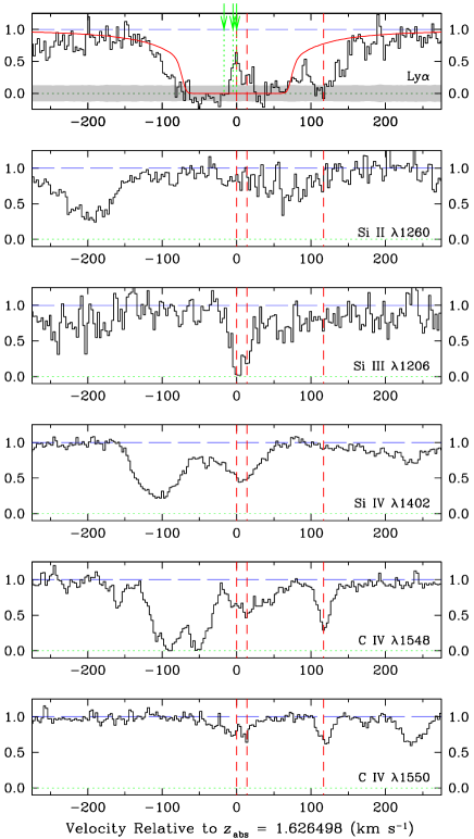
Figure 2: A selection of absorption lines in UM 673B near the redshift of the DLA at $z_{\rm abs}=1.626498$ in front of UM 673A; in all panels the $y$-axis is residual intensity. The three green arrows in the top panel indicate the velocities of the three components of the low-ionization metal lines in the DLA (see Section 6), while the three long-dash red lines through all the panels mark the velocities of absorption (and emission) components in UM 673B. In the top panel, the red continuous line is the theoretical Ly$\alpha$ absorption profile for the upper limit we deduce to the column density of neutral hydrogen in UM 673B, $\log[$$N(\textrm{H}\,\textsc{i})$$/{\rm cm}^{-2}]=18.1$. The grey shaded area shows the $\pm 1\sigma$ error spectrum. Note the detection of Ly$\alpha$ emission in the core of the strong absorption line, at the same redshift as the DLA in UM 673A. The emission profile also aligns well with the high ionization absorption lines in UM 673B reproduced in the lower four panels.

3.2 The Lyman limit system in UM 673B

We also find absorption near $z_{\rm abs}=1.626498$ in the spectrum of UM 673B, but with much reduced column densities of neutral gas. The top panel of Fig. 2 shows the wavelength region around the Ly$\alpha$ line which is broad and saturated, but not damped. Under these circumstances, it is well known that the column density is unconstrained within orders of magnitude, unless higher order Lyman lines are available—this is the reason why the H i column density distribution is so poorly sampled in the interval $\log[$$N(\textrm{H}\,\textsc{i})$$/{\rm cm}^{-2}]=17$–20 (e.g. Storrie-Lombardi & Wolfe, 2000; O’Meara et al., 2007).

However, since $N(\textrm{H}\,\textsc{i})$ and the velocity dispersion parameter $b$ (km s^-1) are degenerate in strongly saturated lines, we can still determine an upper limit to the column density by considering the smallest $b$-value, and corresponding highest value of $N(\textrm{H}\,\textsc{i})$, which provide an acceptable fit to the width and profile of the saturated Ly$\alpha$ line in UM 673B. To this end, we considered a series of pair values of $b$ and $N(\textrm{H}\,\textsc{i})$, fixing $N(\textrm{H}\,\textsc{i})$ and using vpfit to determine the value of $b$ for which the theoretical line profile shows the least disagreement with the data.

We started the iteration at $\log[$$N(\textrm{H}\,\textsc{i})$$/{\rm cm}^{-2}]=20.7$, as measured in UM 673A and which greatly overproduces the observed Ly$\alpha$ absorption in UM 673B for all values of $b$, and then decreased $\log$ $N(\textrm{H}\,\textsc{i})$ in steps of 0.1, until a plausible fit was arrived at for $\log[$$N(\textrm{H}\,\textsc{i})$$/{\rm cm}^{-2}]=18.1$ and $b=22\,{\rm km\,s}^{-1}$. The corresponding line profile, convolved with the instrumental resolution, is superimposed on the data in the top panel of Fig. 2. While the absorption in the line core is less than observed, presumably because of neighbouring Ly$\alpha$ absorption lines—one of which, at $\Delta v=+114$ km s^-1, is incidentally also seen as a redshifted component in C iv—higher column densities of $N(\textrm{H}\,\textsc{i})$ would overproduce the absorption in the line wings, relative to what is observed. We consider $\log[$$N(\textrm{H}\,\textsc{i})$$/{\rm cm}^{-2}]\leq 18.1$ to be an upper limit to the column density of neutral gas in UM 673B because equally good or even better fits could be obtained with lower values of $N(\textrm{H}\,\textsc{i})$ and higher values of $b$.

Thus, we are led to the conclusion that the column density of neutral hydrogen drops by a factor of at least 400 over a transverse distance of less than 3 kpc (Section 4). A comparable drop is deduced from consideration of metal absorption lines from ionization stages which are dominant in H i regions. For example, in Section 6, we deduce a column density $\log[N({\rm Si}\,\textsc{ii})/{\rm cm}^{-2}]=14.75\pm 0.03$ from the analysis of five Si ii transitions in UM 673A. The strongest of these, Si ii $\lambda 1260.4221$, is below the detection limit in UM 673B (see second panel from the top in Fig. 2). In the optically thin limit,

$$N=1.13\times 10^{20}\cdot\frac{W_{\lambda}}{\lambda^{2}f}~{}~{}{\rm cm}^{-2}$$ (1)

where $W_{\lambda}$ and $\lambda$ are respectively the rest frame equivalent width and wavelength (both in Å), and $f$ is the oscillator strength. From equation (1) we deduce $\log[N({\rm Si}\,\textsc{ii})/{\rm cm}^{-2}]\leq 12.2$ ($3\sigma$ limit) in UM 673B, a factor of $\geq 350$ lower than in UM 673A.

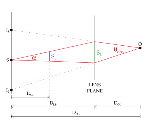
Figure 3: The geometry of a gravitational lens, as viewed by the observer at O, with source (S) being lensed into two images (${\rm I_{1}}$ and ${\rm I_{2}}$) of angular separation $\theta_{\rm obs}$, by a galaxy situated at the lens plane along the optical axis (dashed horizontal line). S₀ is the transverse distance between the two sightlines at the location of the galaxy producing the DLA.

4 Constraining the sizes of DLAs

Table 1: Derived e-folding scale lengths of DLAs, updated from Table 5 of Monier et al. (2009)

QSO	$z_{\rm em}$	$z_{\rm lens}$	$z_{\rm abs}$	Pair	$\theta_{\rm obs}$	$N({\rm H}\,\textsc{i})_{\rm max}$	$N({\rm H}\,\textsc{i})_{\rm min}$	${\rm S}_{0}^{\rm a}$	${\rm S}_{\rm DLA,\bar{e}}^{\rm b}$	${\rm S}_{\rm DLA,e}^{\rm c}$
					(arcsec)	($10^{20}\,{\rm cm}^{-2}$)	($10^{20}\,{\rm cm}^{-2}$)	($h_{70}^{-1}\,{\rm kpc}$)	($h_{70}^{-1}\,{\rm kpc}$)	($h_{70}^{-1}\,{\rm kpc}$)
H 1413+117	2.55	1.0	1.440	B-A	0.753	60	9.0	3.13	2.33	1.65
				B-D	0.967	60	0.25	4.02	2.55	0.733
				B-C	1.359	60	0.20	5.65	3.58	0.991
				A-D	1.118	9.0	0.25	4.64	3.02	1.29
				A-C	0.872	9.0	0.20	3.62	2.34	0.951
				D-C	0.893	0.25	0.20	3.71	11.7	16.6
H 1413+117			1.486	D-A	1.118	2.0	<0.05	4.32	<2.80	<1.17
				D-B	0.967	2.0	<0.1	3.73	<2.48	<1.25
				D-C	0.893	2.0	<0.05	3.45	<2.24	<0.935
H 1413+117			1.662	B-A	0.753	6.0	1.5	2.17	1.83	1.57
				B-C	1.359	6.0	0.6	3.91	2.75	1.70
				B-D	0.967	6.0	0.3	2.78	1.85	0.928
				A-C	0.872	1.5	0.6	2.51	2.64	2.74
				A-D	1.118	1.5	0.3	3.22	2.54	2.00
				C-D	0.893	0.6	0.3	2.57	3.25	3.71
HE 0512$-$3329	1.58	0.93	0.9313	A-B	0.644	3.09	2.95	5.05	70.4	109
Q 0957+561	1.4136	0.36	1.3911	A-B	6.2	1.9	0.8	0.278	0.303	0.321
UM 673	2.7313	0.493	1.6265	A-B	2.22	5.0	<0.013	2.71	<1.72	<0.455
HE 1104$-$1805	2.31	0.73	1.6616	A-B	3.0	6.3	<0.037	4.47	<2.84	<0.870

^a Transverse separation between the two sightlines at the redshift of the absorber.

^b $e$-folding scale length of DLA assuming a linear decline of $N$(H i)—see equation (7).

^c $e$-folding scale length of DLA assuming an exponential decline of $N$(H i)—see equation (9).

In this section we use the finding that the DLA in UM 673A is not present in the spectrum of UM 673B to reassess, together with existing data, the characteristic size of the H i clouds giving rise to damped Ly$\alpha$ systems.

We begin with a simple derivation of the transverse distance, similar to that presented by Smette et al. (1992). Referring to Fig. 3, the transverse distance between the two images at the lens plane is ${\rm S_{L}}=\theta_{\rm obs}\,{\rm D_{OL}}=\alpha\,{\rm D_{SL}}$, and the transverse distance between the two light paths at the redshift of the absorber is ${\rm S_{0}}=\alpha\,{\rm D_{SC}}$, where ${\rm D_{OL}}$, ${\rm D_{SL}}$, ${\rm D_{SC}}$ are the angular diameter distances from, respectively, the observer to the lens, the source to the lens, and the source to the absorbing cloud.

Thus, the transverse distance between the light paths at the redshift of the absorber can be written as

$${\rm S_{0}}=\frac{\theta_{\rm obs}\,{\rm D_{OL}\,D_{SC}}}{\rm D_{SL}}=\frac{\theta_{\rm obs}\,{\rm D_{OL}\,D_{CS}}}{\rm D_{LS}}\cdot\frac{(1+z_{\rm L})}{(1+z_{\rm C})}$$ (2)

where $z_{\rm L}$ and $z_{\rm C}$ are the redshifts of the lens and the DLA respectively. Recalling that the angular diameter distance between two objects at redshift $z_{2}$ and $z_{1}$, where $z_{2}\,>\,z_{1}$, is of the form (Hogg, 1999),

$${\rm D_{12}}=\frac{{\rm D}_{2}-{\rm D}_{1}}{1+z_{2}},$$ (3)

where

$${\rm D}_{i}=\frac{c}{H_{0}}\int_{0}^{z_{i}}\frac{dz}{\sqrt{\Omega_{\Lambda}+(1+z)^{3}\Omega_{\rm M}}}$$ (4)

is the comoving distance to redshift $z_{i}$, we can rewrite equation (2) as:

$${\rm S_{0}}=\frac{\theta_{\rm obs}\,{\rm D_{L}\,(D_{S}-D_{C})}}{(1+z_{\rm C}){\rm(D_{S}-D_{L})}}\,.$$ (5)

Thus, adopting $\theta_{\rm obs}=2.22$ arcsec, $z_{\rm L}=0.493$ (Surdej et al., 1988; Lehár et al., 2000), $z_{\rm S}=2.7434$ from our own unpublished near-infrared observations of the H$\beta$ emission line, and $z_{\rm C}=1.62650$ from the HIRES observations presented here, we find that the transverse (physical) distance between the two sightlines at the redshift of the DLA is ${\rm S_{0}}=2.7\,{\rm kpc}$ (in our ‘737’ cosmology).

We now add this new case to the list compiled by Monier et al. (2009) and reanalyse the entire sample in Table 1. Note that we have revised the values for the Cloverleaf (H 1413+117) from Table 5 of Monier et al. (2009) for two reasons. First, in calculating the transverse distances applicable to the two low redshift systems (at $z_{\rm abs}=1.440$ and 1.486) in the Cloverleaf, these authors assumed $z_{\rm L}=z_{\rm C}$ (E. Monier, private communication). Second, recent mid-infrared data have improved our understanding of this system (MacLeod et al., 2009). The positions and relative fluxes of the images can be well explained by a lensing galaxy at $z_{\rm L}\approx 1.0$ (Kneib, Alloin, & Pello, 1998), with an additional galaxy located $\Delta\alpha_{\rm G2}=-1.87$ arcsec, $\Delta\delta_{\rm G2}=4.14$ arcsec from the lens, coincident with a galaxy identified by Kneib et al. (1998) as object No. 14. The inclusion of this additional galaxy in the lensing model does not affect the astrometry (but does affect the relative fluxes of the QSO images); thus, we assumed a single lens geometry at $z=1.0$. We have excluded from the Monier et al. (2009) sample the binary QSO LBQS 1429$-$0053 because the linear scale probed by that pair, ${\rm S}_{0}=43.2\,h_{70}^{-1}$ kpc, is one order of magnitude larger than those of all the other (gravitationally lensed) pairs considered here. As argued by Ellison et al. (2007), such large scales are more likely to probe the clustering properties of DLAs rather than the typical sizes of their host galaxies. In any case, our conclusions below on the median size of DLAs are unaltered by the inclusion or omission of LBQS 1429$-$0053.

In order to determine the characteristic size of DLAs, ${\rm S_{DLA}}$, we adopt two simple models. In the first, ${\rm S_{DLA}}$ depends linearly on the H i column density, while in the second ${\rm S_{DLA}}$ depends linearly on the logarithm of $N(\textrm{H}\,\textsc{i})$. The latter is probably more realistic, as it corresponds to an exponential decline of $N(\textrm{H}\,\textsc{i})$, but we also consider the former for comparison with the analysis by Monier et al. (2009). Our analysis, however, differs from theirs in the following way. Monier et al. (2009) examined $N(\textrm{H}\,\textsc{i})$ as a function of the observed angular separation of two QSO images, $\theta_{\rm obs}$, whereas we considered $N(\textrm{H}\,\textsc{i})$ as a function of the physical (transverse) distance between the two sightlines at the redshift of the absorber. The approach taken by Monier et al. (2009) has the advantage of being independent of the choice of cosmological parameters, while ours is perhaps more physically motivated. We therefore have an equation of the form,

$${\rm S}={\rm S}_{0}\,\frac{N({\rm H}\,\textsc{i})_{\rm max}-N({\rm H}\,\textsc{i})}{N({\rm H}\,\textsc{i})_{\rm max}-N({\rm H}\,\textsc{i})_{\rm min}},$$ (6)

where $N({\rm H}\,\textsc{i})_{\rm max}$ is the higher column density observed between any two given sightlines, and $N({\rm H}\,\textsc{i})_{\rm min}$ is the lower column density of the two. In the first model, we follow Monier et al. (2009) and define the linear $e$-folding scale-length (${\rm S}_{\rm DLA,\bar{e}}$) to be the transverse distance over which $N(\textrm{H}\,\textsc{i})$_max decreases by a factor of $e=2.718$ (i.e. $N({\rm H}\,\textsc{i})=N({\rm H}\,\textsc{i})_{\rm max}/2.718$),

$${\rm S}_{\rm DLA,\bar{e}}=\,{\rm S}_{0}\,\frac{0.632\,N({\rm H}\,\textsc{i})_{\rm max}}{N({\rm H}\,\textsc{i})_{\rm max}-N({\rm H}\,\textsc{i})_{\rm min}}.$$ (7)

Note that one can easily convert to the ‘e-folding angle’, $\theta_{\rm e}$ introduced by Monier et al. (2009) using the relation: $\theta_{\rm e}=\theta_{\rm obs}\,{\rm S_{DLA,\bar{e}}}/{\rm S_{0}}$.

In the second case considered, ${\rm S}$ scales with $\ln$ $N(\textrm{H}\,\textsc{i})$:

$$N({\rm H}\,\textsc{i})=N({\rm H}\,\textsc{i})_{\rm max}\,\exp[-{\rm S}/{\rm S}_{\rm DLA,e}]\,.$$ (8)

We can then define the true $e$-folding scale length for DLAs,

$${\rm S}_{\rm DLA,e}=\frac{{\rm S}_{0}}{{\rm ln}[N({\rm H}\,\textsc{i})_{\rm max}/N({\rm H}\,\textsc{i})_{\rm min}]},$$ (9)

where ${\rm S}_{0}$, $N({\rm H}\,\textsc{i})_{\rm max}$ and $N({\rm H}\,\textsc{i})_{\rm min}$ all take their previous definitions.

In both models, the $e$-folding scale lengths are most uncertain when $N({\rm H}\,\textsc{i})_{\rm max}/N({\rm H}\,\textsc{i})_{\rm min}\approx 1$, due to the large extrapolation required. The derived $e$-folding scale lengths for each DLA are listed in Table 1, and the two distributions are shown with histograms in Fig. 4. Considering all the measurements, we determine the median linear $e$-folding and median $e$-folding scale lengths of DLAs to be $\tilde{\rm S}_{\rm DLA,\bar{e}}=2.6\pm 0.7\,{\rm kpc}$ and $\tilde{\rm S}_{\rm DLA,e}=1.3\pm 0.8\,{\rm kpc}$ respectively. The errors were computed with the Interactive Data Language routine robust_sigma which determines the median absolute deviation (unaffected by outliers) of a set of measurements, and then appropriately weights the data to provide a robust estimate of the sample dispersion (Hoaglin, Mosteller, & Tukey, 1983).

The values of $\tilde{\rm S}_{\rm DLA,\bar{e}}$ and $\tilde{\rm S}_{\rm DLA,e}$ we deduce are lower than that reported by Monier et al. (2009), ${\rm S}_{\rm DLA}=6\,h_{70}^{-1}\,{\rm kpc}$, partly because of the improved estimate of the lens redshift in the Cloverleaf. Indeed, given the large number of sightline pairs in this multiple system (see Table 1), the uncertainty in the lens redshift of the Cloverleaf still has a marked effect on the values of $\tilde{\rm S}_{\rm DLA,\bar{e}}$ and $\tilde{\rm S}_{\rm DLA,e}$ deduced. In order to assess the effect quantitatively, we have repeated the above analysis with the rather extreme assumptions that the lens redshift is, in turn, $z_{\rm L}=0.5$ and 1.5, instead of the value $z_{\rm L}=1.0$ adopted in Table 1 from Kneib et al. (1998). We find $\tilde{\rm S}_{\rm DLA,\bar{e}}=1.0\pm 0.3\,{\rm kpc}$, $\tilde{\rm S}_{\rm DLA,e}=0.5\pm 0.3\,{\rm kpc}$ if $z_{\rm L}=0.5$, and $\tilde{\rm S}_{\rm DLA,\bar{e}}=5.6\pm 1.9\,{\rm kpc}$, $\tilde{\rm S}_{\rm DLA,e}=2.7\pm 2.0\,{\rm kpc}$ if $z_{\rm L}=1.5$. The range of values of S_DLA admitted by the data will narrow as more QSO pairs are studied in the future.

Finally, we stress that our estimates of S_DLA are not the same as what is generally thought of as the ‘size’ of a DLA. Referring to equation (8), if we assume an idealised spherical cloud with peak $N$(H i)${}_{\rm max}=1\times 10^{22}$ cm^-2 at its centre, we have to move a radial distance ${\rm S}=\ln 50\,{\rm S}_{\rm DLA,e}$, or ${\rm S}\simeq 4\,{\rm S}_{\rm DLA,e}$, before $N$(H i) falls below the threshold $N$(H i)${}_{\rm min}=2\times 10^{20}$ cm^-2 generally adopted as the definition of a DLA. Thus, our preferred solution, $\tilde{\rm S}_{\rm DLA,e}=1.3\pm 0.8\,{\rm kpc}$, corresponds to DLA radii of $\sim 5\pm 3$ kpc.

Figure 4: The distributions of (a) linear $e$-folding scale lengths and (b) $e$-folding scale lengths for DLAs, based on equations (7) and (9) respectively. Upper limits in the values of $\tilde{\rm S}_{\rm DLA,\bar{e}}$ and $\tilde{\rm S}_{\rm DLA,e}$ in Table 1 have been plotted as if they were measured values. For simplicity, two outlying values in excess of 10 kpc have been omitted from the plots.

5 Ly$\alpha$ emission towards UM 673B

Returning to Fig. 2 (top panel), the presence of a weak emission line in the core of the saturated Ly$\alpha$ absorption line can be readily recognised. Although in principle this feature could also be a gap between two adjacent absorption lines, its precise wavelength match with: (a) high ionization metal absorption lines along the same sightline (lower four panels in Fig. 2), and (b) the highest optical depth absorption in the DLA in UM 673A argues in favour of our interpretation as a weak and narrow Ly$\alpha$ emission line.

In order to measure the line flux and luminosity, we referred our echelle spectrum (for which the absolute flux calibration can be uncertain) to the Sloan Digital Sky Survey (SDSS) spectrum of UM 673A,B, reproduced in Fig. 5. Fitting the continuum longwards of the QSO Ly$\alpha$ emission line with a power-law of the form ${\cal F}_{\lambda}=A\cdot(\lambda/{\rm\AA})^{-\beta}$, we deduced the best-fitting values $\beta=1.535\pm 0.005$ and $A=(4.0\pm 0.2)\times 10^{-10}\,{\rm erg\,s}^{-1}\,{\rm cm}^{-2}\,{\rm\AA}^{-1}$ for the slope and normalization respectively. The fit, which is shown with a red line in Fig. 5, reproduces the sum of the SDSS $r$ magnitudes of UM 673A,B ($r=16.73$ and 18.84, respectively) when convolved with the transmission curve of the $r$-band filter. Extrapolating this continuum to $\lambda_{\rm obs}=3193$ Å, where the redshifted Ly$\alpha$ line at $z=1.62650$ falls, and allowing for the fraction of the light contributed by UM 673A, then provides an absolute flux scale for the continuum shown by the long-dash line in the top panel of Fig. 2, where a residual intensity of 1.00 corresponds to a flux density $\cal{F}_{B}$($3193$Å) $=(2.1\pm 0.4)\times 10^{-16}\,{\rm erg\,s}^{-1}\,{\rm cm}^{-2}\,{\rm\AA}^{-1}$. The 20% error is the systematic uncertainty in the flux calibration due to the combined effects of: (i) extrapolation of the QSO continuum to 3193 Å, and (ii) the accuracy of the SDSS photometry.

Integrating across the Ly$\alpha$ emission line then yields a line flux $F$(Ly$\alpha)=(2.5\pm 0.25\pm 0.5)\times 10^{-17}$ erg s^-1 cm^-2, quoting separately the random error from the counting statistics (shown by the shaded region in the top panel of Fig. 2) and the systematic uncertainty in the flux calibration. The corresponding line luminosity in our cosmology is $L({\rm Ly\alpha})=(4.3\pm 0.4\pm 0.9)\times 10^{41}\,{\rm erg\,s}^{-1}$.

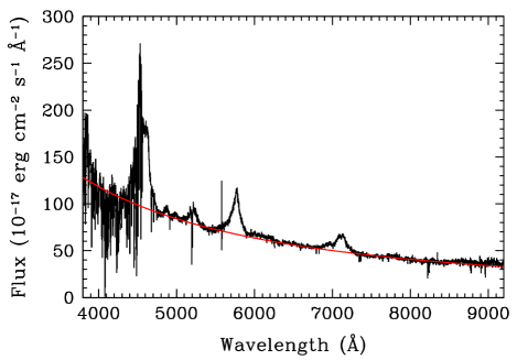
Figure 5: SDSS spectrum of UM 673A,B (black line) together with our power-law fit to the continuum (red line) of the form ${\cal F}_{\lambda}=A\cdot(\lambda/{\rm\AA})^{-\beta}$, with best fitting values $\beta=1.535$ and $A=4.0\times 10^{-10}\,{\rm erg\,s}^{-1}\,{\rm cm}^{-2}\,{\rm\AA}^{-1}$.

5.1 Origin of the Ly$\alpha$ emission

We now discuss some of the mechanisms that could produce the observed Ly$\alpha$ emission, before detailing what we consider to be the most plausible interpretation. The first source we consider is the metagalactic UV background, which could produce Ly$\alpha$ emission by fluorescence, the so-called Hogan-Weymann effect (Hogan & Weymann, 1987). This diffuse emission has yet to be observed, presumably because of the low surface brightness it produces. Given the current understanding of this effect, at the redshift of the DLA we would expect to observe a surface brightness (Gould & Weinberg, 1996),

$$\mu\simeq 5.7\times 10^{-19}\big{(}\frac{\eta_{E}}{0.5}\big{)}\bigg{(}\frac{J}{5.1\times 10^{-22}}\bigg{)}\,\,\,{\rm erg\,s}^{-1}\,{\rm cm}^{-2}\,{\rm arcsec}^{-2},$$ (10)

where $\eta_{E}$ represents the efficiency with which the incident UV background is re-radiated as fluorescent Ly$\alpha$ emission and $J$ is the ionizing background at the Lyman limit at $z\sim 2$ (Bolton et al., 2005). Through the area of sky covered by our observations ($0.86\times 3$ arcsec, the latter being the size of the aperture used to extract the 1-D spectra from the raw 2-D HIRES images), the surface brightness of eq. (10) would produce an integrated line flux $F({\rm Ly\alpha})\sim 1.5\times 10^{-18}\,{\rm erg\,s}^{-1}\,{\rm cm}^{-2}$, one order of magnitude lower than the flux recorded.

Ly$\alpha$ fluorescence can also be induced by the UV radiation from a nearby AGN impinging on the DLA (e.g. Adelberger et al., 2006). Following the formalism introduced by Cantalupo et al. (2005), a source with monochromatic luminosity $L_{\nu}(\nu)\,=\,L_{\nu}(\nu_{\rm LL})\,(\nu/\nu_{\rm LL})^{-\alpha}$, where $h\nu_{\rm LL}=13.6\,{\rm eV}$, at a physical distance $r$ from the DLA will correspond to a “boost factor”

$$\mathcal{B}\,=\,15.2\,\frac{L_{\nu}(\nu_{\rm LL})}{10^{30}\,{\rm erg\,s}^{-1}\,{\rm Hz}^{-1}}\,\frac{0.7}{\alpha}\left(\frac{r}{1\,\,{\rm Mpc}}\right)^{-2}$$ (11)

where, for self-shielded clouds, $\mathcal{B}$ is empirically related to the increase in the observed Ly$\alpha$ surface brightness relative to that induced by the metagalactic UV background, SB(Ly$\alpha$)$/\mu=(0.74+0.50\,\mathcal{B}^{0.89})$. Assuming that the observed Ly$\alpha$ emission is uniform across the area of sky covered by our observations ($0.86\times 3\,{\rm arcsec}$), the corresponding surface brightness is ${\rm SB(Ly}\alpha)=9.7\times 10^{-18}\,{\rm erg\,s}^{-1}\,{\rm cm}^{-2}\,{\rm arcsec}^{-2}$, therefore requiring a boost factor $\mathcal{B}\simeq 50$.

Consider now a typical QSO at $z=1.5-2$, with spectral index $\alpha=1.76$ and $\lambda\,L_{\lambda}(\lambda)=1.5\times 10^{46}\,{\rm erg\,s}^{-1}$ at $1100$ Å (Telfer et al., 2002). One can extrapolate this typical luminosity to the Lyman limit using the relation

$$L_{\nu}(\nu_{\rm LL})=\frac{\lambda_{\rm LL}^{2}}{c}L_{\lambda}(\lambda)\left(\frac{\lambda}{\lambda_{\rm LL}}\right)^{2-\alpha}\approx 4\times 10^{30}\,{\rm erg\,s}^{-1}\,{\rm Hz}^{-1}.$$ (12)

Substituting $\mathcal{B}$, $L_{\nu}(\nu_{\rm LL})$ and $\alpha$ into eq. (11) yields a physical distance $r=700\,{\rm kpc}$. Thus, if the Ly$\alpha$ emission we see in the spectrum of UM 673B were produced by a nearby source of UV photons, such a source would need to be located within $r\sim 700\,{\rm kpc}$ from UM 673, or $\lower 2.15277pt\hbox{$\;\buildrel<\over{\sim}\;$}1.4\,{\rm arcmin}$ in projection on the sky. As we have not identified any such source in our deep galaxy survey of this area of sky, and none have been reported by others, we consider it unlikely that we are observing fluorescent Ly$\alpha$ emission.

Other possibilities have been put forward (e.g. Dijkstra, Haiman, & Spaans, 2006), but all appear less likely than the most straightforward explanation that the Ly$\alpha$ emission we see is produced by recombination in H ii regions ionized by early-type stars in a galaxy presumably associated with the DLA. Adopting the Kennicutt (1998) relationship between star formation rate (SFR) and H$\alpha$ luminosity, and assuming the ratio Ly$\alpha$/H$\alpha\simeq 8.7$ appropriate for case B recombination, yields an equation of the form,

$${\rm SFR}\,\,(M_{\odot}\,{\rm yr}^{-1})=9.1\times 10^{-43}\,L({\rm Ly\alpha})\times\frac{1}{1.8}\,({\rm erg\,s}^{-1}).$$ (13)

where the correction factor of 1/1.8 accounts for the flattening of the stellar initial mass function for masses below $1{\rm M}_{\odot}$ (Chabrier, 2003) compared to the single power law of the Salpeter IMF assumed by Kennicutt (1998).

Thus, our inferred line luminosity, $L({\rm Ly\alpha})=4.3\times 10^{41}\,{\rm erg\,s}^{-1}$ implies a star formation rate ${\rm SFR}\simeq 0.2$ M_⊙ yr^-1. In reality this is likely to be a lower limit, given the ease with which Ly$\alpha$ photons are destroyed through resonant scattering in a dusty medium. In addition, our HIRES slit may have captured only a fraction of the Ly$\alpha$ emission, if it is spatially more extended than the B image of UM 673 (a possibility which we cannot readily assess with our spectroscopic observations). However, we note that such low levels of star formation are not unusual for DLA host galaxies at $z\lower 2.15277pt\hbox{$\;\buildrel<\over{\sim}\;$}1$ (Péroux et al., 2010).

5.2 Lensed Ly$\alpha$ emission?

We next turn to the issue of where the Ly$\alpha$ emitting region is located and whether it too may be lensed by the foreground galaxy at $z=0.493$. Since the angular diameter distances from the lens to UM 673 (1130 Mpc) and from the lens to the absorption system (1036 Mpc) differ by only $\sim 10\%$, we would expect the lensing geometry to be largely unchanged. Thus, presumably the Ly$\alpha$ photons are also lensed by the foreground galaxy into a sister image near to, but offset from, the A sightline. The fact that we do not see any such emission in the core of the damped Ly$\alpha$ absorption line in UM 673A suggests that the HIRES slit was not well placed to capture the A counterpart of the Ly$\alpha$ emission. A more rigorous approach involves detailed modelling of the mass distribution of the foreground lensing galaxy, which unfortunately is not well constrained (Lehár et al., 2000).

We also note that the observed Ly$\alpha$ flux may be slightly magnified, or demagnified, by the foreground galaxy, implying that the intrinsic Ly$\alpha$ luminosity is different from that observed. However, a firm determination of the magnification factor is made difficult by the uncertain mass distribution of the lensing galaxy. Apart from improved modelling of the lens, progress in the interpretation of the Ly$\alpha$ emission would be greatly facilitated by follow-up near-infrared integral field spectroscopy aimed at detecting the redshifted H$\alpha$ emission line at $z=1.62650$. Such observations would map out the full extent of the emission region, without the limitations imposed by single-slit spectroscopy.

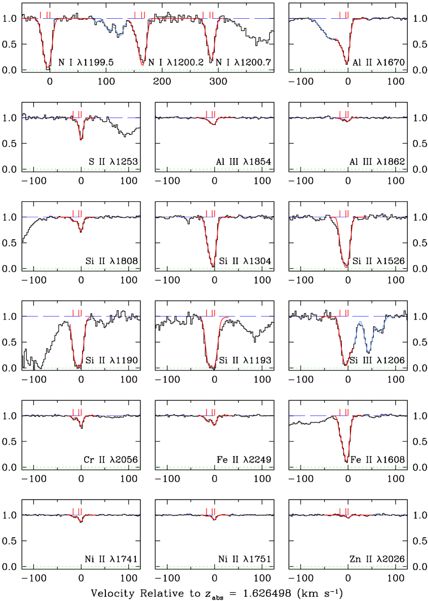
Figure 6: A selection of metal absorption lines associated with the DLA in UM 673A, including transitions from neutral, singly and doubly ionized species. The data are shown as black histograms, while the red continuous lines are profile fits computed with vpfit (see text). A light blue continuous line is used to indicate nearby absorption not associated with the DLA, such as the blue wing of Al ii $\lambda 1670$ (top right-hand panel), which has been included for completeness in the profile fitting procedure. The $y$-axis is residual intensity, and the velocities on the $x$-axis are relative to the redshift of the absorption component with the highest optical depth (component number 3 in Table LABEL:tab:UM673A_lowion_cloudmodel). Vertical tick marks indicate the velocities of the three absorption components producing the absorption lines, with the parameters listed in Table LABEL:tab:UM673A_lowion_cloudmodel.

6 Chemical Composition of the DLA in front of UM 673A

As is normally the case, a multitude of metal absorption lines are associated with the DLA towards UM 673A. With the wide wavelength coverage, high resolution and S/N ratio of our HIRES data, we detect 37 atomic transitions from elements from C to Zn in a variety of ionization stages, from neutrals to triply ionized species, as detailed in Table 2. Although not all of these lines are available for abundance analysis (some being blended or saturated), we nevertheless have at our disposal a great deal of information on the detailed chemical composition of this DLA. In this section, we analyse these data which may throw light on the chemical enrichment history of the galaxy giving rise to the DLA and provide clues to stellar nucleosynthesis at low metallicities.

Table 2: Metal lines detected at the redshift of the DLA in UM 673A

Ion	Wavelengtha	$f^{\rm a}$	$W_{0}^{\rm b}$	$\delta W_{0}^{\rm b}$
	(Å)		(mÅ)	(mÅ)
C ii	1334.5323	0.1278	140	2
C iv	1548.2041	0.1899	…c	…c
C iv	1550.7812	0.09475	73	2
N i	1199.5496	0.132	71	2
N i	1200.2233	0.0869	67	2
N i	1200.7098	0.0432	55	2
O i	1302.1685	0.048	129	2
Al ii	1670.7886	1.740	…c	…c
Al iii	1854.71829	0.559	14.8	0.9
Al iii	1862.79113	0.278	7.6	0.8
Si ii	1190.4158	0.292	89	2
Si ii	1193.2897	0.582	120	2
Si ii	1260.4221	1.18	142	2
Si ii	1304.3702	0.0863	83.1	0.9
Si ii	1526.7070	0.133	118	1
Si ii	1808.01288	0.00208	24.6	0.8
Si iii	1206.500	1.63	…c	…c
Si iv	1393.76018	0.513	…c	…c
Si iv	1402.77291	0.254	…c	…c
S ii	1250.578	0.00543	…c	…c
S ii	1253.805	0.0109	21	1
S ii	1259.518	0.0166	…c	…c
Cr ii	2056.25693	0.103	21.6	0.9
Cr ii	2062.23610	0.0759	14.0	0.8
Cr ii	2066.16403	0.0512	10.3	0.9
Fe ii	1260.533	0.0240	…c	…c
Fe ii	1608.4509	0.0577	94.3	0.8
Fe ii	1611.20034	0.00138	…c	…c
Fe ii	2249.8768	0.001821	24	1
Fe ii	2260.7805	0.00244	32	1
Ni ii	1317.217	0.057	…c	…c
Ni ii	1370.132	0.056	8.4	0.9
Ni ii	1454.842	0.0323	…c	…c
Ni ii	1502.148	0.0133	…c	…c
Ni ii	1741.5531	0.0427	10.3	0.5
Ni ii	1751.9157	0.0277	6.0	0.6
Zn ii	2026.13709	0.501	4.8	0.7

^a Laboratory wavelengths and $f$-values from Morton (2003)

with updates by Jenkins & Tripp (2006).

^b Rest frame equivalent width and error.

^c Blended line.

6.1 Profile Fitting

Fig. 6 shows a selection of metal absorption lines associated with the DLA. The absorption is evidently confined to a narrow velocity range, with even the strongest lines only extending over ${\rm FWHM}\simeq 25$–30 km s^-1. In order to deduce values for the column density $N$ (cm^-2) and velocity dispersion parameter $b$ (km s^-1), we employed the absorption line profile fitting software vpfit, which uses a $\chi^{2}$ minimization technique to fit multiple Voigt profiles simultaneously to several atomic transitions and returns the best fitting values of $N$ and $b$ together with the associated errors (see, for example, Rix et al., 2007). The theoretical line profiles generated by vpfit are superimposed on the data in Fig. 6. We now consider in turn gas of low, intermediate, and high ionization.

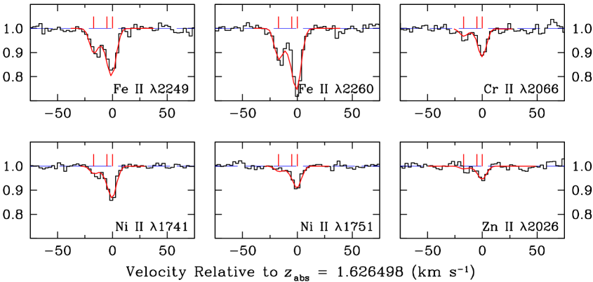
Figure 7: A selection of weak metal absorption lines used for abundance determinations in the DLA in UM 673A, reproduced on an expanded scale. The data are shown as black histograms, while the red continuous lines are profile fits computed with vpfit (see text). The $y$-axis is residual intensity, and the velocities on the $x$-axis are relative to the redshift of the absorption component with the highest optical depth (component number 3 in Table LABEL:tab:UM673A_lowion_cloudmodel). Vertical tick marks indicate the velocities of the three absorption components listed in Table LABEL:tab:UM673A_lowion_cloudmodel.

6.1.1 Low ion transitions

The Si ii, Cr ii, Fe ii and Ni ii lines can all be fitted with a minimum of three absorption components, with the parameters listed in Table LABEL:tab:UM673A_lowion_cloudmodel. The highest optical depth is measured at $z_{\rm abs}=1.626498$ (component number 3 in Table LABEL:tab:UM673A_lowion_cloudmodel, or C3 for short), which we therefore use as the zero point of the relative velocity scale for the DLA. A second component (component number 1, or C1 for short) at $z_{\rm abs}=1.626348$, or $\Delta v=-17.1$ km s^-1, can be readily recognised in the profiles of the weaker lines (e.g. Fe ii $\lambda 2249$) in Fig. 6. What is not immediately obvious from the Figure is that a third component (C2), at $z_{\rm abs}=1.626454$ and separated by only $\Delta v=-5.0$ km s^-1 from C3, is required to reproduce the asymmetric profiles and widths of the stronger lines. Note the small $b$-values, of order 1 km s^-1, deduced for C1 and C3. Although these components are unresolved with the HIRES instrumental resolution of ${\rm FWHM}=8.3$ km s^-1 (Section 2), their narrow widths are indicated by the relative strengths and profiles of Si ii lines of widely differing oscillator strengths. Ultimately, such low velocity dispersions can only be confirmed with higher resolution observations. However, we note that comparably low $b$-values are not unusual in cool clouds in the Milky Way disk and halo (e.g. Pettini, 1988; Barlow et al., 1995), and are now beginning to be measured at high redshifts too as the quality of the spectroscopic data improves (e.g. Jorgenson et al., 2009).

Table 3: Absorption Components of Low Ion Transitions in the DLA in line to UM673A

Comp.	$z_{\rm abs}$	$\Delta v^{\rm a}$	$b$	Fract.b
No.		(km s-1)	(km s-1)
1	$1.626348\pm 2\times 10^{-6}$	$-17.1$	$0.68\pm 0.07$	0.17
2	$1.626454\pm 2\times 10^{-6}$	$-5.0$	$5.9\pm 0.2$	0.25
3	$1.626498\pm 8\times 10^{-6}$	0.0	$1.5\pm 0.3$	0.58

With the redshift $z$ and velocity dispersion parameter $b$ fixed to be the same for all lines of neutral and singly ionized species, we let the column density in each component be the free parameter to be determined by vpfit [with the obvious restriction that all absorption lines arising from the same ground state of a given ion Xn should yield the same value of $N$(Xn)]. Values of $N$(Xn) are collected in Table 4, where the column densities of components C2 and C3 are grouped together, as these two components are always blended at the resolution of our data. We also list in this Table the total (C1+C2+C3) column densities of each ion, which are better determined than those of the individual components.

Table 4: Ion column densities of the DLA in UM673A

Ion	log $N$(X)/${\rm cm}^{-2}$	log $N$(X)/${\rm cm}^{-2}$	log $N$(X)/${\rm cm}^{-2}$
	C1a	C2+C3a	C1+C2+C3a
H i	N/A	N/A	$20.7\pm 0.1$
N i	12.17 $\pm$ 0.41	14.97 $\pm$ 0.25	14.97 $\pm$ 0.25
Al ii	11.91 $\pm$ 0.16	12.89 $\pm$ 0.07	12.93 $\pm$ 0.08
Al iii	11.05 $\pm$ 0.16	11.89 $\pm$ 0.03	11.95 $\pm$ 0.05
Si ii	13.99 $\pm$ 0.07	14.67 $\pm$ 0.02	14.75 $\pm$ 0.03
Si iii	12.32 $\pm$ 0.43	13.05 $\pm$ 0.09	13.12 $\pm$ 0.17
S ii	12.90 $\pm$ 0.43	14.52 $\pm$ 0.09	14.53 $\pm$ 0.10
Ti ii	N/A	N/A	$\leq 11.90^{\rm b}$
Cr ii	12.04 $\pm$ 0.10	12.69 $\pm$ 0.03	12.78 $\pm$ 0.04
Fe ii	14.05 $\pm$ 0.05	14.44 $\pm$ 0.02	14.59 $\pm$ 0.03
Ni ii	12.17 $\pm$ 0.12	12.92 $\pm$ 0.02	12.99 $\pm$ 0.04
Zn ii	10.54 $\pm$ 0.43	11.37 $\pm$ 0.09	11.43 $\pm$ 0.15

^aC1/C2/C3: Component 1/2/3.

^b$3\sigma$ upper limit.

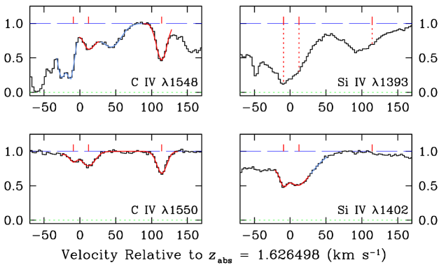
Figure 8: Transitions from highly ionized gas at redshifts close to that of the DLA in UM 673A. In each plot, the $y$-axis is residual intensity, and the velocities on the $x$-axis are relative to the redshift of the absorption component with the highest optical depth in neutral gas (component number 3 in Table LABEL:tab:UM673A_lowion_cloudmodel). The data are shown as black histograms, while the red continuous lines are profile fits computed with the model parameters listed in Table LABEL:tab:UM673A_highion_cloudmodel. A light blue continuous line is used to indicate nearby absorption not associated with the DLA, but which has been included for completeness in the profile fitting procedure. The relative velocities of the three components of the model are indicated by red tick marks above the continuum level. All three components are blended with other absorption lines in Si iv $\lambda 1393$ (top right-hand panel), but component number 3, at $\Delta v=+114$ km s^-1, is clearly absent in Si iv $\lambda 1402$.

It is important to stress in this regard that, with the exception of N i, our data include at least one weak, unsaturated, transition for all of the species used in our abundance determinations. Some examples are shown on an expanded scale in Fig. 7. Under these circumstances, the values of column density deduced do not depend on the details of the profile fitting, because the lines lie on the linear part of the curve of growth. Although we record C ii $\lambda 1334$ and O i $\lambda 1302$, these transitions are saturated; these species are therefore not included in Table 4 and in the subsequent abundance analysis. We do however include Ti ii, whose $\lambda\lambda 1910.61,1910.95$ doublet is undetected; the $3\sigma$ upper limit $\log[N$(Ti ii)/cm${}^{-2}]\leq 11.90$ in Table 4 was deduced assuming these lines to be as wide as Zn ii $\lambda 2026$, which is the weakest feature we detect.

The column densities of the neutrals and first ions in Table 4 allow us to deduce directly the abundances of the corresponding elements. Before doing so in Section 6.2 below, we briefly comment on the absorption from more highly ionized gas.

Table 5: Absorption Components of High Ion Transitions at Redshifts Close to That of the DLA in UM 673A

Comp.	$z_{\rm abs}$	$\Delta v^{\rm a}$	$b$	Fract.b
No.		(km s-1)	(km s-1)
1	$1.626416\pm 3\times 10^{-6}$	$-9.4$	$4.2\pm 0.9$	0.51
2	$1.626605\pm 3\times 10^{-6}$	$+12.2$	$11.4\pm 0.7$	0.11
3	$1.627498\pm 2\times 10^{-6}$	$+114.1$	$7.9\pm 0.3$	0.38

6.1.2 Intermediate ionization stages

Our data cover two second ions, Al iii $\lambda\lambda 1854,1862$ and Si iii $\lambda 1206$; all three transitions are shown in Fig. 6. The weak Al iii doublet lines are well reproduced by the same ‘cloud model’ determined for the low ionization species (Table LABEL:tab:UM673A_lowion_cloudmodel). The stronger Si iii $\lambda 1206$ line shows additional redshifted absorption which presumably arises in ionized gas, since it is absent from lines of comparable strength of ions which are dominant in H i regions (e.g. Si ii $\lambda 1526$—see Fig. 6). Accordingly, the column densities of Al iii and Si iii listed in Table 4 refer only to the velocity interval appropriate to the neutral gas. These values of column densities are useful for constraining the magnitude of putative ionization corrections to the abundance determinations, as discussed in Appendix A.

Table 6: High Ion Column Densities at Redshifts Close to That of the DLA in UM 673A

Ion	log $N$(X)/${\rm cm}^{-2}$	log $N$(X)/${\rm cm}^{-2}$	log $N$(X)/${\rm cm}^{-2}$
	C1a	C2a	C3a
C iv	12.55 $\pm$ 0.06	13.10 $\pm$ 0.02	13.22 $\pm$ 0.01
Si iv	$12.59^{\rm b}$	$12.45^{\rm b}$	$\leq 11.75^{\rm c}$

^aC1/C2/C3: Component 1/2/3.

^bUncertain because of blending.

^c$3\sigma$ upper limit.

6.1.3 High ions

We also find lines from highly ionized gas at redshifts close to, but not the same as, that of the DLA. The extensive work by Fox et al. (2007) has shown this to be the case in many DLAs. Our HIRES spectrum includes absorption lines from the C iv $\lambda\lambda 1548,1550$ and Si iv $\lambda\lambda 1393,1402$ doublets, although out of these four lines only C iv $\lambda 1550$ is not blended and therefore affords the clearest view of the kinematic structure of the highly ionized gas (see Fig. 8).

The highly ionized gas appears to be spread over three velocity components (Table LABEL:tab:UM673A_highion_cloudmodel); two are close in redshift to the DLA itself ($\Delta v=-9.4$ and +12.2 km s^-1 respectively for components 1 and 2 in Table LABEL:tab:UM673A_highion_cloudmodel), but the third is redshifted by $\Delta v=+114$ km s^-1. This third component must be of high ionization indeed, as it is the strongest in C iv and yet is absent in Si iv (see Fig. 8). Comparison of the $b$-values in Tables LABEL:tab:UM673A_highion_cloudmodel and LABEL:tab:UM673A_lowion_cloudmodel shows that the high ions have larger velocity dispersions than the neutral gas. Table 6 lists the column densities of C iv and Si iv.

Comparing Fig. 8 with the lower three panels of Fig. 2, it can be readily appreciated that, in stark contrast with the low ion absorption lines, the C iv  and Si iv  absorption lines show little variation between UM 673A and B. Applying the same vpfit analysis as above to the C iv lines in UM 673B, returns values of redshift for the three absorption components which differ by less than 5 km s^-1 from those listed in Table LABEL:tab:UM673A_highion_cloudmodel, and values of column density $N$(C iv) which differ by less than a factor of 3 from those listed in Table 6. The finding that highly ionized gas has a much larger coherence scale than that of DLAs is not surprising, and in line with the results of earlier work on other QSO pairs (e.g. Rauch et al., 2001; Ellison et al., 2004, and references therein) and more recently on galaxy-galaxy pairs (Steidel et al., 2010).

6.2 Element Abundances

Abundance measurements for the DLA in UM 673A are collected in Table 7 and shown graphically in Fig. 9. These values were deduced directly by dividing the column densities of ions which are dominant in H i regions by $N$(H i) (see Table 4), with the implicit assumption that corrections for ionized gas and unseen ion stages are negligible so that, for example, $N({\rm Si\,\textsc{ii}})/N(\textrm{H}\,\textsc{i})\equiv{\rm Si/H}$. The validity of this assumption is examined in Appendix A, with the conclusion that it is likely to be accurate to within $\sim 0.05$ dex for most elements considered here, except Al and S, whose true abundances may be higher than their entries in Table 7 by 0.1 dex and 0.2 dex respectively. We used as reference the compilation of solar abundances by Asplund et al. (2005); the very recent revision of the solar scale by Asplund et al. (2009) differs for the elements listed in Table 7 by at most 0.05 dex (for N) and more generally by only 0.02–0.03 dex.

The first conclusion to be drawn from Fig. 9 is that the $z=1.62650$ DLA in line to UM 673A is metal-poor, with an overall metallicity $Z\simeq 1/30Z_{\odot}$, or $-1.5$ on a log scale. Such low metallicity is not unexpected, given the narrow widths of the absorption lines (which are actually significantly narrower than expected on the basis of the relationship proposed by Prochaska et al., 2008) and the apparently low level of star formation deduced in Section 5.

Table 7: Element Abundances in the DLA at $z_{\rm abs}=1.626498$ towards UM 673A

Element	log (X/H)${}_{\odot}^{\rm a}$	[X/H]${}_{\rm DLA}^{\rm b}$
(X)
N	$-4.22$	$-1.51\pm 0.25$
Al	$-5.57$	$-2.20\pm 0.08$
Si	$-4.49$	$-1.46\pm 0.03$
S	$-4.86$	$-1.31\pm 0.10$
Ti	$-7.10$	$<-1.70$
Cr	$-6.36$	$-1.56\pm 0.04$
Fe	$-4.55$	$-1.56\pm 0.03$
Ni	$-5.77$	$-1.94\pm 0.04$
Zn	$-7.40$	$-1.87\pm 0.15$

^aAsplund et al. (2005)

^b$[{\rm X}/{\rm H}]_{\rm DLA}\equiv\log({\rm X}/{\rm H})_{\rm DLA}-\log({\rm X}/{\rm H})_{\odot}$

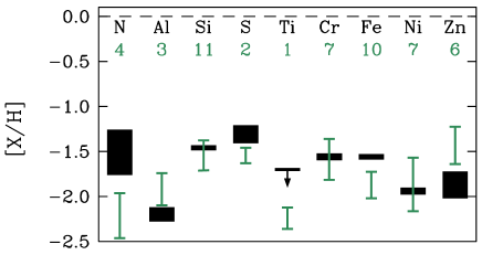
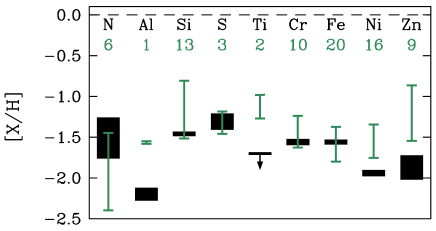
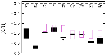
Figure 9: All three panels show the abundances of the nine elements indicated at the top in the $z_{\rm abs}=1.62650$ DLA in front of UM 673A (black boxes); the size of each box corresponds to the uncertainty in each determination (except for Ti, for which we only have an upper limit). The green vertical lines in the top and middle panels show the dispersions of the abundances of each element in samples of DLAs that have, respectively, [Si/H] and [Fe/H] within a factor of 2 of the DLA in UM 673A. The numbers below the element tags indicate the number of DLA measurements available for each element (see text for further details). In the bottom panel the DLA chemical composition is compared with that of an ‘average’ population of Galactic metal-poor stars (open boxes) that have [Fe/H] within a factor of 2 of the DLA.

When we look more closely at the relative abundances of the elements measured, however, we arrive at the interesting conclusion that this DLA exhibits some notable differences from the ‘average’ populations of DLAs and Galactic halo stars of similar metallicity, as we now point out. We consider two ‘average’ sets of DLAs, each assembled from the HIRES DLA database compiled by Prochaska et al. (2007). In each case we selected from the database all DLAs whose abundance is within a factor of 2 of a reference element, using in turn Si and Fe as the reference. Thus, the green vertical lines in the top panel of Fig. 9 show the dispersion in the abundances of the elements considered here in all DLAs with $-1.76\leq{\rm[Si/H]}\leq-1.16$, i.e. within a factor of $\sim 2$ of the value ${\rm[Si/H]}=-1.46\pm 0.03$ we measure towards UM 673A. The middle panel shows the same data for all DLAs with $-1.86\leq{\rm[Fe/H]}\leq-1.26$. The numbers below the element tags in Fig. 9 indicate the number of DLAs included in the average population for the corresponding element. If there exists only one measurement, the size of the error bar represents the uncertainty in that single measurement. If just two or three measurements exist, we instead plot the standard error in the mean. Otherwise, we use a robust determination of the dispersion in the average population (see Section 4).

Similarly, in the bottom panel of Fig. 9, we overlay (empty boxes) the element abundances of the average population of Galactic metal poor stars drawn from the samples of Gratton et al. (2003) and Nissen et al. (2007), using Fe as the reference element. For all available measurements, the height of the box represents the dispersion in the average population.

Considering first the top panel of Fig. 9, it appears that the DLA in UM 673A is Fe-rich and Zn-poor relative to other DLAs with similar Si abundance. There may be offsets in N and S too, but their statistics are poorer. The best DLA statistics are those for the middle panel, where we see that, relative to other DLAs with similar Fe abundance, the absorber in UM 673A is deficient in Ti, Ni, and Zn. The same conclusion is reached by comparing with the stellar abundances in the bottom panel.

It seems unlikely that these apparently anomalous abundances are due to dust depletion, given that: (a) Ti, Ni, and Zn are depleted to very different degrees in Galactic dust (Savage & Sembach, 1996), and (b) depletions are in any case expected to introduce very minor corrections when the overall metallicity is as low as 1/30 of solar (e.g. Akerman et al., 2005).

The unusually low abundance of Zn (an element which is not readily incorporated into dust grains and thus normally provides a reliable benchmark for the abundance of Fe-peak elements, e.g. Pettini et al., 1990), can best be appreciated from Fig. 10, where the value of [Zn/Fe] in UM 673A is compared with those measured in DLAs and Galactic stars. In the Figure, the trend of decreasing [Zn/Fe] with decreasing [Zn/H] in DLAs is most naturally explained by the reduced dust depletion of Fe at lower metallicities, until solar relative abundance of the two elements is recovered when ${\rm[Zn/H]}\simeq-1.5$. In Galactic stars, Zn and Fe track each other closely over two decades in metallicity (from solar to $\sim 1/100$ solar), and Zn becomes progressively overabundant relative to Fe with decreasing metallicity when [Zn/H] $\lower 2.15277pt\hbox{$\;\buildrel<\over{\sim}\;$}-2$. Evidently, the [Zn/Fe] ratio is lower in UM 673A than in any other DLA in current samples; similarly, none of the metal-poor stars in the compilations by Nissen et al. (2007) and Saito et al. (2009) exhibits an underabundance of Zn relative to Fe as pronounced as that uncovered here.

We have searched for clues in the composition of Galactic stars that are much more metal-poor than 1/30 of solar, in the extreme regime where chemical anomalies due to enrichment by only a few prior episodes of star formation may manifest themselves, but found none. The works by Cayrel et al. (2004) and Lai et al. (2008) show that when ${\rm Fe/H}\ll-2$, Ti is overabundant by a factor of $\sim 2$ relative to Fe, Cr is progressively underabundant with decreasing [Fe/H], Ni/Fe remains solar, and Zn exhibits the behaviour illustrated in Fig. 10, quite unlike the relative abundances of these four elements relative to Fe in the DLA towards UM 673A.

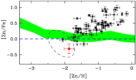
Figure 10: Zn and Fe abundances in DLAs from the compilations by Prochaska et al. (2007), Dessauges-Zavadsky et al. (2007), and Noterdaeme et al. (2008) are shown with black circles, while the red dot is for the DLA in UM 673A. Note that the fall off in [Zn/Fe] with decreasing [Zn/H] in DLAs is not thought to be intrinsic, but rather to reflect a decreasing fraction of Fe in dust grains at lower overall metallicities, as measured by the normally undepleted Zn. The green shaded region shows the behaviour of [Zn/Fe] in Galactic stars (Saito et al., 2009, and references therein), with the width of the band corresponding to the $\pm 1\sigma$ dispersion of values at a given metallicity. The dashed ellipse indicates the approximate locus of stars in the dwarf spheroidal galaxies Draco, Ursa Minor, and Sextans from the work by Shetrone, Côté, & Sargent (2001) and Cohen & Huang (2009).

Recently, data have become available on the abundances of these elements in individual stars of dwarf spheroidal galaxies in the Local Group (Shetrone, Côté, & Sargent, 2001; Cohen & Huang, 2009) and in ultra-faint dwarf companions of the Milky Way (Frebel et al., 2010). These measurements are of particular interest, as some of these galaxies may well have experienced different star formation histories from the stellar population(s) of the Galactic halo, and may therefore offer a different perspective for the interpretation of element ratios. It is thus intriguing to find that stars with [Fe/H] $\lower 2.15277pt\hbox{$\;\buildrel<\over{\sim}\;$}-2$ in the Draco, Sextans, and Ursa Minor dwarf spheroidal galaxies can exhibit sub-solar [Zn/Fe] ratios (see Fig. 10), and solar or sub-solar [Ti/Fe] (in contrast with the super-solar [Ti/Fe] of Galactic halo stars). However, the resemblance to the DLA in UM 673A does not extend to other elements: in the dwarf spheroidal stars observed by Shetrone, Côté, & Sargent (2001) and Cohen & Huang (2009) the mean value of [Ni/Fe] is approximately solar and [Cr/Fe] is mostly subsolar, whereas the opposite is found in the DLA (see Fig. 9). Thus, while these data do offer examples of clear departures of some element ratios from the well-established Galactic halo pattern, a definite chemical correspondence between the DLA in UM 673A and nearby dwarf spheroidal galaxies cannot be established.

It is possible that, as more data of comparably high S/N ratio to those presented here are obtained for other very metal-poor DLAs, more examples of anomalous element abundances will be uncovered, challenging current calculations of stellar yields at low metallicities. Sub-solar [Zn,Ni,Ti/Fe] ratios in very metal-poor DLAs may well be more common than has been appreciated so far, because the absorption lines of all three elements become vanishingly small when [Fe/H] $\lower 2.15277pt\hbox{$\;\buildrel<\over{\sim}\;$}-1.5$ (see, for example, Pettini et al., 2008a), requiring data of unusually high S/N ratio for their abundances to be determined.

7 Summary and Conclusions

Thanks to the high efficiency of the HIRES spectrograph at ultraviolet wavelengths, we have uncovered a damped Ly$\alpha$ system at $z=1.62650$ in the spectrum of the gravitationally lensed QSO UM 673; the DLA had been overlooked until now, despite the many observations of this bright QSO over the last quarter of a century. From the analysis of high resolution and S/N ratio spectra of each image of the UM 673A,B pair, we draw the following conclusions.

(i) In the direction probed, the transverse extent of the DLA is much less than 2.7 kpc (this being the separation of the two sightlines at $z=1.62650$), since we measure a drop by a factor of at least 400 in the column density of neutral hydrogen from UM 673A ($\log[N$(H i)/cm${}^{-2}]=20.7$) to UM 673B ($\log[N$(H i)/cm${}^{-2}]\leq 18.1$). A comparable drop is seen in the column density of Si ii and presumably other metals in stages that are dominant in H i regions.

(ii) From a reassessment of data on other QSO pairs in the literature, together with the new results for UM 673A,B, we find that, if the radial profile of $N$(H i) in DLAs declines exponentially, the median $e$-folding scale length is $\tilde{\rm S}_{\rm DLA,e}=1.3\pm 0.8\,{\rm kpc}$, smaller than had previously been realised. For a spherical cloud, this corresponds to a typical DLA radius $R\simeq 5\pm 3$ kpc.

(iii) Towards UM 673B, we detect a weak and narrow Ly$\alpha$ emission line at the same redshift as the DLA in UM 673A. If the line is due to recombination in H ii regions, which we consider to be the most likely interpretation, its low luminosity ($L({\rm Ly\alpha})=4.3\times 10^{41}\,{\rm erg\,s}^{-1}$) implies a modest star formation rate, ${\rm SFR}\simeq 0.2$ M_⊙ yr^-1. However, this is probably a lower limit considering: (a) the ease with which resonant Ly$\alpha$ photons can be destroyed or scattered out of the line of sight, and (b) the limited spatial sampling of the narrow HIRES entrance slit.

(iv) In contrast with neutral gas, absorption by C iv exhibits only modest variations between the two sightlines. Evidently, highly ionized gas extends over much larger physical dimensions than the DLA, in accord with earlier conclusions from other QSO pairs and recent work on galaxy-galaxy pairs.

(v) The DLA in front of UM 673A is metal poor, with overall metallicity $Z_{\rm DLA}\simeq 1/30Z_{\odot}$, and has a very simple velocity structure, with three absorption components spread over a narrow velocity interval, $\Delta v=17$ km s^-1. Two of the components have very small internal velocity dispersions, with $b=\sqrt{2}\sigma\simeq 1$ km s^-1, where $\sigma$ is the one-dimensional rms velocity of the absorbing ions projected along the light of sight.

(vi) We are able to determine with precision the relative abundances of nine chemical elements, from N to Zn, thanks to the large number of metal absorption lines recorded at high S/N ratio. There appear to be some peculiarities in the detailed chemical make-up of the DLA, with the elements Ti, Ni, and Zn being deficient by factors of $\sim 2$–3 compared to other DLAs and to Galactic halo stars of similar overall metallicity. The [Zn/Fe] ratio is the lowest measured in existing samples of DLAs and halo stars. While comparably low values of [Zn/Fe] have been measured in some stars of nearby dwarf spheroidal galaxies, other element ratios differ between these stars and the DLA, so that a direct chemical correspondence cannot be established. An interpretation of these peculiar element ratios in terms of the previous history of chemical enrichment of the gas is still lacking.

Taken together, the small size, quiescent kinematics, and near-pristine chemical composition of the DLA in front of UM 673A would suggest an origin in a low-mass galaxy. However, the detection of nearby Ly$\alpha$ emission adds a new ‘twist’ to this picture. Although not intersected by our line of sight, there must presumably be a significant mass of cold gas within $\sim 3$  kpc of the DLA to fuel the star formation rate we deduce from the Ly$\alpha$ luminosity. If this is the case, then the properties we measure may refer to an interstellar cloud—or complex of clouds—within a larger galaxy, rather than being representative of the whole galaxy. This caveat may also apply to other DLAs whose transverse dimensions have been probed with QSO pairs. However, the fact that in none of the cases studied so far has common DLA absorption been found over scales of a few kpc (see Table 1) points to one (or both) of two possibilities: either interstellar clouds with $N$(H i) $\geq 2\times 10^{20}$ cm^-2 have covering fractions $f_{\rm c}\ll 1$ within the interstellar media of high redshift galaxies or, if $f_{\rm c}\sim 1$, the host galaxies of most DLAs are genuinely of small extent. The generally low metallicities of most DLAs independently point to an origin in low luminosity galaxies as discussed, among others, by Fynbo et al. (2008).

Looking ahead, the nature of the DLA studied here would undoubtedly be clarified by integral field observations of UM 673 at the wavelength of the H$\alpha$ emission line (which at $z=1.62650$ is redshifted into the near-infrared $H$-band, at $\lambda_{\rm obs}=1.7241\,\mu$m). Its detection would confirm the presence of a star-forming region, its spatial extent, and whether or not it is lensed by the foreground galaxy. As a closing remark, we also point out that, with its narrow velocity width and low metallicity, the DLA in UM 673A is a prime candidate for a rare measurement of the primordial D/H ratio (Pettini et al., 2008b). Such data, however, can only be obtained with the Hubble Space Telescope because the higher order Lyman lines in which the isotope shift could be resolved all lie at ultraviolet wavelengths inaccessible from the ground.

Appendix A Ionization Corrections

In Section 6.2 we determined the chemical composition of the DLA by assuming that the ion stage which is dominant in H i regions could be taken to represent the total column density of the corresponding element in the DLA. This is normally a safe assumption at the high neutral hydrogen column densities of DLAs, where the gas is self-shielded from ionizing radiation (e.g. Vladilo et al., 2001). However, given the unusual abundance pattern uncovered here, it is worthwhile reexamining the assumption that, for example, $N{\rm(N\,\textsc{i})}/N{\rm(\textrm{H}\,\textsc{i})}\equiv{\rm N/H}$, and assess to what degree, if any, N may be over- or under-ionized compared to H (and the same for the other elements considered).

To this end, we ran a suite of cloudy photoionization models (Ferland et al., 1998), assuming that the DLA can be approximated by a slab of constant density gas in the range $-3<\log[n({\rm H})/{\rm cm}^{-3}]<3$. In our simulations, we included the Haardt & Madau (2001) metagalactic ionizing background, as well as the cosmic microwave background, both at the redshift of the DLA. We adopted the solar abundance scale of Asplund et al. (2005) and globally scaled the metals to $Z_{\rm DLA}=1/30Z_{\odot}$. No relative element depletions were employed, nor were grains added. The simulations were stopped when the column density of the DLA was reached. We are then able to calculate the ionization correction, IC(X), for element X in ionization stage n by the relation

$$\mathrm{IC(X)}=\log\bigg{[}\frac{N(\mathrm{X})}{N(\mathrm{H})}\bigg{]}_{\mathrm{intrinsic}}-\log\bigg{[}\frac{N(\mathrm{X}\,\textsc{n})}{N(\mathrm{H}\,\textsc{i})}\bigg{]}_{\mathrm{computed}}\,\,\,$$ (14)

which will be negative if we overestimate the abundance of an element by assuming that the dominant ionization stage is representative of the true abundance.

The results of this exercise are shown in Fig. 11, where it can be seen (top panel) that the ionization corrections are less than 0.1 dex for most elements considered, for gas densities in excess of $\log[n{\rm(H)/cm}^{-3}]=-2$. We can constrain the density by considering the relative column densities of successive ion stages, in our case using the Al iii/Al ii and Si iii/Si ii pairs. As can be seen from the bottom panel in Fig. 11, both ratios give consistent answers, indicating a density $\log[n{\rm(H)/cm}^{-3}]=-1.1\pm 0.1$ (from the better determined Si iii/Si ii ratio). At these densities, the ionization corrections for the elements in question are smaller than the uncertainties in the corresponding ion’s column densities (shown by the height of the black boxes in Fig. 9), and can thus be safely neglected. The same conclusion is reached if the radiation field responsible for ionizing the gas has a purely stellar origin, rather than the mix of Active Galactic Nuclei and star-forming galaxies that is the source of the metagalactic background considered by Haardt & Madau (2001).

We can estimate the line-of-sight distance through the DLA, ${\rm D}_{\rm los}$, from our derived volume density under the assumption of constant density [i.e. ${\rm D}_{\rm los}=N({\rm H}\,\textsc{i})/n({\rm H})$]. We find ${\rm D}_{\rm los}=2.1_{-0.7}^{+1.0}\,{\rm kpc}$, consistent with the absence of the DLA in UM 673B and in agreement with the characteristic sizes deduced from our analysis in Section 4.

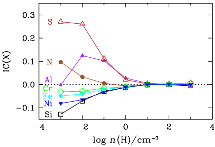
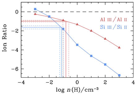
Figure 11: Top: Ionization corrections, as defined by Eq. 14, as a function of the gas density, $n$(H), calculated by cloudy for the elements of interest (see text for further details of the calculations). Bottom: Ratios of successive ion stages of Si and Al (symbols connected by solid lines), as a function of $n$(H). The values of these ratios measured in the DLA are indicated with straight lines; the dotted lines show the corresponding uncertainties.

References

- Adelberger et al. (2005) Adelberger K. L., Shapley A. E., Steidel C. C., Pettini M., Erb D. K., Reddy N. A., 2005, ApJ, 629, 636
- Adelberger et al. (2006) Adelberger, K. L., Steidel, C. C., Kollmeier, J. A., & Reddy, N. A. 2006, ApJ, 637, 74
- Akerman et al. (2005) Akerman C. J., Ellison S. L., Pettini M., Steidel C. C., 2005, A&A, 440, 499
- Asplund et al. (2005) Asplund, M. Grevesse, N. & Sauval, A. J. 2005, in “Cosmic Abundances as Records of Stellar Evolution and Nucleosynthesis, ASP Conf. Series”, ed. T. G. Barnes III & F. N. Bash, (San Francisco: Astron. Soc. Pac.) 336, 25
- Asplund et al. (2009) Asplund, M., Grevesse, N., Sauval, A. J., & Scott, P. 2009, ARAA, 47, 481
- Barlow et al. (1995) Barlow, M. J., Crawford, I. A., Diego, F., Dryburgh, M., Fish, A. C., Howarth, I. D., Spyromilio, J., & Walker, D. D. 1995, MNRAS, 272, 333
- Bolton et al. (2005) Bolton J. S., Haehnelt M. G., Viel M., Springel V., 2005, MNRAS, 357, 1178
- Cantalupo et al. (2005) Cantalupo S., Porciani C., Lilly S. J., Miniati F., 2005, ApJ, 628, 61
- Cayrel et al. (2004) Cayrel, R., et al. 2004, A&A, 416, 1117
- Chabrier (2003) Chabrier, G. 2003, PASP, 115, 763
- Christensen et al. (2007) Christensen L., Wisotzki L., Roth M. M., Sánchez S. F., Kelz A., Jahnke K., 2007, A&A, 468, 587
- Cohen & Huang (2009) Cohen J. G., Huang W., 2009, ApJ, 701, 1053
- Dessauges-Zavadsky et al. (2007) Dessauges-Zavadsky M., Calura F., Prochaska J. X., D’Odorico S., Matteucci F., 2007, A&A, 470, 431
- Dijkstra, Haiman, & Spaans (2006) Dijkstra M., Haiman Z., Spaans M., 2006, ApJ, 649, 14
- Ellison et al. (2004) Ellison, S. L., Ibata, R., Pettini, M., Lewis, G. F., Aracil, B., Petitjean, P., & Srianand, R. 2004, A&A, 414, 79
- Ellison et al. (2007) Ellison S. L., Hennawi J. F., Martin C. L., Sommer-Larsen J., 2007, MNRAS, 378, 801
- Ferland et al. (1998) Ferland G. J., Korista K. T., Verner D. A., Ferguson J. W., Kingdon J. B., Verner E. M., 1998, PASP, 110, 761
- Foltz et al. (1984) Foltz, C. B., Weymann, R. J., Roser, H.-J., & Chaffee, F. H., Jr. 1984, ApJ, 281, L1
- Fox et al. (2007) Fox, A. J., Ledoux, C., Petitjean, P., & Srianand, R. 2007, A&A, 473, 791
- Frebel et al. (2010) Frebel A., Simon J. D., Geha M., Willman B., 2010, ApJ, 708, 560
- Fynbo et al. (2008) Fynbo, J. P. U., Prochaska, J. X., Sommer-Larsen, J., Dessauges-Zavadsky, M., & Møller, P. 2008, ApJ, 683, 321
- Gould & Weinberg (1996) Gould A., Weinberg D. H., 1996, ApJ, 468, 462
- Gratton et al. (2003) Gratton R. G., Carretta E., Claudi R., Lucatello S., Barbieri M., 2003, A&A, 404, 187
- Haardt & Madau (2001) Haardt F., Madau P., 2001, in Neumann D. M., Tran J. T. V., eds, Clusters of Galaxies and the High Redshift Universe Observed in X-ray, preprint (astro-ph/0106018)
- Hoaglin, Mosteller, & Tukey (1983) Hoaglin D. C., Mosteller F., Tukey J. W., 1983, Understanding robust and exploratory data analysis. John Wiley & Sons, New York
- Hogan & Weymann (1987) Hogan C. J., Weymann R. J., 1987, MNRAS, 225, 1P
- Hogg (1999) Hogg, D. W. 1999, arXiv:9905115
- Hunstead et al. (1990) Hunstead R. W., Pettini M., Fletcher A. B., 1990, ApJ, 356, 23
- Jenkins & Tripp (2006) Jenkins, E. B., & Tripp, T. M. 2006, ApJ, 637, 548
- Jorgenson et al. (2009) Jorgenson, R. A., Wolfe, A. M., Prochaska, J. X., & Carswell, R. F. 2009, ApJ, 704, 247
- Kennicutt (1998) Kennicutt R. C., Jr., 1998, ARA&A, 36, 189
- Kneib et al. (1998) Kneib J.-P., Alloin D., Pello R., 1998, A&A, 339, L65
- Kulkarni et al. (2006) Kulkarni V. P., Woodgate B. E., York D. G., Thatte D. G., Meiring J., Palunas P., Wassell E., 2006, ApJ, 636, 30
- Lai et al. (2008) Lai, D. K., Bolte, M., Johnson, J. A., Lucatello, S., Heger, A., & Woosley, S. E. 2008, ApJ, 681, 1524
- Lehár et al. (2000) Lehár J., et al., 2000, ApJ, 536, 584
- MacLeod et al. (2009) MacLeod C. L., Kochanek C. S., Agol E., 2009, ApJ, 699, 1578
- Monier et al. (2009) Monier E. M., Turnshek D. A., Rao S., 2009, MNRAS, 397, 943
- Morton (2003) Morton, D. C. 2003, ApJS, 149, 205
- Nissen et al. (2007) Nissen P. E., Akerman C., Asplund M., Fabbian D., Kerber F., Kaufl H. U., Pettini M., 2007, A&A, 469, 319
- Noterdaeme et al. (2008) Noterdaeme P., Ledoux C., Petitjean P., Srianand R., 2008, A&A, 481, 327
- O’Meara et al. (2007) O’Meara, J. M., Prochaska, J. X., Burles, S., Prochter, G., Bernstein, R. A., & Burgess, K. M. 2007, ApJ, 656, 666
- Péroux et al. (2010) Péroux C., Bouché, N., Kulkarni, V.P., York, D.G., Vladilo, G. 2010, MNRAS, submitted
- Pettini (1988) Pettini, M. 1988, Proceedings of the Astronomical Society of Australia, 7, 527
- Pettini (2006) Pettini, M. 2006, in LeBrun V., Mazure A., Arnouts S. & Burgarella D., eds., The Fabulous Destiny of Galaxies: Bridging Past and Present. Frontier Group, Paris, p. 319 (astro-ph/0603066).
- Pettini et al. (1990) Pettini, M., Boksenberg, A., & Hunstead, R. W. 1990, ApJ, 348, 48
- Pettini et al. (2008a) Pettini M., Zych B. J., Steidel C. C., Chaffee F. H., 2008a, MNRAS, 385, 2011
- Pettini et al. (2008b) Pettini M., Zych B., Murphy, M. T., Lewis, A., & Steidel, C. C., 2008b, MNRAS, 391, 1499
- Prochaska et al. (2007) Prochaska J. X., Wolfe A. M., Howk J. C., Gawiser E., Burles S. M., Cooke J., 2007, ApJS, 171, 29
- Prochaska et al. (2008) Prochaska, J. X., Chen, H.-W., Wolfe, A. M., Dessauges-Zavadsky, M., & Bloom, J. S. 2008, ApJ, 672, 59
- Rauch et al. (2001) Rauch, M., Sargent, W. L. W., & Barlow, T. A. 2001, ApJ, 554, 823
- Rauch et al. (2008) Rauch M., et al., 2008, ApJ, 681, 856
- Rix et al. (2007) Rix, S. A., Pettini, M., Steidel, C. C., Reddy, N. A., Adelberger, K. L., Erb, D. K., & Shapley, A. E. 2007, ApJ, 670, 15
- Saito et al. (2009) Saito Y.-J., Takada-Hidai M., Honda S., Takeda Y., 2009, PASJ, 61, 549
- Sargent et al. (1982) Sargent, W. L. W., Young, P., & Schneider, D. P. 1982, ApJ, 256, 374
- Savage & Sembach (1996) Savage, B. D., & Sembach, K. R. 1996, ARAA, 34, 279
- Schneider et al. (2007) Schneider D. P., et al., 2007, AJ, 134, 102
- Shetrone, Côté, & Sargent (2001) Shetrone M. D., Côté P., Sargent W. L. W., 2001, ApJ, 548, 592
- Smette et al. (1992) Smette A., Surdej J., Shaver P. A., Foltz C. B., Chaffee F. H., Weymann R. J., Williams R. E., Magain P., 1992, ApJ, 389, 39
- Steidel et al. (2010) Steidel C. C., Erb D. K., Shapley A. E., Pettini M., Reddy N., Bogosavljević M., Rudie G. C., Rakic O., 2010, ApJ, 717, 289
- Storrie-Lombardi & Wolfe (2000) Storrie-Lombardi, L. J., & Wolfe, A. M. 2000, ApJ, 543, 552
- Surdej et al. (1987) Surdej J., et al., 1987, Nature, 329, 695
- Surdej et al. (1988) Surdej J., et al., 1988, A&A, 198, 49
- Telfer et al. (2002) Telfer R. C., Zheng W., Kriss G. A., Davidsen A. F., 2002, ApJ, 565, 773
- Vladilo et al. (2001) Vladilo, G., Centurión, M., Bonifacio, P., & Howk, J. C. 2001, ApJ, 557, 1007
- Vogt et al. (1994) Vogt S. S., et al., 1994, SPIE, 2198, 362
- Wolfe & Chen (2006) Wolfe, A. M., & Chen, H.-W. 2006, ApJ, 652, 981
- Wolfe et al. (2005) Wolfe, A. M. Gawiser, E. & Prochaska, J. X. 2005, ARA&A, 43, 861