On the range of a random walk in a torus and random interlacements

Abstract

Let a simple random walk run inside a torus of dimension three or higher for a number of steps which is a constant proportion of the volume. We examine geometric properties of the range, the random subgraph induced by the set of vertices visited by the walk. Distance and mixing bounds for the typical range are proven that are a $k$-iterated log factor from those on the full torus for arbitrary $k$. The proof uses hierarchical renormalization and techniques that can possibly be applied to other random processes in the Euclidean lattice. We use the same technique to bound the heat kernel of a random walk on random interlacements.

and

t1Work on this project was done while the author was in the Weizmann Institute of Science. T2Supported by ISF Grant 1300/08 and EU Grant PIRG04-GA-2008-239317.

1 Introduction

Consider a discrete torus of side length $N$ in dimension $d\geq 3$. Let a simple random walk run in the torus until it fills a constant proportion of the torus and examine the range, the random subgraph induced by the set of vertices visited by the walk. How well does this range capture the geometry of the torus? Viewing the range as a random perturbation of the torus, we can draw hope that at least some geometric properties of the torus are retained, by considering results on a more elementary random perturbation, Bernoulli percolation.

It is now known that various properties of the Euclidean lattice “survive” Bernoulli percolation with density $p>p_{c}(\mathbb{Z}^{d})$. In antal1996chemical , Antal and Pisztora proved that there is a finite $C(p,d)$ such that the graph distance between any two vertices in the infinite cluster is more than $C$ times their $l_{2}$ distance, with probability exponentially low in this distance. Isoperimetric bounds for the largest connected cluster in a fixed box of side $n$ were given by Benjamini and Mossel for $p$ sufficiently close to $1$ in benjamini2003mixing , and by Mathieu and Remy for $p>p_{c}$ in mathieu2004isoperimetry . A consequence is that the mixing time for a random walk on this cluster has the same order bound, $\theta(n^{2})$, as on the full box. In pete2007note , Pete extends this result to more general graphs.

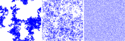
Figure 1: From left to right, the range in 2 dimensions, a slice in 3 dimensions and Bernoulli percolation, all of density 0.3.

Returning to our process, in Figure 1 simulation pictures are shown that give heuristical support to the view that although the range for $d\geq 3$ has long range dependence, it bears some similarities to i.i.d. site percolation. Indeed, one can see that the middle picture, a 2d slice of the range of a walk that filled 30% of a 3d torus, is “in between,” dependence-wise, the i.i.d. picture on the right and the highly dependent picture on the left where the effect of two-dimensional recurrence is evident. Thus, one might expect analogous geometric behavior of the range for $d\geq 3$ and i.i.d. percolation. This partially turns out to be the case.

In benjamini2008giant , the complement of the range, called the vacant set, is investigated by Benjamini and Sznitman. For positive $u$, it is shown $uN^{d}$ is indeed the proper timescale to generate percolative behavior of the vacant set. Starting at the uniform distribution, it is easily shown that for some $c(u,d)>0$, the probability a given vertex in the torus is visited by the walk is between $c$ and $1-c$, independently of $N$. A more difficult result is that for small $u$, the vacant set typically contains a connected component that is larger than some constant proportion of the torus. Indeed, simulations support the existence of a phase transition in $u$ of the vacant set geometry, where below some critical $u_{c}>0$, a unique giant component appears, and above it all clusters are microscopic.

The range, unlike the vacant set, does not display an obvious phase transition in $u$. It is connected for all positive $u$, and fills a $c^{\prime}(u,d)>0$ proportion of the torus with high probability. Despite the analogy to percolation being flawed in this respect, the range does display some percolative behavior due to the Markov property and uniform transience of a random walk in $d>2$. Roughly, conditioning on the vertices by which the walk enters and exits a small box makes the path in between them independent from the walk outside this box. Using this idea and facts from percolation theory gathered in Section 4, we prove the range does capture the distance and isoperimetric bounds of the torus, though our methods require an iterated logarithmic correction to the bounds of the full torus. In Section 6, it is shown that for arbitrarily small $u>0$, the range asymptotically dominates a recursive structure, defined in Section 2, which can roughly be described as a finite-level supercritical fractal percolation. From this structure, we extract distance bounds (Appendix B) and mixing bounds (Section 3) that are a $\log^{(k)}(N)=\log(\log(\cdots(\log(N)\cdots k\cdots)))$ factor from those on the torus.

Let us expand a bit on the heuristics presented in the previous paragraph. Since the holes in the range are larger than those in i.i.d. percolation (see the last comment in benjamini2008giant ), one can never hope to dominate it. Instead, we formulate a notion of density of a box of side $n$, which essentially means that it is crossed top to bottom (traversed) by the random walk an order of $n^{d-2}$ times. A union bound then gives that w.h.p. all $\log^{4}N$-sided “first-level” boxes in the torus possess this property. Next, given this condition, for each fixed first-level box, all internal “second-level” boxes of side $c\log^{4}(\log N)$ are dense w.h.p., and independently from other disjoint first-level boxes. The probability for the denseness of the second-level boxes is not high enough for a union bound on all of them, however, it is enough such that first-level boxes whose second-level boxes are all dense dominate $p$-percolation for arbitrarily high $p<1$. This is the basis of the hierarchical renormalization used below to prove the same fact for “$k$-level” boxes with arbitrary $k$. A drawback of this method is that the density of boxes becomes diluted by a constant factor from level to level, preventing us from continuing this rescaling to reach boxes of a bounded size. This dilution is the main source of the $\log^{(k)}(N)$ correction. We believe this correction is an artifact of the method and that the true bounds should be the same as those on the torus.

A central technical concept introduced in the paper is the recursively defined $k$-goodness of a box, which is roughly that the $(k-1)$-good smaller scale boxes inside satisfy some typical supercritical Percolation properties. The main demand from $0$-good boxes is that the range is connected in their interior. This provides a useful way to analyze the range but perhaps a better formulated notion will get sharper bounds. A second technique worth mentioning is the propagation of isoperimetric bounds through multiple scales in Lemma 3.3. This has been done for one level in mathieu2004isoperimetry , but it is not clear how to extend the method there to more than one level. Last, getting rid of dependence on time in the random walk when moving to smaller scale boxes is not trivial. To do this, we prove the domination of the $k$-good recursive structure mentioned above simultaneously for all $\{\mathcal{R}_{N}(t)\}_{t\geq uN^{d}}$, where $\mathcal{R}_{N}(t)$ is the range of the walk up to time $t$. This is facilitated by results on conditioned random walks from Section 5, in particular by Lemma 5.11. The lemma shows that given any fixed “boundary-connected-path” $f(t)$ in a dense box (see definition above Lemma 5.3), the random walk traversals will merge it w.h.p. into a single connected component, for all $t\geq 0$.

Using the results proved for the random walk on the torus, we prove a bound on the Heat kernal of random walk on Random Interlacements. In Appendix C, we write a short introduction on Random Interlacements where one can find the notation used in Section 7.

It should be mentioned that while all sections ahead require the terminology introduced in Section 2, all remaining sections apart from Section 6 may be read quite independently from one another. Section 6 also relies on random walk definitions from Section 5. For reading convenience, one can find an index of symbols in Appendix D.

2 Result and notation

Let $\mathcal{T}(N,d)$ be the discrete $d$-dimensional torus with side length $N$, for $d\geq 3$. Fixing $d$, $\mathcal{T}(V,E)$ is a graph with

$$V(N)=\bigl{\{}\mathbf{x}\in\mathbb{Z}^{d}\dvtx 0\leq x_{i}<N,1\leq i\leq d\bigr{\}}$$

and

$$E(N)=\bigl{\{}\{\mathbf{x},\mathbf{y}\}\subset V\bigl{(}\mathcal{T}(N)\bigr{)}\dvtx\Pi_{N}(\mathbf{x}-\mathbf{y})\in\{\pm\mathbf{e}_{1},\ldots,\pm\mathbf{e}_{d}\}\bigr{\}},$$

where $\Pi_{N}\dvtx\mathbb{Z}^{d}\to V(N)$ for $\mathbf{x}\in\mathbb{Z}^{d}$ is ${\Pi_{N}}(\mathbf{x})=(x_{1}\operatorname{mod}N,\ldots,x_{d}\operatorname{mod}N)$ and $\{\mathbf{e}_{i}\}_{i=1}^{d}$ is the standard basis of $\mathbb{Z}^{d}$.

Note that if $S(\cdot)$ is a simple random walk (SRW) in $\mathbb{Z}^{d}$, $S_{N}(\cdot)=\Pi_{N}\circ S(\cdot)$ is a SRW in $\mathcal{T}(N)$. Let $\mathcal{R}(t_{1},t_{2})=\{S(s)\dvtx t_{1}\leq s<t_{2}\}$ and call $\mathcal{R}(t)=\mathcal{R}(0,t)$ the range (until time $t$) of the walk. We consider $\mathcal{R}_{N}(t)$, the random connected subgraph of $\mathcal{T}$ induced by $\Pi_{N}\circ\mathcal{R}(t)$, where we include only edges traversed by the random walk. Throughout the paper, when no ambiguity is present, we identify a graph with its vertices.

Let $\mathbf{P}_{\mathbf{x}}[\cdot]$ be the law that makes $S(\cdot)$ an independent SRW starting at $\mathbf{x}\in\mathbb{Z}^{d}$. Below are the main three results of the paper.

Theorem 2.1

Set $u>0$ and for a graph $G$, let $d_{G}(\cdot,\cdot)$ denote graph distance. Then for any $k$,

$$\lim_{N\to\infty}\mathbf{P}_{\mathbf{0}}\biggl{[}\max_{t\geq uN^{d}}\biggl{\{}\frac{d_{\mathcal{R}_{N}(t)}(\mathbf{x},\mathbf{y})}{d_{\mathcal{T}(N)}(\mathbf{x},\mathbf{y})}\dvtx\mathbf{x},\mathbf{y}\in\mathcal{R}_{N}(t),d_{\mathcal{T}(N)}(\mathbf{x},\mathbf{y})>(\log N)^{5d}\biggr{\}}$$

$$\hskip 262.0pt{}>\log^{(k)}N\biggr{]}$$

$$\qquad=0,$$

where $\log^{(k)}N$ is $\log(\cdot)$ iterated $k$-times of $N$.

Since this paper was uploaded to the arXiv on 2010, the distance bounds where improved in cerny2011internal by Cernỳ and Popov. They managed to get a tight result without the $\log$ correction. Due to the improvement, the proof of Theorem 2.1 is postponed to Appendix B. Note that since distance bounds require finding one good path and isoperimetric bounds require a uniform bound on all subsets, the rest of the results in this paper do not follow the techniques of cerny2011internal .

Theorem 2.2

Set $u>0$ and let $\tau(G)$ be the (e.g., uniform) mixing time of a simple random walk on a graph $G$. Then for any $k$,

$$\lim_{N\to\infty}\mathbf{P}_{\mathbf{0}}\biggl{[}\max_{t\geq uN^{d}}\frac{\tau(\mathcal{R}_{N}(t))}{N^{2}}>\log^{(k)}N\biggr{]}=0.$$

The two theorems are a direct consequence of Theorem 6.1 and Theorems B.1, 3.1, respectively.

Using the same techniques for proving Theorem 2.1 and Theorem 2.2, we can show the next result for a random walk on the range of random interlacements (see Appendix C for notation).

Theorem 2.3

Let $u>0$ and $k\in{\mathbb{N}}$. Then there exists a constant $C(u,k)$ such that for $\mathbb{P}^{u}_{0}$ almost every ${\mathcal{I}}^{u}$, and for all $n$ large enough

$$\mathbf{P}_{0}^{u}[0,n]\leq\frac{C\cdot\log^{(k)}(n)}{n^{d/2}}.$$

This theorem quantifies the result of Ráth and Sapozhnikov in rath2011transience . Ráth and Sapozhnikov proved the graph of random interlacements is transient a.s.

The main purpose of the remainder of the section is to define a $k$-good configuration, and to establish notation used throughout the paper.

2.1 Graph notation

Given a graph $G$, we identify a subset of vertices $V$ with its induced subgraph in $G$. We denote $G\setminus V$, the complement of $V$ relative to $G$, by $V_{G}^{c}$. Writing $d_{G}(\cdot,\cdot)$ for the graph distance in $G$, we let $d_{G}(\mathbf{v},V)=\inf\{d_{G}(\mathbf{v},\mathbf{x})\dvtx\mathbf{x}\in V\}$. For the outer and inner boundary, we respectively write

$$\partial_{G}(V) = \bigl{\{}\mathbf{v}\in G\dvtx d_{G}(\mathbf{v},V)=1\bigr{\}},$$

$$\partial_{G}^{\mathrm{in}}(V) = \partial_{G}\bigl{(}V_{G}^{c}\bigr{)}=\bigl{\{}\mathbf{v}\in G\dvtx d\bigl{(}\mathbf{v},V_{G}^{c}\bigr{)}=1\bigr{\}}.$$

We often omit $G$ from the notation when the ambient graph is clear. We say $V$ is connected in $G$ if any two vertices in $V$ have a path in $G$ connecting them. $V_{1},V_{2}\subset G$ are connected in $G$ if $V_{1}\cup V_{2}$ is connected in $G$. Given $V\subset G$, we call a set that is connected in $V$ and is maximal to inclusion a component of $V$.

As noted above, we identify graphs and their vertices. Thus, $\mathbb{Z}^{d}$ denotes the $d$-dimensional integers as well as the graph on these vertices in which two vertices are connected if they differ by a unit vector.

Last, if $V\subset\mathbb{Z}^{d},\mathbf{z}\in\mathbb{Z}^{d}$ then $V\pm\mathbf{z}=\{\mathbf{x}\pm\mathbf{z}\dvtx\mathbf{x}\in V\}$.

2.2 Box notation

For $\mathbf{x}\in\mathbb{Z}^{d},n>0$, let

$$B(\mathbf{x},n)=\bigl{\{}\mathbf{y}\in\mathbb{Z}^{d}\dvtx\forall i,1\leq i\leq d,-n/2\leq\mathbf{x}(i)-\mathbf{y}(i)<n/2\bigr{\}}.$$

We write $B(n)$ if $\mathbf{x}$ is the origin, and when length and center are unambiguous we often just write $B$. Occasionally, we use lowercase $b$ for a smaller instance of a box. We denote the side length of a box by $\|B\|$, that is,

$$\|B\|=|B|^{{1}/{d}}.$$

Let $\operatorname{sp}\{B(\mathbf{x},n)\}=\{B(\mathbf{x}+\sum_{i}\mathbf{e}_{i}k_{i}n,n)\dvtx(k_{1},\ldots,k_{d})\in\mathbb{Z}^{d}\}$ where $\mathbf{e}_{1},\ldots,\mathbf{e}_{d}$ are the unit vectors in $\mathbb{Z}^{d}$, that is, all the nonintersecting translations of $B$ in $\mathbb{Z}^{d}$. We attach a graph structure to $\operatorname{sp}\{B(\mathbf{x},n)\}$ by defining the neighbors of a box $B(\mathbf{x},n)$ as $B(\mathbf{x}\pm\mathbf{e}_{i}n,n)$, $1\leq i\leq d$. Henceforth, any graph operators on a subset of some $\operatorname{sp}\{B\}$ refer to this graph structure. Observe that $\operatorname{sp}\{B(\mathbf{x},n)\}$ is isomorphic as a graph to $\mathbb{Z}^{d}$. We fix an isomorphism $\Delta\dvtx\operatorname{sp}\{B\}\to\mathbb{Z}^{d}$, $\Delta(B(\mathbf{x}+\sum_{i}\mathbf{e}_{i}k_{i}n,n))=\mathbf{x}+\sum_{i}\mathbf{e}_{i}k_{i}$. Using $\Delta$, we extend the definitions of a box to boxes as well. Thus, for a box $b=b(n)$ and an integer $m>0$, $B_{\Delta}(b,m)$ is a set of $m^{d}$ boxes. We use a big union symbol to denote internal union, that is, $\bigcup\mathbf{A}=\{\mathbf{x}\in A\dvtx A\in\mathbf{A}\}$. So in the preceding example, we have $\bigcup B_{\Delta}(b,m)=B(mn)$.

To ease the reading, we often refer to boxes that are neighbors under the above relationship as $\Delta$-neighbors, a connected set of boxes as $\Delta$-connected, and a component under $\Delta$-neighbor relationship a $\Delta$-component.

Definition 2.4.

Given a box $B(\mathbf{x},n)$, and $\alpha>0$, we write $B^{\alpha}$ for $B(\mathbf{x},\alpha n)$. Let

$$s(n)=\lceil\log n\rceil^{4}.$$

We write $s^{(i)}(n)$ to denote $s(\cdot)$ iterated $i$ times.

Definition 2.5.

Let

$$\sigma\bigl{(}B(\mathbf{x},n)\bigr{)}=\operatorname{sp}\bigl{\{}b\bigl{(}\mathbf{x},s(n)\bigr{)}\bigr{\}}\cap\bigl{\{}b\bigl{(}\mathbf{y},s(n)\bigr{)}\dvtx\mathbf{y}\in B\bigl{(}\mathbf{x},5n+3\lceil\log n\rceil^{6}\bigr{)}\bigr{\}}$$

be the subboxes of $B(\mathbf{x},n)$. Note that $B^{5}\subset\bigcup\sigma(B)$. $\sigma(B)$ is a collection of sub-boxes of side length $s(n)$ covering $B^{5}$; see Figure 2 for visualization.

We write $2^{A}$ for the power set of a set $A$, that is, the collection of subsets of $A$. We refer to finite subsets of $\mathbb{Z}^{d}$ as configurations.

Figure 2: $0$-good configuration.

2.3 Percolating configurations

Let $c_{a},c_{b}$ be fixed positive constants dependent only on dimension ($c_{a},c_{b}$ are determined in Lemma 4.8 and Corollary 4.6, resp.). $\omega\in 2^{B(n)}$ is a percolating configuration, denoted by ${\omega}\in{\mathcal{P}}(n)$, if there exists a subset which we call a good cluster $\mathcal{C}=\mathcal{C}(\omega)\subset\omega$, connected in $\omega$ (not necessarily maximal) for which the following properties hold: [1.]

$|\mathcal{C}|>(1-10^{-d})|B(n)|$.

The largest component in $B(n)\setminus\mathcal{C}$ is of size less than $(\log n)^{2}$.

For any $\mathbf{v},\mathbf{w}\in\mathcal{C}\cap B(n-c_{a}\log n)$ we have $d_{\mathcal{C}}(\mathbf{v},\mathbf{w})<c_{a}(d_{B}(\mathbf{v},\mathbf{w})\vee\log n)$. Moreover, a configuration $\omega\in{\mathcal{P}}(n)$ admits an isoperimetry property:

Let $T\subset B(n)$ satisfy $n^{1/5d}<|T|\leq n^{d}/2$, and assume both $T$ and $B(n)\setminus T$ are connected in $B(n)$. Then $|\partial_{B}T\cap\omega|,|\partial_{B}^{c}T\cap\omega|>c_{b}|T|^{(d-1)/d}$. The following claim is easy to check.

Claim 2.1

$\mathcal{P}(n)$ is a monotone set, that is, if $\omega\in\mathcal{P}(n)$ and $\omega\subset\omega^{+}\subset B(n)$ then $\omega^{+}\in\mathcal{P}(n)$.

2.4 $k$-good configurations

Let $c_{h}$ be a fixed positive constant dependent only on dimension ($c_{h}$ is determined in Theorem 5.12 below). For $n\in\mathbb{N},\rho>0$, and setting $B=B(n)$, a configuration $\omega\subset B^{7}$ belongs to $\mathcal{G}_{0}^{\rho}(n)$ if and only if the following properties hold: [1.]

For each $b\in\sigma(B)$, $|\omega\cap b|>(\rho c_{h}\wedge\frac{1}{2})|b|$.

For each $b\in\sigma(B)$, $\omega\cap b^{5}$ is connected in $\omega\cap b^{7}$.

Remark 2.6.

If $\omega\in\mathcal{G}_{0}^{\rho}(n)$, then for all $n>(\rho c_{h})^{-{1}/{d}}$: (i) $\omega$ intersects all $b\in\sigma(B)$ (property 1), and (ii) for any two $\Delta$-neighbors $b_{1},b_{2}\in\sigma(B)$, since $b_{2}\subset b_{1}^{5}$, $\omega\cap b_{1}$ and $\omega\cap b_{2}$ are connected in $\omega\cap b_{1}^{7}$ (property 2). In particular, $\omega\cap B^{5}$ is connected in $\omega\cap B^{7}$. See Figure 2 for a graphical explanation.

Let $\Lambda$ be a fixed positive constant dependent only on dimension ($\Lambda$ is determined in Theorem 5.8). For $k>0$, $\mathcal{G}_{k}^{\rho}(n)$ is defined recursively. Given $\omega\subset\mathbb{Z}^{d}$, $i\in{\mathbb{N}}$ and a box $b(\mathbf{x},m)$, we say $b$ is $(\omega,i,\rho)$-good if $(\omega\cap b^{7})-\mathbf{x}\in\mathcal{G}_{i}^{\rho}(m)$. Let

$$\mathcal{S}=\bigl{\{}b\in\sigma(B)\dvtx b\mbox{ is }(\omega,k-1,\rho\Lambda)\mbox{-good}\bigr{\}},$$

and let $\sigma_{B}=\|\Delta(\sigma(B))\|=|\sigma(B)|^{{1}/{d}}$. Then $\omega\in\mathcal{G}_{k}^{\rho}(n)$ if $\omega\in\mathcal{G}_{0}^{\rho}(n)$ and $\Delta(\mathcal{S})\in\mathcal{P}(\sigma_{B})$. See Figure 3 for a graphical explanation.

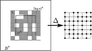
Figure 3: $k$-good configuration. All the grey subboxes are $k-1$-good, that is, ${\omega}\cap b\in{\mathcal{G}}_{k-1}^{\rho\Lambda}(\lceil\log n\rceil^{4})$. The configuration on the right is in ${\mathcal{P}}(\sigma_{B})$.

2.5 $k$-good torus

Let $\mathcal{T}=\mathcal{T}(N)$ and fix $\omega\subset\mathcal{T}$. Let $k\geq 0,\rho>0$. We define $(\omega,k,\rho)$-goodness of a torus. Let $n=\lceil N/10\rceil$. We call

$$\mathbf{T}=\operatorname{sp}\bigl{\{}B(n)\bigr{\}}\cap\bigl{\{}B(\mathbf{y},n)\dvtx\mathbf{y}\in B(N)\bigr{\}}$$

the top-level boxes for $\mathcal{T}$. Then $\mathcal{T}$ is a $(\omega,k,\rho)$-good torus if all boxes in $\mathbf{T}$ are $(\Pi_{N}^{-1}\omega,k,\rho)$-good.

Remark 2.6 therefore implies the following.

Remark 2.7.

If $\mathcal{T}(N)$ is a $(\omega,k,\rho)$-good torus, then $\omega$ is connected for all $N>C(\rho)$.

2.6 Constants

All constants are dependent on dimension by default and independent of any other parameter not appearing in their definition. Constants like $c,C$ may change their value from use to use. Numbered constants (e.g., $c_{1},C_{2}$) retain their value in a proof but no more than that, and constants tagged by a letter $(c_{a},c_{\Lambda})$ represent the same value throughout the paper.

3 Mixing bound

Given a finite connected graph $G$, let $X(t)$ be a lazy random walk on $G$. That is, denoting the walk’s transition matrix by $p(\cdot,\cdot)$, for any $\mathbf{v}\in G$ of degree $m$, $p(\mathbf{v},\mathbf{v})=1/2$ and $p(\mathbf{v},\mathbf{w})=1/2m$ for any neighbor $\mathbf{w}\in\partial\{\mathbf{v}\}$. We write $\tau(G)$ for the mixing time of $X(t)$ on $G$, that is,

$$\tau(G)=\min\biggl{\{}n\dvtx\biggl{|}\frac{p^{n}(x,y)-\pi(y)}{\pi(y)}\biggr{|}\leq\frac{1}{4},~{}\forall x,y\in V(G)\biggr{\}},$$

where $\pi$ is the stationary measure of the random walk on $G$. See morris2005evolving a thorough introduction on mixing times.

Theorem 3.1

Let $\omega_{0}\subset\mathcal{T}(N)$, $\rho>0$, $k\geq 1$. There is a $C(k,\rho)$ such that if $\mathcal{T}(N)$ is a $(\omega_{0},k,\rho)$-good torus then

$$\tau(\omega_{0})<CN^{2}\log^{(k-1)}N,$$

where $\log^{(m)}N$ is $\log(\cdot)$ iterated $m$ times of $N$.

We begin by stating and proving propositions required for Corollary 3.4, then using the corollary we prove Theorem 3.1.

Recall the definition of $\mathcal{G}_{l}^{\rho}(n)$ from Section 2.4. Let $c_{\rho}=(\rho c_{h}\wedge\frac{1}{2})/3$. We assume $n$ is large enough such that $\mathcal{G}_{l}^{\rho}(n)$ is nonempty, and that for any $\omega\in\mathcal{G}_{l}^{\rho}(n)$, $\omega\cap B^{5}(n)$ is connected in $\omega$ and satisfies $|\omega\cap B^{5}(n)|>3c_{\rho}n^{d}$ (see property 1 of $\mathcal{G}_{0}^{\rho}$ in Section 2.4 and Remark 2.6). In particular, there exists a set $S\subset\omega,|S\cap B^{5}(n)|\wedge|(\omega\setminus S)\cap B^{5}(n)|\geq c_{\rho}n^{d}$.

Since $\omega\cap B^{5}(n)$ is connected in $\omega$, we have the following.

Proposition 3.2

For any $l\geq 0$ and all large $n$, and $S\subset{\omega}\in\mathcal{G}_{l}^{\rho}(n)$

$$|\partial_{\omega}S|\geq 1.$$

Next, we bound $|\partial S|$ more accurately. The next theorem is one of the main results and techniques introduced in this paper. The theorem proves an almost tight isoperimetric inequality (up to an iterated $\log$). The main idea of the proof is induction on the number of iterations (which provide the iterated $\log$) and analyzing the geometry of renormalized subsets, that is, use the geometrical properties of the percolation configuration of good subboxes.

Theorem 3.3

Let $l\geq 0$, $\rho>0$, ${\omega}\in{\mathcal{G}}_{l}^{\rho}$ and $S\subset{\omega}$ such that $|S\cap B^{5}(n)|\wedge|(\omega\setminus S)\cap B^{5}(n)|=r\geq n^{{1}/{3}}$. There exists a constant $c_{1}(l,\rho)>0$, such that

$$|\partial_{\omega}S|>c_{1}(l,\rho)r^{{(d-1)}/{d}}\bigl{(}s^{(l)}(n)\bigr{)}^{1-d}.$$ (1)

The proof is by induction on $l$. For $l=0$, since $s^{(0)}(n)=n$, $|B^{5}(n)|^{{(d-1)}/{d}}s^{(0)}(n)^{1-d}$ is less than some $C_{1}$ for any $r\leq|B^{5}(n)|$. Thus, the base case of $l=0$ is given in Proposition 3.2 and the connectedness of ${\omega}$ with $c_{1}(0)=C_{1}^{-1}$. Now fix $l>0,\rho>0$ and assume (1) is true for $l-1$ with constant $c_{1}(l-1,\rho\Lambda)>0$, for all large $n$ and $n^{1/3}\leq r\leq|B^{5}(n)|$.

Our default ambient graph for $S$ is $\omega$. Thus, for $S\subset\omega$, $S^{c}=\omega\setminus S$ and $\partial S=\partial_{\omega}S$. Note that as $|S|\geq r$, if $|\partial S|>|S|^{(d-1)/d}$ we are done. W.l.o.g. assume $|S^{c}\cap B^{5}|\geq|S\cap B^{5}|$ since $|\partial_{\omega}S^{c}|\sim|\partial_{\omega}S|$.

Let $B=B(n)$ and let $m=s(n)$. For $0<\alpha<1$, let

$$\mathbf{F}=\mathbf{F}(\omega,S,\alpha)=\bigl{\{}b\in\sigma(B)\dvtx|b\cap S|\geq\alpha|b\cap\omega|\bigr{\}},$$

be the $\alpha$-filled subboxes. By the pigeon hole principle, there are ${\alpha}(\rho)<1$, $c_{2}(\rho)>0$, such that

$$|\mathbf{F}|<(1-c_{2})\bigl{|}\sigma(B)\bigr{|}.$$ (2)

Let $\mathbf{T}=\mathbf{T}(\omega,S)=\{b\in\sigma(B)\dvtx b\cap S\neq\varnothing\}$, then $|\mathbf{T}|\geq|S|m^{-d}$. The proof is separated into cases depending on the size of $F$. We begin with the case that $|\mathbf{F}|$ is small.

If $|\mathbf{F}|\leq\frac{1}{2}|S|m^{-d}$ then by the trivial lower bound on $\mathbf{T}$, $|\mathbf{T}\setminus\mathbf{F}|\geq\frac{1}{2}|S|m^{-d}$. For any box $b\in\mathbf{T}\setminus\mathbf{F}$, we have $\mathbf{x},\mathbf{y}\in b$ such that $\mathbf{x}\in S,\mathbf{y}\in S^{c}$. Since $\mathbf{x},\mathbf{y}$ are connected in $\omega\cap b^{7}$ (property 2 of $\mathcal{G}_{0}^{\rho}$), $\partial S\cap b^{7}\neq\varnothing$. For any box $b\in\sigma(B)$, there are at most $50d$ boxes $b^{\prime}\in\sigma(B)$ such that $b^{7}\cap b^{\prime 7}\neq\phi$. Since $|S|\geq n^{1/3}$ and $m^{d}$ is $o(n^{1/4d})$ we have for all large $n$,

$$|\partial S|\geq\frac{1}{50d}|\mathbf{T}\setminus\mathbf{F}|\geq\frac{1}{100d}|S|m^{-d}>|S|^{1-{3}/{(4d)}}>|S|^{{(d-1)}/{d}},$$

and are done with this case.

Our default ambient graph for sets of subboxes is $\sigma(B)$ with the box ($\Delta$) neighbor relationship (see Section 2.2). Thus, for $\mathbf{A}\subset\sigma(B)$, $\mathbf{A}^{c}=\sigma(B)\setminus\mathbf{A}$, $\partial\mathbf{A}=\partial_{\sigma(B)}\mathbf{A}$, $\partial^{\mathrm{in}}\mathbf{A}=\partial_{\sigma(B)}^{\mathrm{in}}\mathbf{A}$. We introduce edge boundary notation

$$\partial^{e}(\mathbf{Q})=\bigl{\{}\bigl{\{}b,b^{\prime}\bigr{\}}\dvtx b\sim b^{\prime},b\in\mathbf{Q},b^{\prime}\in\mathbf{Q}^{c}\bigr{\}}.$$

In the case that remains, $|\mathbf{F}|>\frac{1}{2}|S|m^{-d}$. Note that any box $b\in\partial\mathbf{F}$ satisfies $|b^{5}\cap S|\wedge|b^{5}\cap S^{c}|>c^{\prime}(\rho)m^{d}$. Hence, if we knew that $\mathbf{F}$ was a single $\Delta$-connected component with a connected complement, we could lower bound $|\partial\mathbf{F}|$ and use the fact that $\partial\mathbf{F}$ is a typical set (Percolation property 4) to get that a constant proportion of $\partial\mathbf{F}$ are $(\omega,l-1,\rho\Lambda)$-good boxes. Together with our induction hypothesis, this would complete the proof.

$$|\partial S| \geq \bigl{|}\partial S\cap\partial\mathbf{F}\cap_{b\in{\mathcal{G}}_{l-1}^{{\lambda}\rho}(m)}\{b\}\bigr{|}\geq c|\partial\mathbf{F}|m^{d-1}\bigl{(}s^{l-1}(m)\bigr{)}^{1-d}$$

$$\geq c|\mathbf{F}|^{{(d-1)}/{d}}m^{d-1}\bigl{(}s^{l}(n)\bigr{)}^{1-d}\geq\frac{c}{2}|S|^{{(d-1)}/{d}}m^{1-d}m^{d-1}\bigl{(}s^{l-1}(m)\bigr{)}^{1-d}$$

$$= \frac{c}{2}|S|^{{(d-1)}/{d}}\bigl{(}s^{l-1}(m)\bigr{)}^{1-d}.$$

$\mathbf{F}$ is not in general so nice. However, being of size greater than $\frac{1}{2}|S|m^{-d}$ implies there is a $c_{3}(\rho)>0$ and a set $\mathbb{K}=\mathbb{K}(\mathbf{F})\subset 2^{\sigma(B)}$ with the following properties for all large $n$, allowing us to make a similar isoperimetric statement:

$$\displaystyle\sum_{\mathbf{f}\in\mathbb{K}}\bigl{(}|\mathbf{f}|\wedge\bigl{|}\mathbf{f}^{c}\bigr{|}\bigr{)}\geq c_{3}|S|m^{-d},$$ (4)

$$\forall\mathbf{f}\in\mathbb{K},\qquad\partial\mathbf{f}\subset\mathbf{F}^{c},\qquad\partial^{\mathrm{in}}\mathbf{f}\subset\mathbf{F},$$ (5)

$$\forall\mathbf{f}_{1},\mathbf{f}_{2}\in\mathbb{K},\qquad\mathbf{f}_{1}\neq\mathbf{f}_{2}\quad\Longrightarrow\quad\partial^{e}\mathbf{f}_{1}\cap\partial^{e}\mathbf{f}_{2}=\varnothing,$$ (6)

$$\forall\mathbf{f}\in\mathbb{K},\qquad\mathbf{f},\mathbf{f}^{c}\mbox{ are }\Delta\mbox{-connected},$$ (7)

$$n^{1/5d}<|\mathbf{f}|\wedge\bigl{|}\mathbf{f}^{c}\bigr{|}\leq\bigl{|}\sigma(B)\bigr{|}/2.$$ (8)

First, we show how the proof follows from the existence of $\mathbb{K}$. Let $\mathbf{G}=\mathbf{G}(\omega,l,\rho)$ be the set of $(\omega,l-1,\rho\Lambda)$-good subboxes in $\sigma(B)$. By (7), (8) and Percolation property 4 (see Section 2.3), for all large enough $n$, for any $\mathbf{f}\in\mathbb{K}$, $|\partial\mathbf{f}\cap\mathbf{G}|>c_{b}(|\mathbf{f}|\wedge|\mathbf{f}^{c}|)^{(d-1)/d}$. Let $\mathbb{K}^{\partial}=\{\partial\mathbf{f}\dvtx\mathbf{f}\in\mathbb{K}\}$. By (6), for any $b\in\sigma(B)$, $|\{\mathbf{f}\in\mathbb{K}^{\partial}\dvtx b\in\mathbf{f}\}|\leq 2d$. Thus,

$$\Bigl{|}\bigcup\mathbb{K}^{\partial}\cap\mathbf{G}\Bigr{|}\geq\frac{1}{2d}\sum_{\mathbf{f}\in\mathbb{K}}c_{b}\bigl{(}|\mathbf{f}|\wedge\bigl{|}\mathbf{f}^{c}\bigr{|}\bigr{)}^{(d-1)/d}.$$

By subadditivity of $x^{\beta}$ where $\beta<1$ and (4) this gives

$$\Bigl{|}\bigcup\mathbb{K}^{\partial}\cap\mathbf{G}\Bigr{|}\geq c\biggl{[}\sum_{\mathbf{f}\in\mathbb{K}}\bigl{(}|\mathbf{f}|\wedge\bigl{|}\mathbf{f}^{c}\bigr{|}\bigr{)}\biggr{]}^{(d-1)/d}\geq c^{\prime}\frac{|S|^{(d-1)/d}}{m^{d-1}}.$$ (9)

Let $\mathbf{A}\subset\bigcup\mathbb{K}^{\partial}\cap\mathbf{G}$, be a subset of size $|A|>c|\bigcup\mathbb{K}^{\partial}\cap\mathbf{G}|$, satisfying that for any distinct $b_{1},b_{2}\in\mathbf{A}$, $b_{1}^{7}\cap b_{2}^{7}=\varnothing$, for example, $A=(\bigcup\mathbb{K}^{\partial}\cap\mathbf{G})\cap\Delta^{-1}(20\cdot\mathbb{Z}^{d})$. By (5), for any $b\in\mathbf{A}$, $b\in\mathbf{F}^{c}$ but has a $\Delta$-neighbor $b^{\prime}\in\mathbf{F}$, implying $|S\cap b^{5}|\wedge|S^{c}\cap b^{5}|\geq c(\hat{\alpha},\rho)m^{d}=\hat{c}m^{d}$. Since $\mathbf{A}\subset\mathbf{G}$, using our induction assumption and that $|S|>r$,

$$|\partial S| \geq \Bigl{|}\partial S\cap\bigcup\mathbf{F}\Bigr{|}\stackrel{{\scriptstyle\scriptsize{(\ref{eqedgeoffexactlyoneisfilled})}}}{{\geq}}|\partial S\cap A|\stackrel{{\scriptstyle\scriptsize{(\ref{eqksize})}}}{{\geq}}c^{\prime}\frac{|S|^{(d-1)/d}}{m^{d-1}}m^{d-1}\bigl{(}s^{l-1}(m)\bigr{)}^{1-d}$$

$$= c^{\prime}|S|^{{(d-1)}/{d}}\bigl{(}s^{l}(n)\bigr{)}^{1-d}$$

and we are done.

We return to proving the existence of $\mathbb{K}$.

Recall, a $\Delta$-component of a set $\mathbf{Q}\subset\sigma(B)$ is a maximal connected component in $\mathbf{Q}$ according to the box neighbor relationship (see Section 2.2). Let $\mathbb{F}$ be the set of $\Delta$-components of $\mathbf{F}$. Since $\mathbf{F}\neq\sigma(B)$, for any $\mathbf{f}\in\mathbb{F}$, there exists $b\in\mathbf{f}$ with a $\Delta$-neighbor $b^{\prime}\in\mathbf{f}^{c}$, such that $b^{\prime}\subset b^{5}$. As before, by property 2 of $\mathcal{G}_{0}^{\rho}$ (see Section 2.4), $b^{7}\cap\partial S\neq\varnothing$. Letting $\mathbf{F}^{\partial}=\{b\in\mathbf{F}\dvtx b^{7}\cap\partial S\neq\varnothing\}$, we then have $|\mathbf{F}^{\partial}|\geq|\mathbb{F}|$. Since we can extract a subset $\mathbf{A}\subset\mathbf{F}^{\partial}$ where $|\mathbf{A}|>c|\mathbf{F}^{\partial}|$, and for any distinct $b_{1},b_{2}\in\mathbf{A}$, $b_{1}^{7}\cap b_{2}^{7}=\varnothing$, we only need deal with the case $|\mathbb{F}|<|S|^{1-{1}/{(2d)}}$. Let $\mathbb{H}$ be the set of $\Delta$-components of $\mathbf{F}^{c}$. In the same way, we may assume $|\mathbb{H}|<|S|^{1-{1}/{(2d)}}$. By (2), $|\mathbf{F}^{c}|>c_{2}|\sigma(B)|>2c_{3}|S|m^{-d}$. We also assumed $|\mathbf{F}|>\frac{1}{2}|S|m^{-d}$, so w.l.o.g. $c_{3}<1/4$ and

$$\bigl{|}\mathbf{F}^{c}\bigr{|},|\mathbf{F}|>2c_{3}|S|m^{-d}.$$ (11)

Let $\widehat{\mathbb{F}}=\{\mathbf{f}\in\mathbb{F}\dvtx|\mathbf{f}|\geq c_{3}|S|^{{1}/{(2d)}}m^{-d}\}$ and let $\widehat{\mathbb{H}}=\{\mathbf{h}\in\mathbb{H}\dvtx|\mathbf{h}|\geq\break c_{3}|S|^{{1}/{(2d)}}m^{-d}\}$. We assumed $|\mathbb{F}|,|\mathbb{H}|<|S|^{1-{1}/{(2d)}}$, and thus $\bigcup(\mathbb{F}\setminus\widehat{\mathbb{F}}),\bigcup(\mathbb{H}\setminus\widehat{\mathbb{H}})<c_{3}|S|m^{-d}$. So, from (11), we get

$$\Bigl{|}\bigcup\widehat{\mathbb{F}}\Bigr{|},\Bigl{|}\bigcup\widehat{\mathbb{H}}\Bigr{|}>c_{3}|S|m^{-d}.$$ (12)

Let

$$\mathbb{K}=\bigl{\{}\mathbf{f}\subset\sigma(B)\dvtx\mathbf{f}\mbox{ is a }\Delta\mbox{-component of }\mathbf{h}^{c},\mathbf{h}\in\mathbb{H},|\mathbf{f}|\wedge\bigl{|}\mathbf{f}^{c}\bigr{|}>c_{3}|S|^{{1}/{(2d)}}m^{-d}\bigr{\}}.$$

Let $U\dvtx\mathbb{K}\to\mathbb{H}$ where for $\mathbf{f}\in\mathbb{K}$, $U(\mathbf{f})$ is the unique element in $\mathbb{H}$ for which $\mathbf{f}$ is a $\Delta$-component of $U(\mathbf{f})^{c}$. For each $\mathbf{f}\in\mathbb{K}$, $\partial\mathbf{f}\subset U(\mathbf{f})\subset\mathbf{F}^{c}$ and because $U(\mathbf{f})$ is a component of $\mathbf{F}^{c}$, $\partial^{\mathrm{in}}\mathbf{f}\subset\mathbf{F}$, giving us (5). Let $\mathbf{h}\in\widehat{\mathbb{H}}$. For any $\mathbf{f}\in\widehat{\mathbb{F}}$, $\mathbf{f}\subset\mathbf{h}^{c}$ and thus $\mathbf{f}$ is contained in some $\Delta$-component of $\mathbf{h}^{c}$ which we denote $\hat{\mathbf{f}}$. Since $\mathbf{h}\subset\hat{\mathbf{f}}^{c}$ and $\mathbf{f}\subset\hat{\mathbf{f}}$ we get $\hat{\mathbf{f}}\in\mathbb{K}$ and in particular, $\hat{\mathbf{f}}\in U^{-1}(\mathbf{h})$. Thus, for any $\mathbf{h}\in\widehat{\mathbb{H}}$, $\bigcup\widehat{\mathbb{F}}\subset\bigcup U^{-1}(\mathbf{h})$. In Figure 4, we give an example of some $\mathbf{F}$ and the resulting $\mathbb{K}$.

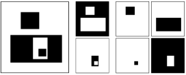
Figure 4: Example of $\mathbf{F}$ and resulting $\mathbb{K}=\{\mathbf{f}_{1},\mathbf{f}_{2},\mathbf{f}_{3},\mathbf{f}_{4}\}$. $\left[\mathbf{F}\hskip 4.0pt{\mathbf{h}_{1}\enskip\mathbf{f}_{1}\enskip\mathbf{f}_{2}\atop\mathbf{h}_{2}\enskip\mathbf{f}_{3}\enskip\mathbf{f}_{4}}\right]$ where the sets are in black and $\mathbf{h}_{1}=U(\mathbf{f}_{1})=U(\mathbf{f}_{2})$, $\mathbf{h}_{2}=U(\mathbf{f}_{3})=U(\mathbf{f}_{4})$.

We regroup terms in the sum and use the fact that for any $\mathbf{h}\in\mathbb{H},\mathbf{f}\in U^{-1}(\mathbf{h})$, we have $\mathbf{h}\subset\mathbf{f}^{c}$ to get:

$$\sum_{\mathbf{f}\in\mathbb{K}}\bigl{(}|\mathbf{f}|\wedge\bigl{|}\mathbf{f}^{c}\bigr{|}\bigr{)}\geq\sum_{\mathbf{h}\in\widehat{\mathbb{H}}}\sum_{\mathbf{f}\in U^{-1}(\mathbf{h})}\bigl{(}|\mathbf{f}|\wedge\bigl{|}\mathbf{f}^{c}\bigr{|}\bigr{)}\geq\sum_{\mathbf{h}\in\widehat{\mathbb{H}}}\sum_{\mathbf{f}\in U^{-1}(\mathbf{h})}\bigl{(}|\mathbf{f}|\wedge|\mathbf{h}|\bigr{)}.$$

If there exists $\mathbf{h}^{*}\in\widehat{\mathbb{H}}$ such that for any $f\in U^{-1}(\mathbf{h}^{*})$, $|\mathbf{h}^{*}|\geq|\mathbf{f}|$, we have

$$\sum_{\mathbf{f}\in\mathbb{K}}\bigl{(}|\mathbf{f}|\wedge\bigl{|}\mathbf{f}^{c}\bigr{|}\bigr{)}\geq\sum_{\mathbf{f}\in U^{-1}(\mathbf{h}^{*})}|\mathbf{f}|=\Bigl{|}\bigcup U^{-1}\bigl{(}\mathbf{h}^{*}\bigr{)}\Bigr{|}\geq\Bigl{|}\bigcup\widehat{\mathbb{F}}\Bigr{|}.$$

If none such exists, then

$$\sum_{\mathbf{f}\in\mathbb{K}}\bigl{(}|\mathbf{f}|\wedge\bigl{|}\mathbf{f}^{c}\bigr{|}\bigr{)}\geq\sum_{\mathbf{h}\in\widehat{\mathbb{H}}}|\mathbf{h}|=\Bigl{|}\bigcup\widehat{\mathbb{H}}\Bigr{|}.$$

Thus, from (12), we get (4). Next, for $\mathbf{f}_{1}\in\mathbb{K}$, any edge $\{b,\hat{b}\}\in\partial^{e}\mathbf{f}_{1}$ satisfies w.l.o.g. $\hat{b}\in U(\mathbf{f}_{1})$ and $b\in\mathbf{f}_{1}$. Thus, if $\mathbf{f}_{2}\in\mathbb{K}$ shares the edge $\{b,\hat{b}\}$ with $\mathbf{f}_{1}$, then $U(\mathbf{f}_{1})=U(\mathbf{f}_{2})$ and since $b\in\mathbf{f}_{1}\cap\mathbf{f}_{2}$ and both are $\Delta$-components of $U(\mathbf{f}_{1})^{c}$, we have $\mathbf{f}_{1}=\mathbf{f}_{2}$, giving us (6). To get (7), let $\mathbf{h}\in\mathbb{H}$, and let $\mathbf{h}^{c}=\mathbf{f}_{1}\cup\cdots\cup\mathbf{f}_{n}$ where $\mathbf{f}_{i}$ are the $\Delta$-components of $\mathbf{h}^{c}$. Then $\forall i,\partial\mathbf{f}_{i}\subset\mathbf{h}$, and since $\mathbf{h}$ is connected, $\mathbf{f}_{i},\mathbf{f}_{j}$ are connected in $\mathbf{f}_{i}\cup\mathbf{f}_{j}\cup\mathbf{h}$ for any $i,j$. This implies $\mathbf{f}_{i}^{c}=\mathbf{h}\cup\mathbf{f}_{1}\cup\cdots\cup\mathbf{f}_{n}\setminus\mathbf{f}_{i}$ is $\Delta$-connected for any $i$. Last, since $|\mathbf{f}|\wedge|\mathbf{f}^{c}|>c_{3}|S|^{{1}/{(2d)}}m^{-d}$ and $m^{d}$ is $o(n^{1/20d)}$, we get (8). In the below corollary, we transfer the isoperimetric bounds on $\varphi$ from the setting of a box to a torus. The main idea of the proof is to show that given any large set $S$ in a $(\omega,k,\rho)$-good torus, there are two neighboring top-level boxes which have a large intersection with $S$ and $\omega\setminus S$.

Corollary 3.4

Let $\omega\subset\mathcal{T}(N)$. If $\mathcal{T}(N)$ is a $(\omega,k,\rho)$-good torus then for all large enough $N$, and $r\geq N$

$$\hat{\phi}(r) = \inf\biggl{\{}\frac{|\partial_{\omega}S|}{|S|}\dvtx S\subset\omega,N^{{1}/{3}}\leq|S|\leq r\wedge\biggl{(}1-\frac{1}{4d}\biggr{)}|\omega|\biggr{\}}$$

$$> c(k,\rho)\frac{r^{-1/d}}{(s^{(k)}(N))^{d-1}}.$$

Let $\omega^{+}=\Pi_{N}^{-1}(\omega)\cap B^{3}(N)$. Recall from Section 2.5 that all top-level boxes for $\mathcal{T}(N)$ are $(\omega^{+},k,\rho)$-good, so by property 1 of $\mathcal{G}_{0}^{\rho}$, for any top-level box $B$, there is a $c_{1}(\rho)>0$ such that

$$\bigl{|}B\cap\omega^{+}\bigr{|}>c_{1}N^{d}.$$ (13)

Fix $r\geq N$. By construction, $\frac{1}{2d}|\omega^{+}|=|\omega|\geq|B\cap\omega^{+}|$ for any top-level box $B$. We assume that $N$ is large enough so that $c_{1}N^{d-1}>4d$, and $|B\cap\omega^{+}|>4\,dN$. In particular, this implies that the infimum is not on an empty set. Let $S$ satisfy the conditions to be a candidate for the infimum in $\hat{\phi}(r)$ and extend it to $S^{+}=\Pi_{N}^{-1}(S)\cap B^{3}(N)$. Let $\hat{r}=|S|\wedge|\omega\setminus S|$. Again by (13), for each top-level box $B$, $|B\cap S^{+}|\vee|B\cap(\omega^{+}\setminus S^{+})|\geq\frac{1}{2}c_{1}N^{d}>c_{2}\hat{r}$. On the other hand, since there are $10^{d}$ top-level boxes whose union covers $B(N)$, by the pigeonhole principle, there must be some box $B$ for which $|B\cap S^{+}|\geq 10^{-d}|S|$ and likewise a box $B^{\prime}$ for which $|B^{\prime}\cap(\omega^{+}\setminus S^{+})|\geq 10^{-d}|(\omega\setminus S)|$. Let $c_{3}=c_{2}\wedge 10^{-d}$. Since the top-level boxes are $\Delta$-connected, there are two $\Delta$-neighboring top-level boxes $B_{1},B_{2}$ such that $|B_{1}\cap S^{+}|,|B_{2}\cap(\omega^{+}\setminus S^{+})|\geq c_{3}\hat{r}$. This implies $|B_{1}^{5}\cap S^{+}|\wedge|B_{1}^{5}\cap(\omega^{+}\setminus S^{+})|\geq c_{3}\hat{r}$. By construction, $|\partial_{B_{1}^{7}\cap\omega^{+}}S^{+}|\leq|\partial_{\omega}S|$. Since $B_{1}$ is $(\omega^{+},k,\rho)$-good, we can use Theorem 3.3 to lower bound $|\partial_{B_{1}^{7}\cap\omega^{+}}S^{+}|$ by $c\hat{r}^{{(d-1)}/{d}}(s^{(k)}(N))^{1-d}$ for all large $N$. Note that as $|\omega|>4\,dN$, implying $|\omega\setminus S|\geq N$, we have $\hat{r}\geq N$. Since $|\omega\setminus S|\geq\frac{1}{4d}|\omega|>\frac{1}{4d}|S|$, we can bound $|S|$, the denominator in the infimum, from above by $4d\hat{r}$, giving us $\frac{|\partial_{\omega}S|}{|S|}\geq c\hat{r}^{-1/d}(s^{(k)}(N))^{1-d}$. Since $\hat{r}\leq r$ we are done. We now proceed to prove the main theorem of this section. Proof of Theorem 3.1 The following proof makes assumptions which are valid for all but a finite number of $N$, and those are resolved by the large constant above. Note that $\omega_{0}$ is viewed as a subgraph of $\mathcal{T}(N)$ as far as connectivity is concerned. We present an upper bound to the mixing time $\tau$ of $X(t)$ using average conductance, a method developed in lovasz1999faster and refined in subsequent papers.

We follow notation of morris2005evolving . Let $\pi(\cdot)$ be the stationary distribution of $X(t)$ and for $\mathbf{x},\mathbf{y}\in\omega_{0}$ let $Q(\mathbf{x},\mathbf{y})=\pi(\mathbf{x})p(\mathbf{x},\mathbf{y})$. For $S,A\subset\omega_{0}$ let $Q(S,A)=\sum_{\mathbf{s}\in S,\mathbf{a}\in A}Q(\mathbf{s},\mathbf{a})$. Let $\Phi_{S}=\frac{Q(S,S^{c})}{\pi(S)}$ and let $\Phi(u)=\inf\{\Phi_{S}\dvtx 0<\pi(S)\leq u\wedge\frac{1}{2}\}$. Let $\pi_{*}=\min_{\mathbf{x}\in\omega_{0}}\pi(\mathbf{x})$.

By morris2005evolving ,

$$\tau=\tau\biggl{(}\omega_{0},\frac{1}{4}\biggr{)}\leq 1+\int_{4\pi_{*}}^{16}\frac{4\,du}{u\Phi^{2}(u)}.$$ (14)

Recall the notation from Section 2.1. In this proof, our ambient graph is $\omega_{0}$ and thus $S^{c}=\omega_{0}\setminus S$ and $\partial S=\partial_{\omega_{0}}S$. To simplify notation in the proof, we restate (14) in terms of internal volume and boundary size.

For $S\subset\omega_{0}$, if $\pi(S)\leq u$, then we have by definition $u\geq\sum_{\mathbf{v}\in S}\deg(\mathbf{v})\times[\sum_{\mathbf{v}\in\omega_{0}}\deg(\mathbf{v})]^{-1}$. Using the bound on degree and connectedness of ${\omega}_{0}$, we get $|S|\leq 2ud|\omega_{0}|$. In the same way, $2d\frac{|S^{c}|}{|\omega_{0}|}>\pi(S^{c})\geq 1-u$ which gives $|S|\leq(1-\frac{1}{2d}(1-u))|\omega_{0}|$, and thus for $u\leq\frac{1}{2}$,

$$|S|\leq 2ud|\omega_{0}|\wedge\biggl{(}1-\frac{1}{4d}\biggr{)}|\omega_{0}|.$$ (15)

Let $\phi_{S}=\frac{|\partial S|}{|S|}$. Since $\omega_{0}$ is a bounded degree graph and $\mathbf{x}\sim\mathbf{y}\iff\frac{1}{4d}\leq p(\mathbf{x},\mathbf{y})\leq\frac{1}{2}$, for some $C(d)$ and all $S\subset\omega_{0}$ we have $\phi_{S}<C\Phi_{S}$. Let $\phi(r)=\inf\{\phi_{S}\dvtx 0<|S|\leq r\wedge(1-\frac{1}{4d})|\omega_{0}|\}$. Then by (15) the infimum in $\phi(2ud|\omega_{0}|)$ is on a larger set than the infimum in $\Phi(u)$ giving us $\phi(2ud|\omega_{0}|)<C\Phi(u)$. Thus, by the change of variables $r=2ud|\omega_{0}|$ in (14), we get

$$\tau<C\int_{1}^{32dN^{d}}\frac{dr}{r\phi^{2}(r)}.$$ (16)

We continue by showing that for our purposes, a rough estimate of $\phi_{S}$ for sufficiently small sets $S$ is enough. Let

$$\hat{\phi}(r)=\inf\biggl{\{}\phi_{S}\dvtx N^{{1}/{3}}\leq|S|\leq r\wedge\biggl{(}1-\frac{1}{4d}\biggr{)}|\omega_{0}|\biggr{\}},$$

where the infimum of an empty set is $\infty$. Since $\omega_{0}$ is connected (see Remark 2.7), $\phi(r)\geq 1/r$ for any $1\leq r<|\omega_{0}|$. For large $N$, by property 1 of $\mathcal{G}_{0}^{\rho}$ (see Section 2.4), $N<(1-\frac{1}{4d})|\omega_{0}|$. Thus,

$$\phi(r) = \inf\bigl{\{}\phi_{S}\dvtx|S|\leq r\wedge N^{{1}/{3}}\bigr{\}}\wedge\hat{\phi}(r)$$

$$\geq \bigl{[}r^{-1}\vee N^{-{1}/{3}}\bigr{]}\wedge\hat{\phi}(r).$$

By Corollary 3.4 below, $\hat{\phi}(r)>c(k,\rho)(s^{(k)}(N))^{1-d}r^{-1/d}$. Integrating (16) with the above lower bound for $\phi(r)$, we thus get

$$\tau < C\int_{1}^{32N^{d}}\frac{dr}{r(N^{-{1}/{3}})^{2}}+C\int_{10^{d}N^{{1}/{3}}}^{32N^{d}}\frac{dr}{r\hat{\phi}^{2}(r)}$$

$$< o\bigl{(}N^{2}\bigr{)}+C\bigl{(}s^{(k)}(N)\bigr{)}^{2d-2}N^{2}=o\bigl{(}\bigl{(}\log^{(k-1)}N\bigr{)}\bigr{)}N^{2}$$

as required.

4 High density percolation percolates

This section presents results used in the renormalization arguments of Section 6. See Section 2.3 for the properties of percolating configuration. Note that many of the lemmas in this section deal with i.i.d. Bernoulli percolation.

Lemma 4.1

For $n\in\mathbb{N}$, let $\{Y(\mathbf{z})\}_{\mathbf{z}\in B(n)}$ be i.i.d. $\{0,1\}$ r.v.’s, and write $\mathcal{S}(n)=\{\mathbf{z}\in B(n)\dvtx Y(\mathbf{z})=1\}$ for the random support of $Y$. Then there are dimensional dependent constants, $C>0$ and $p_{b}<1$, such that if $\Pr[Y(\mathbf{0})=1]=p_{b}$,

$$\Pr\bigl{[}\mathcal{S}(n)\in\mathcal{P}(n)\bigr{]}\geq 1-\frac{C(\log n)^{d-1}}{n^{d}}.$$

Lemmas 4.3, 4.7, 4.8 and Corollary 4.6 prove Percolation properties 1–4, respectively. The next lemma assures a percolation configuration given a finite range dependance requirement.

Corollary 4.2

For $n\in\mathbb{N}$, let $\{Y(\mathbf{z})\}_{\mathbf{z}\in B(n)}$ be $\{0,1\}$ r.v.’s, not necessarily i.i.d., and write $\mathcal{S}(n)=\{\mathbf{z}\in B(n)\dvtx Y(\mathbf{z})=1\}$ for the random support of $Y$. Assume the r.v.’s have the property that for any $\mathbf{x}\in B(n)$ and any $A\subset B(n)\setminus b(\mathbf{x},20)$,

$$\Pr\bigl{[}Y(\mathbf{x})=1|\mathcal{S}\cap B(n)\setminus b(\mathbf{x},20)=A\bigr{]}>p_{d},$$

where $p_{d}<1$ is a fixed constant dependent only on $p_{b}$ (from Lemma 4.1) and dimension.

Then for all $p<1$, there is a $C(p)<\infty$ such that for all $n>C$,

$$\Pr\bigl{[}\mathcal{S}(n)\in\mathcal{P}(n)\bigr{]}>p.$$

The domination of product measures result of Liggett, Schonmann and Stacey liggett1997domination , implies there is a $p_{d}<1$ for which $\mathcal{S}(n)$ stochastically dominates an i.i.d. product field with density $p_{b}$ on $B(n)$. Lemma 4.1 tells us that the probability such an i.i.d. field belongs to $\mathcal{P}(n)$ approaches one as $n$ tends to infinity. Since Percolation properties are monotone (Claim 2.1), we are done. Write $\mathbf{P}_{p}[\cdot]$ for the law that makes $\{Y(\mathbf{z})\}_{\mathbf{z}\in\mathbb{Z}^{d}}$ i.i.d. $\{0,1\}$ r.v.’s where $Y(\mathbf{z})=1$ w.p. $p$. Let $B=B(n)$ and write $\mathcal{S}=Y^{-1}(1)\cap B$ for the random set of open sites in $B$. Denote by $\mathcal{C}$ the largest connected component in $\mathcal{S}$.

We write a consequence of Theorem 1.1 of deuschel1996surface . One can find the proof in the appendix of procaccia2011concentration .

Lemma 4.3

There is a $p_{0}(d)<1$ such that for every $p>p_{0}$, there exists a $c>0$ such that

$$\mathbf{P}_{p}\bigl{[}|\mathcal{C}|<\bigl{(}1-10^{-d}\bigr{)}\bigl{|}B(n)\bigr{|}\bigr{]}\leq ce^{-cn}.$$

Definition 4.4.

Let $B^{*}$ be the graph of $B(n)$ where we add edges between any two vertices in $B$ of $l_{\infty}$ distance one. We call a set $A$ in $B$ $\ast$-connected, if it is connected in $B^{*}$.

Lemma 4.5

There is a $\beta_{1},\beta_{2},c_{d}(d)>0,\beta_{3},p_{1}(d)<1$ and $C(d)<\infty$ such that for any $p>p_{1}$

$$\mathbf{P}_{p}\bigl{[}\exists A,\ast\mbox{-connected},|A|>C\log n,|A\cap\mathcal{S}|<c_{d}|A|\bigr{]}\leq\beta_{1}e^{-\beta_{2}n^{\beta_{3}}}.$$ (17)

Fix a vertex $\mathbf{v}\in B$ and let $A$ be $\ast$-connected such that $\mathbf{v}\in A$ and $|A|=k$. The number of such components is bounded by $(3^{d}-1)^{2k}<e^{\hat{c}k}$. To see this, fix a spanning tree for each such set and explore the tree starting at $\mathbf{v}$ using a depth first search. Each edge is crossed at most twice and at each step the number of directions is bounded by the degree. Using Cramér’s theorem for i.i.d. (large deviations), for large enough $p_{1}(d)<1$ and small enough $p_{1}(d)>c_{d}(d)>0$, $\mathbf{P}_{p}[|A\cap\mathcal{S}|<c_{d}|A|]<\exp(-2\hat{c}|A|)$. To bound the probability of the event in (17), we union bound over $\ast$-connected components larger than $n^{1/3}$ that contain a fixed vertex in $B$ to get

$$n^{d}\sum_{k\geq n^{1/3}}e^{\hat{c}k}e^{-2\hat{c}k},$$

which is smaller than $\beta_{1}e^{-\beta_{2}n^{\beta_{3}}}$ for appropriate constants.

Corollary 4.6

There is a $c_{b}>0$, $C_{b}<\infty$ such that for all $p>p_{1}(d)$, with probability greater than $1-\beta_{1}e^{-\beta_{2}n^{\beta_{3}}}$, any connected set $A\subset B$ such that $B\setminus A$ is also connected and $C_{b}\log^{{d}/{(d-1)}}n<|A|\leq n^{d}/2$.

$$|\partial_{B}A\cap\mathcal{S}|,\bigl{|}\partial_{B}^{\mathrm{in}}A\cap\mathcal{S}\bigr{|}>c_{b}|A|^{{(d-1)}/{d}}.$$

By Lemma 2.1(ii) in deuschel1996surface , $\partial_{B}A,\partial_{B}^{c}A$ are $\ast$-connected. By well-known isoperimetric inequalities for the grid; see, for example, Proposition 2.2 in deuschel1996surface , there is a $c_{I}>0$ such that for $|A|\leq n^{d}/2$, $|\partial_{B}A|,|\partial_{B}^{c}A|>c_{I}|A|^{{(d-1)}/{d}}$. For appropriate $C_{b}$, $c_{I}|A|^{{(d-1)}/{d}}>C_{a}\log n$, and thus Lemma 4.5 gives the result with $c_{b}=c_{I}c_{d}$.

Lemma 4.7

Let $\mathcal{K}$ denote the largest connected component in $B\setminus\mathcal{C}$. There are $c>0$, $\gamma<1$ and $p_{2}(d)<1$ such that for all $p>p_{2}$,

$$\mathbf{P}_{p}\bigl{[}|\mathcal{K}|>\log^{2}n\bigr{]}\leq e^{-cn^{\gamma}}.$$

Choose a component $\mathcal{K}$ of $B\setminus\mathcal{C}$. Since $\mathcal{C}$ is connected and $\mathcal{K}$ is maximal, $B\setminus\mathcal{K}$ is also connected. This easy fact is proved in Theorem 3.3. From Lemma 4.3, we have for $p>p_{0}$, $k=|\mathcal{K}|<|B|/2$. It is not true in general that $Y(\mathcal{K})=0$ but since $\partial_{B}^{\mathrm{in}}\mathcal{K}$ separates $\mathcal{K}$ from $\mathcal{C}$, $Y(\partial_{B}^{\mathrm{in}}\mathcal{K})=0$. Thus, from Corollary 4.6, for $p_{2}>p_{1}$, w.h.p., $|\mathcal{K}|<C_{b}\log^{{d}/{(d-1)}}n$.

Lemma 4.8

There is a $c_{a}>0$ such that for $p>p_{1}>p_{c}$

$$\mathbf{P}_{p}\bigl{[}\exists\mathbf{v},\mathbf{w}\in\mathcal{C}\cap B(n-c_{a}\log n),d_{\mathcal{C}}(\mathbf{v},\mathbf{w})>c_{a}\bigl{(}d_{B}(\mathbf{v},\mathbf{w})\vee\log n\bigr{)}\bigr{]}\leq\frac{C(\log n)^{d-1}}{n^{d}}.$$

Recall $Y(\mathbf{z})$ are defined for all $\mathbf{z}\in\mathbb{Z}^{d}$. Let $\mathcal{C}_{\infty}$ be the infinite component of $Y^{-1}(1)$. We start by showing that w.h.p., $\mathcal{C}$, the largest cluster in $Y^{-1}(1)\cap B$ is contained in $\mathcal{C}_{\infty}$. By Lemma 4.3, the diameter of $\mathcal{C}$ is of order $n$ w.h.p. If in this case $\mathcal{C}\nsubseteq\mathcal{C}_{\infty}$, then $\mathcal{C}$ is a finite cluster in $Y^{-1}(1)$ of diameter $n$. In the supercritical phase ($p>p_{c}$), the probability for such a cluster at a fixed vertex decays exponentially in $n$ (see, e.g., 8.4 in grimmett1999percolation ). Thus we may union bound over the vertices of $B$ to get that w.h.p.

$$\mathcal{C}\subset\mathcal{C}_{\infty}.$$ (18)

We assume henceforth that this is the case.

Next, by Theorem 1.1 of antal1996chemical , we have that for some $0<k,K_{0},K<\infty$, dependent on dimension and $p_{1}$,

$$\mathbf{P}_{p}\bigl{[}d_{\mathcal{C}_{\infty}}(\mathbf{x},\mathbf{y})>K_{0}m|\mathbf{x},\mathbf{y}\in\mathcal{C}_{\infty},d(\mathbf{x},\mathbf{y})=m\bigr{]}<K\exp(-km).$$

We use this to show that for appropriate $K_{1}<\infty$, the probability of the following event decays to $0$. Let

$$\mathcal{A}=\bigl{\{}\exists\mathbf{x},\mathbf{y}\in B\cap\mathcal{C}_{\infty},K_{1}\log n<d(\mathbf{x},\mathbf{y})<K_{0}^{-1}d_{\mathcal{C}_{\infty}}(\mathbf{x},\mathbf{y})\bigr{\}}.$$

Using a union bound,

$$\mathbf{P}_{p}[\mathcal{A}]<n^{d}\sum_{m=K_{1}\log n}^{\infty}Cm^{d-1}\exp(-km)<Cn^{d}(\log n)^{d-1}n^{-2d}.$$

Let $B^{-}=B(n-4dK_{0}K_{1}\log n)$. We now show that $\mathcal{A}$ not occurring implies the event $\mathcal{B}$.

$$\mathcal{B}=\biggl{\{}\forall\mathbf{x},\mathbf{y}\in\mathcal{C}\cap B^{-}\mbox{ s.t. }1<\frac{d_{\mathcal{C}}(\mathbf{x},\mathbf{y})}{K_{1}\log n}<4d,d_{\mathcal{C}}(\mathbf{x},\mathbf{y})<4dK_{0}K_{1}\log n\biggr{\}}.$$

From $\mathcal{A}$ not occurring and (18), we get that for any $\mathbf{x},\mathbf{y}$ satisfying the condition in $\mathcal{B}$, $d_{\mathcal{C}_{\infty}}(\mathbf{x},\mathbf{y})<4dK_{0}K_{1}\log n$. Since $\mathbf{x},\mathbf{y}\in B^{-}$, a path connecting $\mathbf{x}$ to $\mathbf{y}$ in $\mathcal{C}_{\infty}$ realizing this distance is too short to reach $\partial^{\mathrm{in}}B$, and thus by (18) is contained in $\mathcal{C}$.

Next, for any $\mathbf{x},\mathbf{y}\in B^{-}$, there is a sequence of boxes $b_{1},\ldots,b_{m}$ where $\mathbf{x}\in b_{1},\mathbf{y}\in b_{m}$ and the following conditions hold. For all $i$ for which it is defined, $\|b_{i}\|=\lceil K_{1}\log n\rceil$, the diameter of $b_{i}\cup b_{i+1}$ is less than $4dK_{1}\log n$, $d(b_{i},b_{i+1})>K_{1}\log n$ and for some $K_{2}<\infty$, $m<K_{2}d(x,y)/\log n+2$. The left term in the bound for $m$ can be achieved for example by placing boxes with order $\log n$ spacing in lines parallel to the coordinate axes. The constant $2$ appears for the case where $d(\mathbf{x},\mathbf{y})<K_{1}\log n$ and we use an intermediary box.

Lemma 4.7 tells us that for all large $n$, w.h.p. every box $b$ with $\|b\|\geq\log n$ intersects $\mathcal{C}$. Assuming that this and the high probability $\mathcal{B}$ event occur, we have that for $\mathbf{x},\mathbf{y}$ as in $\mathcal{B}^{-}$, $d_{\mathcal{C}}(\mathbf{x},\mathbf{y})<4dK_{0}K_{1}(K_{2}d(x,y)+2\log n)$, and we are done.

5 Goodness of random walk range

5.1 Random walk definitions and notation

Given a box $B$, consider the two faces of $\partial B^{7}$ for which the first coordinate is constant. We call the one for which this coordinate is larger the top face and call the other one the bottom face. Let Top${}^{+}(B),\operatorname{Bot}(B)$ be the projection of $B^{3}$ on the top and bottom faces, respectively. Let Top$(B)$ be the neighbors of Top${}^{+}(B)$ inside $B^{7}$. Thus, Top$(B)\subset\partial^{\mathrm{in}}B^{7}$ is a translation along the first coordinate of $\operatorname{Bot}(B)\subset\partial B^{7}$.

Let $\mathbf{P}_{\mathbf{x}}[\cdot]$ be the law that makes $S(\cdot)$ an independent SRW starting at $\mathbf{x}\in\mathbb{Z}^{d}$. For a set $A\subset\mathbb{Z}^{d}$, let $\tau_{A}=\inf\{t\geq 0\dvtx S(t)\in A\}$ be the first hitting time of $A$, and for a single vertex $\mathbf{v}$, we write $\tau_{\mathbf{v}}=\tau_{\{\mathbf{v}\}}$. For $\mathbf{a}\in\operatorname{Top}(B),\mathbf{z}\in\operatorname{Bot}(B)$, we call the ordered pair $\eta=(\mathbf{a},\mathbf{z})$ a $B$-traversal. We write $\mathbf{P}^{\eta}[\cdot]=\mathbf{P}_{\mathbf{a}}[\cdot|\tau_{\partial B^{7}}=\tau_{\mathbf{z}}]$.

Let $H=(\eta_{1},\eta_{2},\ldots,\eta_{k})$ be an ordered sequence of $B$-traversals. We call $H$ a $B$-itinerary and write $\mathbb{P}_{H}=\mathbf{P}^{\eta_{1}}\times\cdots\times\mathbf{P}^{\eta_{k}}$ for the product probability space. For each $\eta\in H$, we denote the associated independent conditioned random walk by $S_{\eta}(\cdot)$, write $\mathcal{R}_{\eta}(t_{1},t_{2})=\{S_{\eta}(s)\dvtx t_{1}\leq s\leq t_{2}\}$ and simply $\mathcal{R}_{\eta}$ for $\mathcal{R}_{\eta}(0,\tau_{\partial B^{7}})$. We say $H$ is $\rho$-dense if $|H|\geq\rho\|B\|^{d-2}$.

For a $B(\mathbf{x},n)$-itinerary $H$, we abbreviate notation inside $\mathbb{P}_{H}[\cdot]$ by writing $\mathcal{G}_{k}^{\rho}$ instead of $\mathcal{G}_{k}^{\rho}(n)+\mathbf{x}$.

For a SRW $S(\cdot)$, we write $S(t_{1},t_{2})$ for the sequence $(S(t_{1}),\ldots,S(t_{2}))$.

For $Q\subset H$ a set (subsequence) of $B$-traversals, let $\mathcal{R}_{Q}=\bigcup_{\eta\in Q}\mathcal{R}_{\eta}$. When in use under the law $\mathbb{P}_{H}$, we write $\mathcal{R}$ for $\mathcal{R}_{H}$.

5.2 Independence of a random walk traversing a box

Let $\mathcal{I}_{N}(\cdot)=\Pi_{N}^{-1}\circ\Pi_{N}(\cdot)$ and for $b=b(\lceil N/10\rceil)$ let $\mathcal{I}_{N}^{*}(\cdot)=b^{7}\cap\mathcal{I}_{N}(\cdot)$. Since $\|b^{7}\|<N$, $\mathcal{I}_{N}(b^{7})$ is an infinite disconnected union of translated copies of $b^{7}$. Thus, we have that for any $\mathbf{x}\in\mathcal{I}_{N}(b^{7})$, $\mathcal{I}_{N}^{*}$ is a graph isomorphism between $b^{7}$ and $\beta_{\mathbf{x}}$, the component of $\mathbf{x}$ in $\mathcal{I}_{N}(b^{7})$.

Given $S(\cdot)$, a simple random walk in $\mathbb{Z}^{d}$, we define the following random set of triplets.

$$\mathfrak{T}_{N} = \bigl{\{}\bigl{(}\gamma,\gamma^{+},\beta\bigr{)}\dvtx 0<\gamma<\gamma^{+},\beta\mbox{ a box},\beta^{7}\mbox{ is a component of }\mathcal{I}_{N}\bigl{(}b^{7}\bigr{)},$$

$$\hskip 7.0pt{}S(\gamma-1)\in\partial\beta^{7},$$

$$\hskip 50.0pt{}S(\gamma)\in\operatorname{Top}(\beta),\mathcal{R}\bigl{(}\gamma,\gamma^{+}-1\bigr{)}\subset\beta^{7},S\bigl{(}\gamma^{+}\bigr{)}\in\operatorname{Bot}(\beta)\bigr{\}}.$$

For any two distinct copies of $b^{7}$ in $\mathcal{I}_{N}(b^{7})-\beta,\hat{\beta}$ we have $\partial\beta^{7}\cap\partial\hat{\beta}^{7}=\varnothing$. Thus, for any two distinct triplets $(\gamma,\gamma^{+},\beta)$, $(\hat{\gamma},\hat{\gamma}^{+},\hat{\beta})$ either $\gamma>\hat{\gamma}^{+}$ or $\hat{\gamma}>\gamma^{+}$. Ordering the triplets by increasing first coordinate, we write $(\gamma_{i},\gamma_{i}^{+},\beta_{i})$ for the $i$th triplet by this order.

Since $\mathfrak{T}_{N}$ may be defined in terms of the finite state Markov process $S_{N}(\cdot)$, $\mathbf{P}_{\mathbf{x}}[|\mathfrak{T}_{N}|=\infty]=1$. Thus, for $\rho>0$, $\gamma_{\lceil\rho n^{d-2}\rceil}^{+}$ is well defined.

Definition 5.1.

Let $\tau_{\rho}(b)=\gamma^{+}_{\lceil\rho n^{d-2}\rceil}$.

The next lemma claims the following: Run a SRW up to time $uN^{d}$ from a point $x\in B^{10}$. There exists a constant $\rho(u)$ such that with high probability there are at least $\rho N^{d-2}$ traversals from Top to Bot. See Figure 5 for graphical representation.

Figure 5: Traversal and Top, Bot definition.

Lemma 5.2

For any $u>0$, there is a $\rho(u)>0$ such that

$$\mathbf{P}_{\mathbf{x}}\bigl{[}\tau_{\rho}(b)<uN^{d}\bigr{]}\stackrel{{\scriptstyle N}}{{\to}}1,$$

uniformly for any $\mathbf{x}\in\mathbb{Z}^{d}$.

Let $n=\lceil N/10\rceil$ and let $b=b(n)$. By the central limit theorem, there is a $c_{1}>0$ such that $\mathbf{P}_{\mathbf{x}}[\tau_{\mathcal{I}_{N}(b)}<N^{2}/2]>c_{1}$ uniformly in $\mathbf{x}$. For $\mathbf{y}=(y_{1},\ldots,y_{d})\in\mathbb{Z}^{d}$, define $\mathcal{B}(\mathbf{y})$ to be the event that in $N^{2}/2$ steps the first coordinate of a $d$-dimensional random walk hits $y_{1}+4n$ and then hits $y_{1}-8n$, while the maximal change in the other coordinates is less than $n$. By the invariance principle, there is a $c_{2}>0$ such that for all large $N$, $\mathbf{P}_{\mathbf{y}}[\mathcal{B}(\mathbf{y})]>c_{2}$.

Let $\tau_{i}^{b}=\inf\{t\geq iN^{2}\dvtx S(t)\in\mathcal{I}_{N}(b)\}$, let $\mathcal{A}_{i}=\{\tau_{i}^{b}<(i+\frac{1}{2})N^{2}\}$ and let $\chi_{i}$ be the indicators of $\mathcal{A}_{i}$ occurring for $S(t)$ and $\mathcal{B}(S(\tau_{i}^{b}))$ occurring for $S(\tau_{i}^{b}+t)$. Note that $\chi_{i}$ implies there is a $(\gamma,\gamma^{+},\beta)\in\mathfrak{T}_{N}$, $iN^{2}\leq\gamma<\gamma^{+}<(i+1)N^{2}$.

By the Markov property, $\chi_{i}$ dominates i.i.d. Bernoulli r.v.’s that are $1$ w.p. $c_{3}>0$ for all large $N$. Thus, by the law of large numbers, $\sum_{i=1}^{\lfloor uN^{d-2}\rfloor}\chi_{i}>c_{3}uN^{d-2}/2$, w.h.p. This event implies that $\tau_{\rho}(b)\leq uN^{d}$ for $\rho<c_{3}u/2$, which completes the proof. Given a box $b$, and a set $\omega\subset b$, we call $\omega$ $b$-boundary-connected if any $\mathbf{x}\in\omega\cap b^{7}$ is connected in $\omega$ to $\partial^{\mathrm{in}}b^{7}$. We call $F\dvtx\mathbb{Z}^{\geq 0}\to 2^{b^{7}}$ a $b$-boundary-connected-path if $F(t)\subset F(t+1)$ and $F(t)$ is $b$-boundary-connected for all $t\geq 0$.

We write $\mathbf{S}$ for the set of all finite paths in $\mathbb{Z}^{d}$. That is,

$$\mathbf{S}=\bigl{\{}s=(\mathbf{v}_{0},\ldots,\mathbf{v}_{n})\dvtx\mathbf{P}_{\mathbf{v}_{0}}\bigl{[}S(0,n)=s\bigr{]}>0\bigr{\}}.$$

For $s=(\mathbf{v}_{0},\ldots,\mathbf{v}_{n})\in\mathbf{S,}$ we let $s_{i}=\mathbf{v}_{i}$ and write $\|s\|$ for $n$, the number of edges traversed by the path $s$. The next lemma attains stochastic domination between the range of the random walk and a $\rho$-dense $b$-itinerary.

Lemma 5.3

For $N>0$, fix a box $b=b(\lceil N/10\rceil)$, $\rho>0$ and $\mathbf{x}\in\mathbb{Z}^{d}$. Then for any $\mathcal{A}\subset 2^{b^{7}}$ there is a $\rho$-dense $b$-itinerary $H=H(\mathcal{A})$ and a $b$-boundary-connected-path $F(t)=F(\mathbf{x},t)$ such that

$$\mathbf{P}_{\mathbf{x}}\bigl{[}\bigl{\{}\mathcal{I}_{N}^{*}\circ\mathcal{R}(t)\dvtx t\geq\tau_{\rho}(b)\bigr{\}}\subset\mathcal{A}\bigr{]}\geq\mathbb{P}_{H}\bigl{[}\bigl{\{}\mathcal{R}\cup F(t)\dvtx t\geq 0\bigr{\}}\subset\mathcal{A}\bigr{]}.$$

Let $n=\lceil N/10\rceil$ and let $M=\lceil\rho n^{d-2}\rceil$. For $1\leq i\leq M+1$ fix $s_{i}\in\mathbf{S}$. Let

$$\tau_{\square}=\inf\bigl{\{}t\geq\tau_{\rho}\dvtx\mathcal{T}(N)=\mathcal{R}_{N}(\tau_{\rho},t)\bigr{\}}$$

that is, the first time after $\tau_{\rho}$, the random walk (starting at time $\tau_{\rho}$) covers the torus. Since $\mathcal{R}_{N}$ takes values in the finite state space $\mathcal{T}(N)$, $\mathbf{P}_{\mathbf{x}}[\tau_{\square}<\infty]=1$. With the convention that $\gamma_{0}^{+}=0$, we partition the probability space of $S(\cdot)$ to events

$$\mathcal{B}=\mathcal{B}(s_{1},\ldots,s_{M+1})=\Biggl{\{}\bigcap_{i=1}^{M}S\bigl{(}\gamma_{i-1}^{+},\gamma_{i}\bigr{)}=s_{i}\Biggr{\}}\cap S\bigl{(}\gamma_{M}^{+},\tau_{\square}\bigr{)}=s_{M+1}$$

satisfying $\mathbf{P}_{\mathbf{x}}[\mathcal{B}(s_{1},\ldots,s_{M+1})]>0$. For $i=1,\ldots,M$ let $\alpha(i)=s_{i}(\|s_{i}\|),\zeta(i)=s_{i+1}(0)$, that is, the end point of the path $s_{i}$ and the starting point of the path $s_{i+1}$. By the Markov property (see Proposition A.1), $\{S(\gamma_{i},\gamma_{i}^{+})\}_{i=1}^{M}$ under $\mathbf{P}_{\mathbf{x}}[\cdot|\mathcal{B}]$ are independent random vectors with the distribution of $S(0,\tau_{\partial\beta_{i}^{7}})$ under $\mathbf{P}_{\alpha(i)}[\cdot|\tau_{\partial\beta_{i}^{7}}=\tau_{\zeta(i)}]$. Let $\mathbf{a}(i)=\mathcal{I}_{N}^{*}(\alpha(i))$, $\mathbf{z}(i)=\mathcal{I}_{N}^{*}(\zeta(i))$ and let $H$ be a $b$-itinerary, $H=(\eta_{1},\ldots,\eta_{M})$ where $\eta_{i}=(\mathbf{a}(i),\mathbf{z}(i))$. Since $\mathcal{I}_{N}^{*}$ is an isomorphism between $\beta_{i}^{+}$ and $b^{7}$, $\mathcal{I}_{N}^{*}\circ S(0,\tau_{\partial\beta_{i}^{7}})$ under $\mathbf{P}_{\alpha(i)}[\cdot|\tau_{\partial\beta_{i}^{7}}=\tau_{\zeta(i)}]$ is distributed the same as $S(0,\tau_{\partial b^{7}})$ under $\mathbf{P}^{\eta_{i}}[\cdot]$. Thus, $\bigcup_{i=1}^{M}\{\mathcal{I}_{N}^{*}\circ\mathcal{R}(\gamma_{i},\gamma_{i}^{+})\}$ under $\mathbf{P}_{\mathbf{x}}[\cdot|\mathcal{B}]$ is distributed like $\mathcal{R}_{H}$ under $\mathbb{P}_{H}[\cdot]$. Let

$$\hat{F}(t)=\bigcup_{i=1}^{M}\mathcal{R}\bigl{(}\gamma_{i-1}^{+},\gamma_{i}\bigr{)}\cup\mathcal{R}\bigl{(}\gamma_{M}^{+},\bigl{(}\gamma_{M}^{+}+t\bigr{)}\wedge\tau_{\square}\bigr{)}.$$

Since $\tau_{\rho}=\gamma_{M}^{+}$, we have $\mathcal{R}(\tau_{\rho}+t)=\hat{F}(t)\cup\bigcup_{i=1}^{M}\{\mathcal{R}(\gamma_{i},\gamma_{i}^{+})\}$ for all $t\geq 0$. Given $\mathcal{B}$, $\hat{F}(t)$ is uniquely determined. Let $F(t)=\mathcal{I}_{N}^{*}\circ\hat{F}(t)$. Since $\mathcal{I}_{N}^{*}$ is either a local isomorphism to $b^{7}$ or else gives the empty set, $F(t)$ is a $b$-boundary-connected-path. Thus, for any $\mathcal{A}\subset 2^{b^{7}}$

$$\mathbf{P}_{\mathbf{x}}\bigl{[}\bigl{\{}\mathcal{I}_{N}^{*}\circ\mathcal{R}(t)\dvtx t\geq\tau_{\rho}(b)\bigr{\}}\subset\mathcal{A}|\mathcal{B}\bigr{]}=\mathbb{P}_{H(\mathcal{B})}\bigl{[}\bigl{\{}\mathcal{R}\cup F_{(\mathcal{B})}(t)\dvtx t\geq 0\bigr{\}}\subset\mathcal{A}\bigr{]},$$

which proves the lemma (see Proposition A.2). For a box $B$ and a $B$-itinerary $H$, we proceed to define the event $\mathcal{D}_{\rho}^{\sigma}=\mathcal{D}_{\rho}^{\sigma}(H,B)$. Roughly, $\mathcal{D}_{\rho}^{\sigma}$ is the event that all subboxes are crossed a correct order of times by $B$-traversals. First, given a box $B$ and $b\in\sigma(B)$, let us define for a random walk $S(\cdot)$ the event $\mathcal{J}_{B}[b]$

$$\mathcal{J}_{B}[b] = \bigl{\{}\exists t,t^{+}\dvtx 0<t<t^{+}<\tau_{\partial B^{7}}\dvtx S(t-1)\in\partial b^{7},S(t)\in\operatorname{Top}(b),$$

$$\hskip 105.0pt\mathcal{R}\bigl{(}t,t^{+}-1\bigr{)}\subset b^{7},S\bigl{(}t^{+}\bigr{)}\in\operatorname{Bot}(b)\bigr{\}}.$$

Given $H$ a $B$-itinerary, $\eta\in H$, and a subbox $b\in\sigma(B)$, we write $\mathcal{J}_{\eta}[b]$ for the event $\mathcal{J}_{B}[b]$ occurring on the random walk $S_{\eta}(\cdot)$.

Next, we would like to assign each box $b\in\sigma(B)$ a subset $H[b]\subset H$ with the property that if two distinct subboxes intersect, they have disjoint $H[\cdot]$ sets. Let us do this by first fixing a function $(\cdot)_{50}\dvtx\mathbb{Z}^{d}\to\{0,1,\ldots,50^{d}-1\}$ with the property that any distinct $\mathbf{x},\mathbf{y}\in\mathbb{Z}^{d}$ with $(\mathbf{x})_{50}=(\mathbf{y})_{50}$ are a distance of at least $50$ in the $l_{\infty}$ norm. This can be induced by any bijection from $(\mathbb{Z}/50\mathbb{Z})^{d}$ to $\{0,1,\ldots,50^{d}-1\}$.

Recall that $\Delta$ is the isomorphism mapping $\sigma(B)$ into $\mathbb{Z}^{d}$, and that $H=(\eta_{1},\ldots,\eta_{k})$ is an ordered sequence. We write

$$H[b]=\bigl{\{}\eta_{i}\in H\dvtx i\equiv(\Delta b)_{50}\bigl{(}\operatorname{mod}50^{d}\bigr{)}\bigr{\}}.$$

Next, for each $b\in\sigma(B)$ define the random set of $B$-traversals $\psi_{H}[b]=\{\eta\in H[b]\dvtx\mathcal{J}_{\eta}[b]\}$. Since $2\|b^{7}\|<50^{d}\|b\|$, we get the following desired property.

Claim 5.4.

For any distinct $b_{0},b_{1}\in\sigma(B)$ satisfying $b_{0}^{7}\cap b_{1}^{7}\neq\varnothing$ we have $\psi_{H}[b_{0}]\cap\psi_{H}[b_{1}]=\varnothing$.

Definition 5.5.

Let $\mathcal{D}_{\rho}^{\sigma}$ be the event that for each $b\in\sigma(B)$, $|\psi_{H}[b]|\geq\rho\|b\|^{d-2}$.

The next lemma identifies, given some set, an itinerary which minimizes the probability to be contained in the set. The sets in mind are non good sets.

Lemma 5.6

Fix a box $B$, a $B$-itinerary $H$, a $B$-boundary-connected-path $F(t)$, and a subbox $b\in\sigma(B)$. Let $\mathcal{H}=\mathcal{H}(\mathcal{E})=\mathcal{D}_{\rho}^{\sigma},\mathcal{R}_{H}\setminus b^{7}\in\mathcal{E}$ where $\mathcal{E}$ is a fixed subset of $2^{B^{7}}$. Assume $\mathbb{P}_{H}[\mathcal{H}]>0$. Then for any $\mathcal{A}\subset 2^{b^{7}}$, there is a $\rho$-dense $b$-itinerary $h=h(\mathcal{A})$ and a $b$-boundary-connected-path $f(t)=f(\mathcal{A},F)(t)\subset b^{7}$ satisfying

$$\mathbb{P}_{H}\bigl{[}\bigl{\{}\bigl{(}\mathcal{R}\cup F(t)\bigr{)}\cap b^{7}\dvtx t\geq 0\bigr{\}}\subset\mathcal{A}|\mathcal{H}\bigr{]}\geq\mathbb{P}_{h}\bigl{[}\bigl{\{}\mathcal{R}\cup f(t)\dvtx t\geq 0\bigr{\}}\subset\mathcal{A}\bigr{]}.$$

If for $\eta\in H$ the event $\mathcal{J}_{\eta}[b]$ occurs, then we know there exists at least one time pair $(t,t^{+})$, $0<t<t^{+}<\tau_{\partial B^{7}}$ satisfying the requirements of $\mathcal{J}_{\eta}[b]$—roughly that $b^{7}$ is crossed top to bottom by $S_{\eta}$. Since these time pairs must be disjoint, we can consider the first, which we shall denote by $(t_{\eta},t_{\eta}^{+})$.

Fix $Q\subset H[b]$, $s_{\eta}^{1},s_{\eta}^{2}\in\mathbf{S}$ for each $\eta\in Q$ and $s_{\eta}^{0}\in\mathbf{S}$ for each $\eta\in H\setminus Q$ and define the event

$$\mathcal{B}=\mathcal{B}\bigl{(}Q,s_{\eta}^{i}\bigr{)} = \bigl{\{}\psi_{H}[b]=Q\bigr{\}}\cap\bigcap_{\eta\in Q}\bigl{\{}S_{\eta}(0,t_{\eta})=s_{\eta}^{1},S_{\eta}\bigl{(}t_{\eta}^{+},\tau_{\partial B^{7}}\bigr{)}=s_{\eta}^{2}\bigr{\}}$$

$${}\cap\bigcap_{\eta\in H\setminus Q}\bigl{\{}S_{\eta}(0,\tau_{\partial B^{7}})=s_{\eta}^{0}\bigr{\}}.$$

We partition $\{S_{\eta}(\cdot)\dvtx\eta\in H\}$ to such $\mathcal{B}(Q,s_{\eta}^{i})$ events satisfying $\mathbb{P}_{H}[\mathcal{B}(Q,s_{\eta}^{i})]>0$. Any two distinct $\mathcal{B}(Q,s_{\eta}^{i}),\mathcal{B}(\hat{Q},\hat{s}_{\eta}^{i})$ have an empty intersection because either $Q\neq\hat{Q}$ or if $Q=\hat{Q}$ then $s_{\eta}^{i}\neq\hat{s}_{\eta}^{i}$ for some $\eta\in Q$. Observe that $\mathcal{R}_{H}\setminus b^{7}$ is determined by $\mathcal{B}$, and that by our construction (Claim 5.4), so is $\psi_{H}[\cdot]$. Since $\mathcal{H}$ is $(\mathcal{R}_{H}\setminus b^{7},\psi_{H}[\cdot])$ measurable, and the $\mathcal{B}$ events are a partition of the entire probability space, those for which $\mathbb{P}_{H}[\mathcal{B},\mathcal{H}]>0$ form a partition of $\mathcal{H}$. $\mathcal{H}\subset\mathcal{D}_{\rho}^{\sigma}$ so any positive probability $\mathcal{B}(Q,s_{\eta}^{i})\subset\mathcal{H}$ has $|Q|\geq\rho\|b\|^{d-2}$. For each $\eta\in Q$ let $\mathbf{a}(\eta)=s_{\eta}^{1}(\|s_{\eta}^{1}\|),\mathbf{z}(\eta)=s_{\eta}^{2}(0)$ and let $h$ be a $b$-itinerary, $h=(\mathbf{a}(\eta),\mathbf{z}(\eta))_{\eta\in Q}$ with order inherited from $H$. Since $S_{\eta}$ are independent and $\mathcal{B}$ is a product of events on $\{S_{\eta}\}_{\eta\in H}$ ($\{\psi_{H}[b]=Q\}$ can be factored to each $\{S_{\eta}\}_{\eta\in H}$), we have by the Markov property (see Proposition A.1), that $\{S_{\eta}(t_{\eta},t_{\eta}^{+})\}_{\eta\in Q}$ under $\mathbb{P}_{H}[\cdot|\mathcal{B}]$ are independent random vectors with the distribution of $S(0,\tau_{\partial b^{7}})$ under $\mathbf{P}_{\mathbf{a}(\eta)}[\cdot|\tau_{\partial b^{7}}=\tau_{\mathbf{z}(\eta)}]$. Thus $\bigcup_{\eta\in Q}\mathcal{R}_{\eta}(t_{\eta},t_{\eta}^{+})$ under $\mathbb{P}_{H}[\cdot|\mathcal{B}]$ is distributed like $\mathcal{R}_{h}$ under $\mathbb{P}_{h}[\cdot]$. Let $\hat{f}=\bigcup_{\eta\in H\setminus Q}s_{\eta}^{0}\cup\bigcup_{\eta\in Q}s_{\eta}^{1}\cup\bigcup_{\eta\in Q}s_{\eta}^{2}$ and let $f(t)=(\hat{f}\cup F(t))\cap b^{7}$. Since all elements in the union are $B$-boundary-connected, $f(t)$ is a $b^{7}$-boundary-connected-path. As $(\mathcal{R}_{H}\cup F(t))\cap b^{7}=f(t)\cup\bigcup_{\eta\in Q}\{\mathcal{R}_{\eta}(t_{\eta},t_{\eta}^{+})\}$, we have for any $\mathcal{A}\subset\mathtt{P}(b^{7})$

$$\mathbb{P}_{H}\bigl{[}\bigl{\{}\bigl{(}\mathcal{R}\cup F(t)\bigr{)}\cap b^{7}\dvtx t\geq 0\bigr{\}}\subset\mathcal{A}|\mathcal{B}\bigr{]}=\mathbb{P}_{h}\bigl{[}\bigl{\{}\mathcal{R}\cup f(t)\dvtx t\geq 0\bigr{\}}\subset\mathcal{A}\bigr{]}.$$

Since $|h|=|Q|\geq\rho\|b\|^{d-2}$, $h$ is $\rho$-dense, and as $\mathcal{B}$ is an arbitrary partition element of $\mathcal{H}$, this proves the lemma by Proposition A.2.

5.3 Properties of the range of a random walk

We will require the following large deviation estimate for sums of independent indicators, a weak version of Lemma 4.3 from bramson1991asymptotic .

Lemma 5.7

Let $Q$ be a finite sum of independent indicator ($\{0,1\}$-valued) random variables with mean $\mu>0$. There is a $0<c_{f}<1$ such that

$$\Pr[Q<\mu/2],\Pr[Q>2\mu]<\exp(-c_{f}\mu).$$

Recall $\mathcal{D}_{\rho}^{\sigma}$ from Definition 5.5.

Theorem 5.8

There is a $\Lambda(d)>0$ such that for any $q>0,\varrho>0$ there is a $C(q,\varrho)<\infty$ such that if $n>C$ and $H$ is a $\varrho$-dense $B(n)$-itinerary,

$$\mathbb{P}_{H}\bigl{[}\mathcal{D}_{\Lambda\varrho}^{\sigma}\bigr{]}>1-q.$$

Fix $b\in\sigma(B)$ and let $m=\|b\|=s(n)$. Lemma A.3 tells us that for any $B$-traversal $\eta\in H$,

$$\mathbf{P}^{\eta}\bigl{[}\mathcal{J}_{\eta}[b]\bigr{]}>c_{\Lambda}\biggl{(}\frac{m}{n}\biggr{)}^{d-2}.$$

Let $Q=\sum_{\eta\in H[b]}{\mathbh{1}}_{{\mathcal{J}}_{\eta}[b]}$. For all large enough $n$, $|H[b]|\geq 60^{-d}\varrho n^{d-2}$, so by linearity,

$$\mathbb{E}_{H}\bigl{[}\bigl{|}\psi_{H}[b]\bigr{|}\bigr{]}=\mathbb{E}_{H}[Q]>\varrho 60^{-d}c_{\Lambda}m^{d-2}.$$

Since the random walks $S_{\eta}$ are mutually independent, by Lemma 5.7 there is a $c_{f}$ such that

$$\mathbb{P}_{H}\bigl{[}Q\leq\mathbb{E}[Q]/2\bigr{]}\leq\exp\bigl{(}-c_{f}\mathbb{E}[Q]\bigr{)}\leq e^{-cm^{d-2}}.$$

Let $\Lambda=60^{-d}c_{\Lambda}/2$. For $m\geq[\frac{2d}{c_{\Lambda}c_{f}60^{-d}\varrho}\log n]^{{1}/{(d-2)}}$ we have

$$\mathbb{P}_{H}\bigl{[}Q\leq\varrho\Lambda m^{d-2}\bigr{]}<n^{-4(d-2)}.$$ (19)

If $b=b(\mathbf{x},m)\in\sigma(B)$ then $\mathbf{x}\in B^{6}$ and $m=s(n)=\lceil\log^{4}n\rceil$ which is$\omega(\log^{{1}/{(d-2)}}n)$ but $o(n)$. Thus, for all large $n$, a union bound on $\sigma(B)$ gives the result.

Remark 5.9.

One can obtain any polynomial decay in (19) by taking $m=\log^{k}n$, for large enough $k$.

The below lemma shows that w.h.p., the union of those ranges of a dense itinerary which intersect an interior set of low density, has size of greater order than the size of the set itself.

Lemma 5.10

Let $b=b(n)$, and let $M\subset b^{6}$ where $|M|\geq\beta n^{\alpha}$ with $\alpha,\beta>0$. Let $h$ be a $\varrho$-dense $b$-itinerary, $\varrho>0$. Then for $\gamma=1+2(\alpha^{-1}-d^{-1})$, $c_{g}(d)>0$ and all large $n$,

$$\mathbb{P}_{h}\biggl{[}\bigl{|}\mathcal{R}\bigl{(}\bigl{\{}\eta\in h\dvtx\mathcal{R}(\eta)\cap M\neq\varnothing\bigr{\}}\bigr{)}\cap b\bigr{|}<c_{g}\varrho\beta n^{\gamma\alpha}\wedge\frac{n^{d}}{2}\biggr{]}\leq\exp\bigl{(}-c_{g}\varrho\beta n^{\alpha(1-2/d)}\bigr{)}.$$

Fix $\eta=(\mathbf{a},\mathbf{z})\in h$ and $Q\subset b$. Let $\mathcal{B}(\eta,Q)=\{|Q|<n^{d}/2\}\cup\{|\mathcal{R}(\eta)\cap Q|>c_{0}n^{2}\}$, $c_{0}>0$ determined below. Let $\tau_{M}(\eta)$ be the first hitting time of $M$ by $S_{\eta}$, and let $\tau_{\mathcal{B}}(\eta)=\inf\{t\geq 0\dvtx S_{\eta}(0,t)\subset\mathcal{B}\}$ be the first time the occurrence of $\mathcal{B}$ is implied by $S_{\eta}(t)$. By Proposition A.5 for some $\mathbf{x}\in M$

$$\mathbf{P}_{\mathbf{a}}[\tau_{M},\tau_{\mathcal{B}}<\tau_{\partial B^{7}}|\tau_{\partial B^{7}}=\tau_{\mathbf{z}}] \geq \mathbf{P}_{\mathbf{a}}[\tau_{M}<\tau_{\partial B^{7}}|\tau_{\partial B^{7}}=\tau_{\mathbf{z}}]\mathbf{P}_{\mathbf{x}}[\tau_{\mathcal{B}}<\tau_{\partial B^{7}}|\tau_{\partial B^{7}}=\tau_{\mathbf{z}}].$$

By Lemma A.4 and Corollary A.11,

$$\mathbf{P}_{\mathbf{a}}[\tau_{M}<\tau_{\partial B^{7}}|\tau_{\partial B^{7}}=\tau_{\mathbf{z}}]>c|M|^{1-2/d}n^{2-d}\geq c_{1}\beta n^{\alpha(1-2/d)+(2-d)}.$$

Since $M\subset b^{6}$ and assuming $|Q|\geq n^{d}/2$ for the nontrivial case, again by Lemma A.4 and Corollary A.11, we get for some $c_{0},c_{2}>0$,

$$\mathbf{P}_{\mathbf{x}}\bigl{[}\mathcal{R}(0,\tau_{\partial B^{7}})\cap Q>c_{0}n^{2}|\tau_{\partial B^{7}}=\tau_{\mathbf{z}}\bigr{]}>c_{2}.$$

Recall, $h=(\eta_{1},\eta_{2},\ldots)$. Let $\mathcal{R}_{k}^{M}=\mathcal{R}(\{\eta_{i}\in h\dvtx 1\leq i\leq k,\mathcal{R}(\eta_{i})\cap M\neq\varnothing\})$, let $\chi(\eta,Q)$ be the indicator variable for the event $\{\tau_{M}(\eta),\tau_{\mathcal{B}}(\eta)<\tau_{\partial B^{7}}(\eta)\}$ and let $\mathcal{S}_{k}=\sum_{i=1}^{k}\chi(\eta_{i},b\setminus\mathcal{R}_{i-1}^{M})$. Then $|\mathcal{R}_{k}^{M}|$ stochastically dominates $c_{0}n^{2}\mathcal{S}_{k}\wedge\frac{n^{d}}{2}$. By above bounds, and independence of traversals, the sequence $\chi(\eta_{i},b\setminus\mathcal{R}_{i-1}^{M})$ dominates i.i.d. Bernoulli r.v.’s that are $1$ w.p. $c_{1}c_{2}\beta n^{\alpha(1-2/d)+(2-d)}$. Thus, by concentration of i.i.d. Bernoulli r.v.’s, for example, as stated in Lemma 5.7,

$$\mathbb{P}_{h}\biggl{[}\bigl{|}\mathcal{R}_{|h|}^{M}\bigr{|}<\frac{c_{0}}{2}n^{2}\mathbb{E}_{h}[\mathcal{S}_{|h|}]\wedge\frac{n^{d}}{2}\biggr{]}<\exp\bigl{(}-c_{f}\mathbb{E}_{h}[\mathcal{S}_{|h|}]\bigr{)}.$$

Since

$$\mathbb{E}_{h}[\mathcal{S}_{|h|}]\geq\varrho n^{d-2}c_{3}\beta n^{\alpha(1-2/d)+(2-d)},$$

we get

$$\mathbb{P}_{h}\biggl{[}\bigl{|}\mathcal{R}_{|h|}^{M}\bigr{|}<c_{4}\varrho\beta n^{\alpha(1+2(\alpha^{-1}-d^{-1}))}\wedge\frac{n^{d}}{2}\biggr{]}<\exp\bigl{(}-c_{f}c_{3}\varrho\beta n^{\alpha(1-2/d)}\bigr{)},$$

which proves the lemma.

Lemma 5.11

Let $b(n)$ be a box, let $F(t)$ be a $b$-boundary-connected-path, and let $H$ be a $\rho$-dense $b$-itinerary, $\rho>0$. There is a $c(\rho)>0$ such that for all large $n$

$$\mathbb{P}_{H}\bigl{[}\forall t\geq 0,\bigl{(}\mathcal{R}\cup F(t)\bigr{)}\cap b^{5}\mbox{ is connected in }\mathcal{R}\cup F(t)\bigr{]}>1-\exp\bigl{(}-cn^{1-2/d}\bigr{)}.$$

For any $h\subset H$, $F(t)\cup\mathcal{R}_{h}$ is also a $b$-boundary-connected-path and is independent from the traversals in $H\setminus h$. Thus, we may assume w.l.o.g. that $|H|=\lceil\rho n^{d-2}\rceil$. Let $H^{5.5}=\{\eta\in H\dvtx\mathcal{R}(\eta)\cap b^{5.5}\neq\varnothing\}$. We show that $\mathcal{R}(H^{5.5})$ is connected in $\mathcal{R}=\mathcal{R}_{H}$ w.h.p. Set $D=\lceil\log_{(1+d^{-1})}\frac{2d}{3}\rceil$. If $|H^{5.5}|\leq 1$ we are done. Otherwise given distinct traversals $\zeta,\varphi\in H^{5.5}$, partition $H\setminus\{\zeta,\varphi\}$ into sets $H_{1}^{\zeta},H_{1}^{\varphi},\ldots,H_{D}^{\zeta},H_{D}^{\varphi}$ and $H_{*}$, where each of the $2D+1$ sets has size at least $|H|/3D>c_{D}(\rho,d)n^{d-2}$. Set $M_{0}^{\zeta}=\mathcal{R}(\zeta)\cap b^{6}$ and for $i=1,\ldots,D$ recursively define

$$M_{i}^{\zeta}=\bigcup_{\eta\in H_{i}^{\zeta}\dvtx M_{i-1}^{\zeta}\cap\mathcal{R}(\eta)\neq\varnothing}\mathcal{R}(\eta)\cap b^{6}.$$

Define $M_{i}^{\varphi}$ analogously. Thus, the event $\mathcal{M}=\{\exists\eta\in H_{*}\dvtx|\mathcal{R}(\eta)\cap M_{D}^{\zeta}|,|\mathcal{R}(\eta)\cap M_{D}^{\varphi}|>0\}$ implies that $\mathcal{R}(\zeta)$ is connected to $\mathcal{R}(\varphi)$ in $\mathcal{R}$, an event we denote by $\zeta\leftrightarrow\varphi$. For $i=0,\ldots,D$, let $\mathcal{M}_{i}^{\zeta}=\{|M_{i}^{\zeta}|\geq c_{\rho}^{i}n^{(1+d^{-1})^{i}}\}$ where $c_{\rho}=c_{g}\rho\wedge\frac{1}{2}$, with $c_{g}$ from Lemma 5.10. Define $\mathcal{M}_{i}^{\varphi}$ analogously. By independence of $\mathcal{M}_{D}^{\zeta}$ and $\mathcal{M}_{D}^{\varphi}$,

$$\mathbb{P}_{H}[\zeta\leftrightarrow\varphi]\geq\mathbb{P}_{H}[\mathcal{M}]\geq\mathbb{P}_{H}\bigl{[}\mathcal{M}|\mathcal{M}_{D}^{\zeta},\mathcal{M}_{D}^{\varphi}\bigr{]}\mathbb{P}_{H}\bigl{[}\mathcal{M}_{D}^{\zeta}\bigr{]}\mathbb{P}_{H}\bigl{[}\mathcal{M}_{D}^{\varphi}\bigr{]}.$$ (20)

By Proposition A.2, for some $F_{D}^{\zeta}(H_{*}),F_{D}^{\varphi}(H_{*})\subset b^{6}$ with $|F_{D}^{\zeta}|,|F_{D}^{\varphi}|\geq c_{\rho}^{D}n^{2d/3}$,

$$\mathbb{P}_{H}\bigl{[}\mathcal{M}|\mathcal{M}_{D}^{\zeta},\mathcal{M}_{D}^{\varphi}\bigr{]}\geq\mathbb{P}_{H}\bigl{[}\mathcal{M}|M_{D}^{\zeta}=F_{D}^{\zeta},M_{D}^{\varphi}=F_{D}^{\varphi}\bigr{]}=1-q_{D}.$$ (21)

Given $\eta=(\mathbf{a},\mathbf{z})\in H_{*}$, let $\tau_{\zeta}(\eta),\tau_{\varphi}(\eta)$ be the first hitting times of $F_{D}^{\zeta},F_{D}^{\varphi}$ by $\eta$, respectively. By Proposition A.5, for some $\mathbf{x}\in F_{D}^{\zeta}$,

$$\mathbf{P}_{\mathbf{a}}[\tau_{\zeta},\tau_{\varphi}<\tau_{\partial B^{7}}|\tau_{\partial B^{7}}=\tau_{\mathbf{z}}] \geq \mathbf{P}_{\mathbf{a}}[\tau_{\zeta}<\tau_{\partial B^{7}}|\tau_{\partial B^{7}}=\tau_{\mathbf{z}}]\mathbf{P}_{\mathbf{x}}[\tau_{\varphi}<\tau_{\partial B^{7}}|\tau_{\partial B^{7}}=\tau_{\mathbf{z}}].$$

Since $F_{D}^{\zeta},F_{D}^{\varphi}\subset b^{6}$ and $|F_{D}^{\zeta}|,|F_{D}^{\varphi}|\geq c_{\rho}^{D}n^{2d/3}$, by Lemma A.4 and Corollary A.11 each term in the product above is at least

$$c_{1}\bigl{(}c_{\rho}^{D}n^{2d/3}\bigr{)}^{1-2/d}cn^{2-d}=c_{2}n^{(2-d)/3}.$$

Let $\chi(\eta)$ be the indicator for the event $\{\tau_{\zeta}(\eta),\tau_{\varphi}(\eta)<\tau_{\partial B^{7}}(\eta)\}$, and write $\mathcal{S}=\sum_{\eta\in H_{*}}\chi(\eta)$. Then $q_{D}\leq\mathbb{P}_{H}[\mathcal{S}=0]$. By concentration of independent indicators in Lemma 5.7, we get

$$q_{D}\leq\exp\bigl{(}-c_{f}c_{D}n^{d-2}c_{2}^{2}n^{2(2-d)/3}\bigr{)}\leq\exp\bigl{(}-c_{3}(\rho)n^{(d-2)/3}\bigr{)}.$$ (22)

We now lower bound $\mathbb{P}_{H}[\mathcal{M}_{D}^{\zeta}]$ and $\mathbb{P}_{H}[\mathcal{M}_{D}^{\varphi}]$ from (20). Since the bound is the same for both terms, we drop $\zeta,\varphi$ from the notation. Note that by connectedness of each traversal in $H^{5.5}$, $\mathcal{M}_{0}$ is of probability one, thus by chaining conditions

$$\mathbb{P}_{H}[\mathcal{M}_{D}]\geq\prod_{i=0}^{D-1}\mathbb{P}_{H}[\mathcal{M}_{i+1}|\mathcal{M}_{i},\ldots,\mathcal{M}_{0}].$$ (23)

By Proposition A.2, for some $F_{i}(H_{i+1})\subset b^{6}$ with $|F_{i}|\geq c_{\rho}^{i}n^{(1+d^{-1})^{i}}$ we have

$$\mathbb{P}_{H}[\mathcal{M}_{i+1}|\mathcal{M}_{i},\ldots,\mathcal{M}_{0}]\geq\mathbb{P}_{H}[\mathcal{M}_{i+1}|M_{i}=F_{i}].$$

By Lemma 5.10, for $0\leq i\leq D-1$, if $F_{i}\subset b^{6}$ and $|F_{i}|\geq c_{\rho}^{i}n^{(1+d^{-1})^{i}}$, then for all large $n$ and some $c_{i}(\rho)>0$,

$$q_{i}(F_{i})=1-\mathbb{P}_{H}[\mathcal{M}_{i+1}|M_{i}=F_{i}]\leq\exp\bigl{(}-c_{i}n^{1-2/d}\bigr{)}.$$ (24)

Let $q_{i}=1-p_{i}$ for $i=0,\ldots,D$. Writing $\zeta\nleftrightarrow\varphi$ for the event that $\mathcal{R}(\zeta)$ is not connected to $\mathcal{R}(\varphi)$ in $\mathcal{R}$, and plugging (21), (23), (24) into (20) and using the bounds from (22), (24) we have for large $n$ and $c_{4}(\rho)$

$$\mathbb{P}_{H}[\zeta\nleftrightarrow\varphi]\leq 1-\prod_{i=0}^{D}(1-q_{i})^{2}\leq 2\sum_{i=0}^{D}q_{i}\leq 2D\exp\bigl{(}-c_{4}n^{1-2/d}\bigr{)}.$$

Since we assumed $|H|<2\rho n^{d-2}$, we union bound the probability for $\{\zeta\nleftrightarrow\varphi\}$ over any two traversals in $H^{5.5}$, to get

$$\mathbb{P}_{H}\bigl{[}\mathcal{R}\bigl{(}H^{5.5}\bigr{)}\mbox{ is connected in }\mathcal{R}\bigr{]}\geq 1-\exp\bigl{(}-c_{5}n^{1-2/d}\bigr{)}.$$ (25)

Let $\mathcal{F}$ be the event that for any $t\geq 0$, any $\mathbf{x}\in F(t)\cap b^{5}$ is connected to $\mathcal{R}(H^{5.5})$ in $\mathcal{R}\cup F(t)$. By (25), to prove the lemma it remains to show that $\mathcal{F}$ occurs w.h.p. Let $t_{\mathbf{x}}=\inf\{t\geq 0\dvtx\mathbf{x}\in F(t)\}$ and denote by $M_{\mathbf{x}}$ the component of $\mathbf{x}$ in $F(t_{\mathbf{x}})$. If for fixed $t\geq 0$ $\mathbf{x}\in F(t)$, then $t_{\mathbf{x}}\leq t$ and $M_{\mathbf{x}}\subset F(t)$. Thus, $\mathcal{F}$ is implied by $\{\forall\mathbf{x}\in b^{5}\dvtx M_{\mathbf{x}}\cap\mathcal{R}(H^{5.5})\neq\varnothing\}$, which is in turn implied by $\{\forall\mathbf{x}\in b^{5}\dvtx M_{\mathbf{x}}\cap b^{5.5}\cap\mathcal{R}_{H}\neq\varnothing\}$. Since $F(t)$ is $b$-boundary-connected for all $t$, $M_{\mathbf{x}}\cap b^{5.5}$ is of size at least $n/2$ for all $\mathbf{x}\in b^{5}$. By Lemma 5.10, the probability none of the traversals in $H$ hit $M_{\mathbf{x}}\cap b^{5.5}$ decays exponentially in $n$. Thus, by union bound for some $c_{6}(\rho)$

$$\mathbb{P}_{H}\bigl{[}\exists\mathbf{x}\in b^{5}\dvtx M_{\mathbf{x}}\cap b^{5.5}\cap\mathcal{R}=\varnothing\bigr{]}\leq\bigl{|}b^{5}\bigr{|}\exp\bigl{(}-cn^{1-2/d}\bigr{)}<\exp\bigl{(}-c^{\prime}n^{1-2/d}\bigr{)},$$

and we are done.

Theorem 5.12

Fix $\rho>0$. Let $H$ be a $B(n)$-itinerary and let $F(t)$ be a $B$-boundary-connected-path. There is a $C(\rho)$, $D$ such that for $n>C$

$$\mathbb{P}_{H}\bigl{[}\bigl{\{}\mathcal{R}\cup F(t)\dvtx t\geq 0\bigr{\}}\subset\mathcal{G}_{0}^{\rho}(n)|\mathcal{D}_{\Lambda\rho}^{\sigma}\bigr{]}>1-\frac{D}{n^{d}}.$$

See Section 2.4 for the properties each subbox must possess relative to $\mathcal{R}\cup F(t)$ for the above to hold. Using Lemma 5.6 and a union bound on $\sigma(B)$, it suffices to show that for any fixed $b\in\sigma(B)$, any $\Lambda\rho$-dense $b$-itinerary $h$ and any $b$-boundary-connected-path $f(t)$,

$$\mathbb{P}_{h}\biggl{[}|\mathcal{R}\cap b|\geq\biggl{(}\rho c_{h}\wedge\frac{1}{2}\biggr{)}|b|\biggr{]} > 1-n^{-2d},$$ (26)

$$\qquad\mathbb{P}_{h}\bigl{[}\forall t\geq 0,\bigl{(}\mathcal{R}\cup f(t)\bigr{)}\cap b^{5}\mbox{ is connected in }\bigl{(}\mathcal{R}\cup f(t)\bigr{)}\cap b^{7}\bigr{]} > 1-n^{-2d}.$$ (27)

Let $m=\|b\|$. Using Lemma 5.10 with $M=b,\alpha=d,\beta=1$ and $c_{h}=\Lambda c_{g}$, we get that the LHS of (26) is greater than $1-\exp(-\rho c_{h}m^{d-2})$. By Lemma 5.11, the LHS of (27) is greater than $1-\exp(-cm^{(d-2)/d})$.

Since $m=\lceil\log^{4}n\rceil$ is $\omega(\log^{{d}/{(d-2)}}n)$, we are done.

6 Renormalization

Refer to Sections 5.1, 5.2 and Definition 5.5 for the definitions of $\tau_{\rho}$, an itinerary, a boundary-connected-path and $\mathcal{D}_{\rho}^{\sigma}$, used in this section.

Theorem 6.1

For any $u>0$, there is a $\rho(u)>0$ such that for any $k>0$,

$$\mathbf{P}_{\mathbf{0}}\bigl{[}\forall t\geq uN^{d},\mathcal{T}(N)\mbox{ is a }\bigl{(}\mathcal{R}_{N}(t),k,\rho\bigr{)}\mbox{-good torus}\bigr{]}\stackrel{{\scriptstyle N}}{{\longrightarrow}}1.$$

Let $\mathcal{F}_{N}^{T}(b,k,\rho)$ be the event that a box $b$ is $(\Pi_{N}^{-1}\circ\mathcal{R}_{N}(t),k,\rho)$-good for all $t\geq T$. Since the number of top-level boxes for $\mathcal{T}(N)$ is bounded, the theorem follows by definition of a good torus if we show that for some $\rho>0$, $\mathbf{P}_{\mathbf{0}}[\mathcal{F}_{N}^{uN^{d}}(b)]\stackrel{{\scriptstyle N}}{{\to}}1$ uniformly for an arbitrary top-level box $b$.

By translation invariance the above follows from showing that for $B=B(\mathbf{0},\lceil N/10\rceil)$

$$\mathbf{P}_{\mathbf{x}}\bigl{[}\mathcal{F}_{N}^{uN^{d}}(B)\bigr{]}\stackrel{{\scriptstyle N}}{{\to}}1,$$

uniformly for $\mathbf{x}\in\mathbb{Z}^{d}$. For $\rho>0$, $\tau_{\rho}=\tau_{\rho}(N)$ is a random function of $S_{N}(\cdot)$ defined in Section 5.2. Roughly, $\tau_{\rho}$ is the time it takes $S_{N}(\cdot)$ to make $\rho\|B\|^{d-2}$ top to bottom crossings of $\Pi_{N}(B^{7})$. In Lemma 5.2, we show there is a $\rho(u)>0$ for which $\mathbf{P}_{\mathbf{x}}[\tau_{\rho}>uN^{d}]\stackrel{{\scriptstyle N}}{{\to}}0$ uniformly for $\mathbf{x}\in\mathbb{Z}^{d}$. Since

$$\mathcal{F}_{N}^{uN^{d}}(B)\supset\mathcal{F}_{N}^{\tau_{\rho}}(B)\setminus\bigl{\{}\tau_{\rho}>uN^{d}\bigr{\}},$$

it is thus enough to show $\mathbf{P}_{\mathbf{x}}[\mathcal{F}_{N}^{\tau_{\rho}}(B)]\stackrel{{\scriptstyle N}}{{\to}}1$ uniformly for $\mathbf{x}\in\mathbb{Z}^{d}$.

A $\rho$-dense $B$-itinerary (defined in Section 5.1) is essentially a product space of $\rho\|B\|^{d-2}$ SRWs conditioned to cross $B^{7}$ from top to bottom. A $B$-boundary-connected-path $F(t)$ is a map from $\mathbb{Z}^{\geq 0}$ to $2^{B^{7}}$ with certain properties (defined before Lemma 5.3). By Lemma 5.3 there is a $\rho$-dense $B$-itinerary $H$ (independent of $\mathbf{x}$) and a $B$-boundary-connected-path $F(t)$ (dependent on $\mathbf{x}$) such that

$$\mathbf{P}_{\mathbf{x}}\bigl{[}\mathcal{F}_{N}^{\tau_{\rho}}(B)\bigr{]}\geq\mathbb{P}_{H}\bigl{[}\bigl{\{}\mathcal{R}\cup F(t)\dvtx t\geq 0\bigr{\}}\subset\mathcal{G}_{k}^{\rho}\bigr{]}.$$

By Corollary 6.3 below, the RHS approaches one as $N$ tends to infinity uniformly for $\rho$-dense $B(\lceil N/10\rceil)$-itineraries [and independently of $F(t)$]. In the below lemma, we use a dimensional constant $p_{d}<1$ from Corollary 4.2.

Lemma 6.2

Let $B=B(n)$, fix $j>0$ and $\rho>0$. Let $C_{1}(\rho,j)$ be such that for any $\rho\Lambda$-dense $B$-itinerary $h$, $B$-boundary-connected-path $f(t)$, and $n>C_{1}$ we have

$$\mathbb{P}_{h}\bigl{[}\bigl{\{}\mathcal{R}\cup f(t)\dvtx t\geq 0\bigr{\}}\subset\mathcal{G}_{j-1}^{\rho}\bigr{]}>p_{d}.$$

Then for all $p<1$ there is a $C_{2}(p,\rho)$ such that for any $\rho$-dense $B$-itinerary $H$, any $B$-boundary-connected-path $F(t)$ and all $n>C_{2}$

$$\mathbb{P}_{H}\bigl{[}\bigl{\{}\mathcal{R}\cup F(t)\dvtx t\geq 0\bigr{\}}\subset\mathcal{G}_{j}^{\rho}\bigr{]}>p.$$

Fix a $\rho$-dense $B(n)$-itinerary $H$ and a $B$-boundary-connected-path $F(t)$. Let $\sigma_{j}=|\sigma(B)|^{{1}/{d}}$ and let

$$\mathcal{S}=\bigl{\{}b\in\sigma(B)\dvtx\forall t\geq 0,b\mbox{ is }\bigl{(}\mathcal{R}\cup F(t),j-1,\rho\Lambda\bigr{)}\mbox{-good}\bigr{\}}.$$

Observe that if $\Delta\mathcal{S}\in\mathcal{P}(\sigma_{j})$ and $\{\mathcal{R}\cup F(t)\dvtx t\geq 0\}\subset\mathcal{G}_{0}^{\rho}$, this implies that $\{\mathcal{R}\cup F(t)\dvtx t\geq 0\}\subset\mathcal{G}_{j}^{\rho}$.

See Definition 5.5 for the definition of $\mathcal{D}_{\Lambda\rho}^{\sigma}$, which is roughly, the event that each $b\in\sigma(B)$ is traversed top to bottom at least $\Lambda\rho\|b\|^{d-2}$ times. By Theorem 5.8, for any $q>0$ there is a $C_{1}(q,\rho)$ such that for all $n>C_{1}$,

$$\mathbb{P}_{H}\bigl{[}\mathcal{D}_{\Lambda\rho}^{\sigma}\bigr{]}>1-q.$$

By Theorem 5.12, for any $q>0$ and all $n>C_{2}(q,\rho)$,

$$\mathbb{P}_{H}\bigl{[}\bigl{\{}\mathcal{R}\cup F(t)\dvtx t\geq 0\bigr{\}}\subset\mathcal{G}_{0}^{\rho}|\mathcal{D}_{\Lambda\rho}^{\sigma}\bigr{]}>1-q.$$

Thus, if we also prove that for all $n>C_{3}(q)$

$$\mathbb{P}_{H}\bigl{[}\Delta\mathcal{S}\in\mathcal{P}(\sigma_{j})|\mathcal{D}_{\Lambda\rho}^{\sigma}\bigr{]}>1-q,$$ (28)

then for $q<(1-p)/4$ and $n>C_{1}(q,\rho)\vee C_{2}(q,\rho)\vee C_{3}(q)$

$$\mathbb{P}_{H}\bigl{[}\bigl{\{}\mathcal{R}\cup F(t)\dvtx t\geq 0\bigr{\}}\subset\mathcal{G}_{j}^{\rho}\bigr{]}>p>1-4q,$$

and we are done.

Let $F_{j}\subset B(\sigma_{j})$ and let $b\in\sigma(B)$. Write $\mathcal{F}_{j}(F_{j},b)$ for the event that $\Delta(\mathcal{S}\setminus B_{\Delta}(b,20))=F_{j}$. By Corollary 4.2 (a consequence of the main theorem in liggett1997domination ), to prove (28) for all $n>C(p)$, it is enough to show that for any such $F_{j}$ for which $\mathbb{P}_{H}[\mathcal{D}_{\Lambda\rho}^{\sigma},\mathcal{F}_{j}]>0$,

$$\mathbb{P}_{H}\bigl{[}b\in\mathcal{S}|\mathcal{D}_{\Lambda\rho}^{\sigma},\mathcal{F}_{j}\bigr{]}>p_{d}.$$ (29)

Since $\{b\in\mathcal{S}\}$ is a function of $(\mathcal{R}\cup F(t))\cap b^{7}$, by Lemma 5.6, (29) follows from our assumption.

Corollary 6.3

Fix $k>0$ and $p<1$. Let $B=B(n)$, let $H$ be a $\varrho$-dense $B$-itinerary, $\varrho>0$ and let $F(t)$ be a $B$-boundary-connected-path. Then for all $n>C(\varrho,k,p)$

$$\mathbb{P}_{H}\bigl{[}\bigl{\{}\mathcal{R}\cup f(t)\dvtx t\geq 0\bigr{\}}\subset\mathcal{G}_{k}^{\varrho}\bigr{]}>p.$$

W.l.o.g. $p>p_{d}$. Let $b=b(s^{(k)}(n))$. By Theorem 5.12 for any $\varrho\Lambda^{k}$-dense $b$-itinerary $h$, $b$-boundary-connected-path $f(t)$, and whenever$s^{(k)}(n)>C(1-p,\rho)$

$$\mathbb{P}_{h}\bigl{[}\bigl{\{}\mathcal{R}\cup f(t)\dvtx t\geq 0\bigr{\}}\in\mathcal{G}_{0}^{\varrho\Lambda^{k}}\bigr{]}>p.$$

Iterate Lemma 6.2 with above $p$ from $j=1,\rho=\varrho\Lambda^{k-1}$ to $j=k,\rho=\varrho$ to finish.

7 Random interlacements

In this section, we prove Theorem 2.3. Notation and definition of random interlacements appear in Appendix C.

Definition 7.1.

Denote by ${\omega}_{u^{\prime},u}(\operatorname{Top}\rightarrow\operatorname{Bot})$ the set of trajectories $w\in\operatorname{Supp}({\omega}_{u^{\prime},u}(W^{*}_{\mathrm{Top}}))$ such that the first exit position of $w$ from $B^{7}$ is in $\operatorname{Bot}\subset\partial B^{7}$.

Definition 7.2.

Let $u_{\rho}=\inf\{u>0\dvtx|{\omega}_{u}(\operatorname{Top}\rightarrow\operatorname{Bot})|>\rho N^{d-2}\}$.

Lemma 7.3

$u_{\rho}$ is finite $\mathbb{P}$ a.s.

Denote by $p(N)=\mathbb{P}[|{\omega}_{1}(\operatorname{Top}\rightarrow\operatorname{Bot})|\geq 1]$. Then for every $N$, $p(N)>0$. By independence between ${\omega}_{u,u^{\prime}}$ and ${\omega}_{v,v^{\prime}}$ for $u<u^{\prime}\leq v\leq v^{\prime}$, we obtain by the Borel–Cantelli lemma that

$$\mathbb{P}\bigl{[}\exists k,\bigl{|}{\omega}_{k}(\operatorname{Top}\rightarrow\operatorname{Bot})\bigr{|}\geq\rho N^{d-2}\bigr{]}$$

$$\qquad\geq\mathbb{P}\Bigl{[}\limsup_{i\rightarrow\infty}\bigl{|}{\omega}_{i,i+1}(\operatorname{Top}\rightarrow\operatorname{Bot})\bigr{|}\geq 1\Bigr{]}=1.$$

We now prove the equivalent of Lemma 5.2.

Lemma 7.4

For every $u>0$, there is a $\rho(u)>0$ such that

$$\lim_{N\rightarrow\infty}\mathbb{P}[u_{\rho}<u]=1.$$

First, $|{\omega}_{u}(W^{*}_{\mathrm{Top}})|$ is $\operatorname{Poisson}(u\mathrm{Cap}(\mathrm{Top}))$ distributed. Thereexists a dimension dependent constant $c^{\prime}_{d}$ such that, $\mathrm{cap}(\mathrm{Top})=c^{\prime}_{d}N^{d-2}$ (see lawler2010random Proposition 6.5.2). By the invariance principle, there is a dimension dependent constant $c_{d}>0$, such that $\min_{x\in\operatorname{Top}}\mathbf{P}^{x}[X_{\tau_{B^{7}}}\in\operatorname{Bot}]\geq c_{d}$, forlarge enough $N$. Thus, $|{\omega}_{u}(\operatorname{Top}\rightarrow\operatorname{Bot})|$ stochastically dominates a$\operatorname{Poisson}(uc_{d}N^{d-2})$ distribution. Now take any $\rho<uc_{d}$, and by Chebyshev’s inequality we obtain that

$$\mathbb{P}\bigl{[}\bigl{|}{\omega}_{u}(\operatorname{Top}\rightarrow\operatorname{Bot})\bigr{|}<\rho N^{d-2}\bigr{]}\mathop{\rightarrow}_{N\rightarrow\infty}0,$$

which concludes the lemma.

Lemma 7.5

For $N>0$ large enough fix a box $b=b(\lceil N/10\rceil)$, $\rho>0$, $u>u_{\rho}$. Then for any $\mathcal{A}\subset 2^{b^{7}}$ there is a $\rho$-dense $b$-itinerary $H=H(\mathcal{A})$ and a $b$-boundary-connected-path $F(t)=F(\mathbf{x},t)$ such that

$$\mathbb{P}\bigl{[}{\mathcal{I}}^{u}\cap b^{7}\in{\mathcal{A}}\bigr{]}\geq\mathbb{P}_{H}\bigl{[}\bigl{\{}\mathcal{R}\cup F(t)\dvtx t\geq 0\bigr{\}}\in\mathcal{A}\bigr{]}.$$

Since $u>u_{\rho}$ we know $|{\omega}_{u}(\operatorname{Top}\rightarrow\operatorname{Bot})|>\rho N^{d-2}$. Order the trajectories in ${\omega}_{u}(\operatorname{Top}\rightarrow\operatorname{Bot})$ by some arbitrary but fixed method. For every $1\leq i\leq\rho N^{d-2}$ and trajectory $w_{i}\in{\omega}_{u}(\operatorname{Top}\rightarrow\operatorname{Bot})$ denote by $a(i)\in\operatorname{Top}$, the starting point of $w_{i}$ and by $z(i)\in\operatorname{Bot}$, the exit point. For every $1\leq i\leq\rho N^{d-2}$ let $\eta_{i}=(a(i),z(i))$, and $H=(\eta_{1},\ldots,\eta_{\lceil\rho N^{d-2}\rceil})$. For all $t>0$, let $F(t)=\bigcup_{w\in\operatorname{Supp}({\omega}_{u}(W^{*}_{b^{7}}))}\operatorname{range}(w)\cap b^{7}\setminus\bigcup_{i=1}^{\rho N^{d-2}}\operatorname{range}(w_{i})$. Then

$$\mathbb{P}\bigl{[}\operatorname{range}\bigl{(}{\omega}\bigl{(}{W^{*}_{b^{7}}}\bigr{)}\bigr{)}\cap b^{7}\subset\mathcal{A}\bigr{]}=\mathbb{P}_{H}\bigl{[}\bigl{\{}\mathcal{R}\cup F(t)\dvtx t\geq 0\bigr{\}}\subset\mathcal{A}\bigr{]}.$$

Theorem 7.6

For every $k\in{\mathbb{N}}$ and $u,\rho>0$, there exists a constant $\alpha(k,\rho)$ such that

$$\mathbb{P}\bigl{[}{\mathcal{I}}^{u}\notin{\mathcal{G}}^{\rho}_{k}(n)\bigr{]}\leq\frac{\alpha}{n^{2}}.$$

The proof follows Theorem 6.1 without the union on top level boxes.

We now prove the bound on the heat kernel of random interlacements.

Theorem 7.7

Let $u>0$ and let $X_{n}$ be a random walk on the graph ${\mathcal{I}}^{u}$. For large enough $N$, if ${\mathcal{I}}^{u}\in{\mathcal{G}}_{k}^{\rho}(N)$ and $0\in{\mathcal{I}}^{u}$, there exists a constant $C(k,\rho)$ such that

$$\mathbf{P}^{u}_{0}[X_{N}=0]\leq\frac{C(k,\rho)\log^{(k-1)}(N)}{N^{{d}/{2}}}.$$

Let $\varepsilon>0$. By morris2005evolving (Theorem 2), there exists a constant $\tilde{c}$ such that if for some $\varepsilon>0$

$$\tilde{c}\int_{1}^{{4}/{\varepsilon}}\frac{dr}{r\phi^{2}(r)}\leq n,$$ (30)

then $\mathbf{P}_{0}[X_{n}=0]\leq\varepsilon$. In order to bound $\mathbf{P}_{0}[X_{n}=0]$ it is enough to consider the isoperimetric constant of sets inside $B(n)$. Indeed consider a new graph $\tilde{{\mathcal{I}}}^{u}$ which is the same as ${\mathcal{I}}^{u}$ inside $B(n)$ but all the edges are open outside $B(n)$. Since a random walk cannot leave $B(n)$ before time $n$, it is enough to prove the theorem for the graph $\tilde{{\mathcal{I}}}^{u}$. Next, we prove an isoperimetric inequality for the graph $\tilde{{\mathcal{I}}}^{u}$. For every set $A\subset\mathbb{Z}^{d}$, such that $|A|>n^{1/3}$, if $A\cap B(n)=\phi$ then by the isoperimetric inequality of $\mathbb{Z}^{d}$, $|\partial A|\geq|A|^{{(d-1)}/{d}}$. If $A\cap B(n)\neq\phi$ and $|A\cap B(n)^{c}|\geq\frac{1}{2}|A|$, by the triangle inequality and isoperimetric inequality of $\mathbb{Z}^{d}$,

$$|\partial A|\geq\bigl{|}\partial\bigl{(}A\cap B(n)^{c}\bigr{)}\bigr{|}\geq\bigl{(}\bigl{|}A\cap B(n)^{c}\bigr{|}\bigr{)}^{{(d-1)}/{d}}\geq\biggl{(}\frac{1}{2}|A|\biggr{)}^{{(d-1)}/{d}}.$$

If $A\cap B(n)\neq\phi$ and $|A\cap B(n)|>\frac{1}{2}|A|$, since $|\partial A\cap B^{c}|\geq|A\cap\partial B|$ (a straight line between two points is the shortest path)

$$|\partial A|\geq\bigl{|}\partial(A\cap B)\bigr{|}>c(k,\rho)\bigl{(}\tfrac{1}{2}|A|\bigr{)}^{{(d-1)}/{d}}\bigl{(}s^{(l)}(n)\bigr{)}^{d-1}.$$

If $\phi(r)$ is realized by a set of size smaller than $N^{{1}/{3}}$, then $\phi(r)\geq N^{-{1}/{3}}$. By Theorem 3.3,

$$\int_{1}^{{4}/{\varepsilon}}\frac{dr}{r\phi^{2}(r)} = \int_{1}^{{4}/{\varepsilon}}\frac{dr}{r({1}/{N^{{2}/{3}}})}+\int_{N^{{1}/{3}}}^{{4}/{\varepsilon}}\frac{dr}{r\hat{\phi}^{2}(r)}$$

$$= N^{{2}/{3}}\log\biggl{(}\frac{4}{\varepsilon}\biggr{)}+\int_{N^{{1}/{3}}}^{{4}/{{\varepsilon}}}\frac{c(k,\rho)^{-1}(s^{(k)}(N))^{2d-2}\,dr}{rr^{-{2}/{d}}}$$

$$= N^{{2}/{3}}\log\biggl{(}\frac{4}{\varepsilon}\biggr{)}+\frac{c^{\prime}(s^{(k)}(N))^{2d-2}}{{\varepsilon}^{{d}/{2}}}.$$

Thus, if ${\varepsilon}\geq\frac{c^{\prime\prime}(s^{(k)}(N))^{2d-2}}{N^{{d}/{2}}}$, $\mathbf{P}_{0}[X_{N}=0]\leq\frac{c^{\prime\prime}(s^{(k)}(N))^{2d-2}}{N^{{d}/{2}}}\leq\frac{c^{\prime\prime\prime}\log^{k-1}(N)}{N^{{d}/{2}}}$. The proof of Theorem 2.3 follows from Theorems 7.7 and 7.6.

Appendix A

Recall the notation from Section 5.2 and let $\tau_{0}=0$, and for $\mathbf{z}(i)\in G,m_{i}\in\mathbb{N}$ where $i\geq 1$ recursively define

$$\tau_{i}=\tau_{i}\bigl{(}\bigl{\{}\mathbf{z}(i)\bigr{\}},\{m_{i}\}\bigr{)}=\inf\bigl{\{}t>\tau_{i-1}+m_{i-1}\dvtx S(t)=\mathbf{z}(i)\bigr{\}}.$$

Proposition A.1

Fix $n\in\mathbb{N}$, $s_{0},\ldots,s_{n},g_{1},\ldots,g_{n}\in\mathbf{S}(G)$ and $C_{1},\ldots,\break C_{n}\subset\mathbf{S}(G)$. Set $\mathbf{z}(i)=s_{i}(0),m_{i}=\|s_{i}\|,\mathbf{a}(i)=s_{i}(m_{i})$. Define the events $\mathcal{A}=\bigcap_{i=0}^{n}S(\tau_{i},\tau_{i}+m_{i})=s_{i}$, $\mathcal{B}(A_{1},\ldots,A_{n})=\bigcap_{i=1}^{n}S(\tau_{i-1}+m_{i-1},\tau_{i})\in A_{i}$. Writing $\mathcal{B}_{g}$ for $\mathcal{B}(\{g_{1}\},\ldots,\{g_{n}\})$ and $\mathcal{B}_{C}$ for $\mathcal{B}(C_{1},\ldots,C_{n})$ and assuming$\mathbf{P}_{\mathbf{z}(0)}[\mathcal{A},\mathcal{B}_{C}]>0$ we have

$$\mathbf{P}_{\mathbf{z}(0)}[\mathcal{A},\mathcal{B}_{g}|\mathcal{A},\mathcal{B}_{C}]=\prod_{i=1}^{n}\mathbf{P}_{\mathbf{a}(i)}\bigl{[}S(0,\tau_{\mathbf{z}(i)})=g_{i}|S(0,\tau_{\mathbf{z}(i)})\in C_{i}\bigr{]}.$$

See Figure 6 for an illustration. Observe that if for some $i$, $g_{i}\notin C_{i}$, then both sides are $0$, thus we assume $g_{i}\in C_{i}$.

$$\mathbf{P}_{\mathbf{z}(0)}[\mathcal{A},\mathcal{B}_{g}|\mathcal{A},\mathcal{B}_{C}]=\mathbf{P}_{\mathbf{z}(0)}[\mathcal{A},\mathcal{B}_{g}]/\mathbf{P}_{\mathbf{z}(0)}[\mathcal{A},\mathcal{B}_{C}].$$

Let $W_{1},\ldots,W_{n}\subset\mathbf{S}(G)$ be with the property that for each $1\leq i\leq n$ and $w\in W_{i}$, $w=(\mathbf{a}(i),\mathbf{v}_{1},\ldots,\mathbf{v}_{k},\mathbf{z}(i))\in\mathbf{S}(G)$, $\mathbf{v}_{j}\neq\mathbf{z}(i)\ \forall 1\leq j\leq k$. For each $(w_{1},\ldots,w_{n})\in W_{1}\times\cdots\times W_{n}$, we decompose $\mathcal{A},\mathcal{B}(\{w_{1}\},\ldots,\{w_{n}\})$ according to the Markov property and sum to get

$$\mathbf{P}_{\mathbf{z}(0)}\bigl{[}\mathcal{A},\mathcal{B}(W_{1},\ldots,W_{n})\bigr{]}$$

$$\qquad=\Biggl{(}\prod_{i=1}^{n}\mathbf{P}_{\mathbf{z}(i-1)}\bigl{[}S(0,m_{i-1})=s_{i-1}\bigr{]}\mathbf{P}_{\mathbf{a}(i)}\bigl{[}S(0,\tau_{\mathbf{z}(i)})\in W_{i}\bigr{]}\Biggr{)}$$ (32)

$$\qquad\quad{}\times\mathbf{P}_{\mathbf{z}(n)}\bigl{[}S(0,m_{n})=s_{n}\bigr{]}.$$

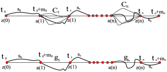
Figure 6: Scheme of $\mathcal{A},\mathcal{B}_{C}$ on top and of $\mathcal{A},\mathcal{B}_{g}$ on bottom.

Since we assume $\mathbf{P}_{\mathbf{z}(0)}[\mathcal{A},\mathcal{B}_{C}]>0$, we have that each $C_{i}$ consists of paths with the constraints above. Using (A) with $W_{i}=C_{i}$ and $W_{i}=\{g_{i}\}$ we get

$$\mathbf{P}_{\mathbf{z}(0)}[\mathcal{A},\mathcal{B}_{g}|\mathcal{A},\mathcal{B}_{C}]=\prod_{i=1}^{n}\bigl{(}\mathbf{P}_{\mathbf{a}(i)}\bigl{[}S(0,\tau_{\mathbf{z}(i)})=g_{i}\bigr{]}/\mathbf{P}_{\mathbf{a}(i)}\bigl{[}S(0,\tau_{\mathbf{z}(i)})\in C_{i}\bigr{]}\bigr{)},$$

and are done.

Proposition A.2

Let $\mathcal{X},\mathcal{Y}$ be events in some probability space, and let $\{\mathcal{Y}_{\alpha}\}_{\alpha\in I}$ be a partition of $\mathcal{Y}$ where $\forall\alpha\in I,\Pr[\mathcal{Y}_{\alpha}]>0$. Then for some $\gamma,\Gamma\in I$,

$$\Pr[\mathcal{X}|\mathcal{Y}_{\gamma}]\leq\Pr[\mathcal{X}|\mathcal{Y}]\leq\Pr[\mathcal{X}|\mathcal{Y}_{\Gamma}].$$

Follows from the identity,

$$\Pr[\mathcal{X}|\mathcal{Y}]=\sum_{\alpha\in I}\Pr[\mathcal{X}|\mathcal{Y}_{\alpha}]\Pr[\mathcal{Y}_{\alpha}]/\Pr[\mathcal{Y}].$$

Recall $\mathcal{J}_{B}[b]$ from Definition 5.5.

Lemma A.3

Let $B=B(n)$, let $b\in\sigma(B)$, where we write $m=\|b\|$. There is a $c_{\Lambda}(d)>0$, independent of $n$, such that for any $\mathbf{a}\in A(B),\mathbf{z}\in Z(B)$ and all large $n$,

$$\mathbf{P}_{\mathbf{a}}\bigl{[}\mathcal{J}_{B}[b]|\tau_{\partial B^{7}}=\tau_{\mathbf{z}}\bigr{]}>c_{\Lambda}\biggl{(}\frac{m}{n}\biggr{)}^{d-2}.$$

For $\mathbf{y}=(y_{1},\ldots,y_{d})\in\mathbb{Z}^{d}$, define $\mathcal{B}(\mathbf{y})$ to be the event $S(\cdot)$ hits $b$ at $\mathbf{y}$ and then the first coordinate of $S(\cdot)$ hits $y_{1}+4m$ and then hits $y_{1}-8m$, while the maximal change in the other coordinates is less than $m$. Let $\tau_{\mathcal{B}}(\mathbf{y})=\inf\{t\geq 0\dvtx S(0,t)\subset\mathcal{B}(\mathbf{y})\}$ be the first time the occurrence of $\mathcal{B}(\mathbf{y})$ is implied by $S(t)$. By Proposition A.5 for some $\mathbf{x}\in b$,

$$\mathbf{P}_{\mathbf{a}}\bigl{[}\tau_{b},\tau_{\mathcal{B}}\bigl{(}S(\tau_{b})\bigr{)}<\tau_{\partial B^{7}}|\tau_{\partial B^{7}}=\tau_{\mathbf{z}}\bigr{]}$$

$$\qquad\geq\mathbf{P}_{\mathbf{a}}[\tau_{b}<\tau_{\partial B^{7}}|\tau_{\partial B^{7}}=\tau_{\mathbf{z}}]\mathbf{P}_{\mathbf{x}}\bigl{[}\tau_{\mathcal{B}}(\mathbf{x})<\tau_{\partial B^{7}}|\tau_{\partial B^{7}}=\tau_{\mathbf{z}}\bigr{]}.$$

Using Lemma A.4 together with Corollary A.11, we have

$$\mathbf{P}_{\mathbf{a}}[\tau_{b}<\tau_{\partial B^{7}}|\tau_{\partial B^{7}}=\tau_{\mathbf{z}}]>c_{1}\biggl{(}\frac{m}{n}\biggr{)}^{d-2}.$$

Since $\{\tau_{\mathcal{B}}(\mathbf{x})<\tau_{\partial B^{7}}\}\subset\mathcal{J}_{B}[b]$, we are done if we show for some $c_{2}(d)>0$

$$\mathbf{P}_{\mathbf{x}}\bigl{[}\tau_{\mathcal{B}}(\mathbf{x})<\tau_{\partial B^{7}}|\tau_{\partial B^{7}}=\tau_{\mathbf{z}}\bigr{]}>c_{2}.$$ (33)

Partitioning over $S(\tau_{\mathcal{B}}(\mathbf{x}))\in b^{10}$ and using the Markov property, we have for some $\mathbf{y}\in b^{10}$,

$$\mathbf{P}_{\mathbf{x}}\bigl{[}\tau_{\mathcal{B}}(\mathbf{x})<\tau_{\partial B^{7}}|\tau_{\partial B^{7}}=\tau_{\mathbf{z}}\bigr{]}\mathbf{P}_{\mathbf{x}}[\tau_{\partial B^{7}}=\tau_{\mathbf{z}}]$$

(34)

$$\qquad\geq\mathbf{P}_{\mathbf{x}}\bigl{[}\tau_{\mathcal{B}}(\mathbf{x})<\tau_{\partial B^{7}}\bigr{]}\mathbf{P}_{\mathbf{y}}[\tau_{\partial B^{7}}=\tau_{\mathbf{z}}].$$

By the invariance principle, $\mathbf{P}_{\mathbf{x}}[\tau_{\mathcal{B}}(\mathbf{x})<\tau_{\partial B^{7}}]$ is bounded away from zero by a dimensional constant independent of $\mathbf{x}$. Since $\mathbf{x},\mathbf{y}$ from (A) are contained in $B^{6}$ for all large $n$, we use Lemma A.10 to get (33). In the lemma below, we look at the number vertices hit in an interior set $M\subset B^{6}$ by a $B$-traversal, and lower bound the probability for this number to be small in terms of $|M|$.

Lemma A.4

Let $B=B(n)$, let $M\subset B^{6}$, set $\mathbf{a}\in B^{7}$ and $\mathbf{z}\in Z(B)$. Let $X(M)=|\{\mathbf{v}\in M\dvtx\tau_{\mathbf{v}}<\tau_{\partial B^{7}}\}|$ and let $\mu_{X}=\mu_{X}(\mathbf{a},\mathbf{z})=\mathbf{E}_{\mathbf{a}}[X(M)|\tau_{\partial B^{7}}=\tau_{\mathbf{z}}]$. There is a $c_{1}(d)>0$, independent of $n$, $\mathbf{a}$ and $\mathbf{z}$, such that for all large $n$

$$\mathbf{P}_{\mathbf{a}}\bigl{[}X(M)\geq\tfrac{1}{2}\mu_{X}|\tau_{\partial B^{7}}=\tau_{\mathbf{z}}\bigr{]}>c_{1}\mu_{X}|M|^{-2/d}.$$

Thus, if $\mathbf{P}_{\mathbf{a}}[\tau_{\mathbf{v}}<\tau_{\partial B^{7}}|\tau_{\partial B^{7}}=\tau_{\mathbf{z}}]>f(n)$ for every $\mathbf{v}\in M$, then since $X(M)=\sum_{\mathbf{v}\in M}\mathbf{1}_{\{\tau_{\mathbf{v}}<\tau_{\partial B^{7}}\}}$, we have

$$\mathbf{P}_{\mathbf{a}}\bigl{[}X(M)\geq\tfrac{1}{2}\mu_{X}|\tau_{\partial B^{7}}=\tau_{\mathbf{z}}\bigr{]}>c_{1}|M|^{1-2/d}f(n).$$

Write $\mu_{X^{2}}$ for $\mathbb{E}_{\mathbf{a}}[X^{2}|\tau_{\partial B^{7}}=\tau_{\mathbf{z}}]$. By the Paley–Zygmund inequality, $\mathbf{P}_{\mathbf{a}}[X\geq\frac{1}{2}\mu_{X}]\geq\frac{1}{4}\mu_{X}^{2}/\mu_{X^{2}}$, so enough to show

$$\mu_{X^{2}}<Cm^{2}\mu_{X},$$

where $m=|M|^{1/d}$.

By linearity,

$$\mu_{X^{2}}=\sum_{\mathbf{v}\in M}\sum_{\mathbf{w}\in M}\mathbf{P}_{\mathbf{a}}[\tau_{\mathbf{w}},\tau_{\mathbf{v}}<\tau_{\partial B^{7}}|\tau_{\partial B^{7}}=\tau_{\mathbf{z}}].$$

For two vertices $\mathbf{x},\mathbf{y,}$ let $\tau_{\mathbf{v},\mathbf{w}}=\inf\{t\geq\tau_{\mathbf{x}}\dvtx S(t)=\mathbf{y}\}$. By a union bound

$$\mathbf{P}_{\mathbf{a}}[\tau_{\mathbf{w}},\tau_{\mathbf{v}}<\tau_{\partial B^{7}}|\tau_{\partial B^{7}}=\tau_{\mathbf{z}}] \leq \mathbf{P}_{\mathbf{a}}[\tau_{\mathbf{w}}\leq\tau_{\mathbf{w},\mathbf{v}}<\tau_{\partial B^{7}}|\tau_{\partial B^{7}}=\tau_{\mathbf{z}}]$$

$${}+\mathbf{P}_{\mathbf{a}}[\tau_{\mathbf{v}}\leq\tau_{\mathbf{v},\mathbf{w}}<\tau_{\partial B^{7}}|\tau_{\partial B^{7}}=\tau_{\mathbf{z}}].$$

By Bayes theorem and the Markov property,

$$\mathbf{P}_{\mathbf{a}}[\tau_{\mathbf{w}}\leq\tau_{\mathbf{w},\mathbf{v}}<\tau_{\partial B^{7}}|\tau_{\partial B^{7}}=\tau_{\mathbf{z}}]$$

$$\qquad=\frac{\mathbf{P}_{\mathbf{a}}[\tau_{\mathbf{w}}<\tau_{\partial B^{7}}|\tau_{\partial B^{7}}=\tau_{\mathbf{z}}]\mathbf{P}_{\mathbf{a}}[\tau_{\mathbf{w}}\leq\tau_{\mathbf{w},\mathbf{v}}<\tau_{\partial B^{7}}=\tau_{\mathbf{z}}|\tau_{\mathbf{w}}<\tau_{\partial B^{7}}]}{\mathbf{P}_{\mathbf{a}}[\tau_{\partial B^{7}}=\tau_{\mathbf{z}}|\tau_{\mathbf{w}}<\tau_{\partial B^{7}}]}$$

$$\qquad=\mathbf{P}_{\mathbf{a}}[\tau_{\mathbf{w}}<\tau_{\partial B^{7}}|\tau_{\partial B^{7}}=\tau_{\mathbf{z}}]\mathbf{P}_{\mathbf{w}}[\tau_{\mathbf{v}}<\tau_{\partial B^{7}}|\tau_{\partial B^{7}}=\tau_{\mathbf{z}}].$$

Again by the Markov property,

$$\mathbf{P}_{\mathbf{w}}[\tau_{\mathbf{v}}<\tau_{\partial B^{7}}|\tau_{\partial B^{7}}=\tau_{\mathbf{z}}]=\frac{\mathbf{P}_{\mathbf{v}}[\tau_{\partial B^{7}}=\tau_{\mathbf{z}}]\mathbf{P}_{\mathbf{w}}[\tau_{\mathbf{v}}<\tau_{\partial B^{7}}]}{\mathbf{P}_{\mathbf{w}}[\tau_{\partial B^{7}}=\tau_{\mathbf{z}}]}.$$

So by Lemma A.10, since $\mathbf{v},\mathbf{w}\in M\subset B^{6}$,

$$\mathbf{P}_{\mathbf{w}}[\tau_{\mathbf{v}}<\tau_{\partial B^{7}}|\tau_{\partial B^{7}}=\tau_{\mathbf{z}}]<C\mathbf{P}_{\mathbf{w}}[\tau_{\mathbf{v}}<\tau_{\partial B^{7}}]<C\mathbf{P}_{\mathbf{w}}[\tau_{\mathbf{v}}<\infty].$$

Thus, by symmetry,

$$\mu_{X^{2}}\leq 2\sum_{\mathbf{w}\in M}\mathbf{P}_{\mathbf{a}}[\tau_{\mathbf{w}}<\tau_{\partial B^{7}}|\tau_{\partial B^{7}}=\tau_{\mathbf{z}}]\sum_{\mathbf{v}\in M}C\mathbf{P}_{\mathbf{w}}[\tau_{\mathbf{v}}<\infty].$$

By Markov’s inequality, $\mathbf{P}_{\mathbf{w}}[\tau_{\mathbf{v}}<\infty]<G(\mathbf{w},\mathbf{v})$ where $G(\cdot,\cdot)$ is the Green’s function of a simple random walk on $\mathbb{Z}^{d}$. Standard estimates for $G(\cdot,\cdot)$ (see, e.g., Theorem 1.5.4 in lawler1996intersections ) give that $\mathbf{P}_{\mathbf{w}}[\tau_{\mathbf{v}}<\infty]<C(d)\|\mathbf{w}-\mathbf{v}\|_{2}^{2-d}$, and thus

$$\sum_{\mathbf{v}\in M}\mathbf{P}_{\mathbf{w}}[\tau_{\mathbf{v}}<\infty]<\sum_{\mathbf{v}\in M}\|\mathbf{w}-\mathbf{v}\|_{2}^{2-d}.$$

For some $\hat{c}(d)<\infty$, and all $r>0$, a ball of radius $\hat{c}r$ around the origin contains at least $r^{d}$ vertices in $\mathbb{Z}^{d}$. Since the RHS above can only be increased by moving a vertex in $M$ closer to $\mathbf{w}$, we have

$$\sum_{\mathbf{v}\in M}\mathbf{P}_{\mathbf{w}}[\tau_{\mathbf{v}}<\infty]<\hat{C}\sum_{r=1}^{\hat{c}m}r^{d-1}r^{2-d}<Cm^{2}=C|M|^{2/d}.$$

Since $\mu_{X}=\sum_{\mathbf{w}\in M}\mathbf{P}_{\mathbf{a}}[\tau_{\mathbf{w}}<\tau_{\partial B^{7}}|\tau_{\partial B^{7}}=\tau_{\mathbf{z}}]$, we are done. Let $\tau_{0}\dvtx(\mathbb{Z}^{d})^{\mathbb{Z}^{\geq 0}}\to\mathbb{Z}^{\geq 0}$ be a stopping time for the random walk $S(t)$. We denote by $\tau_{0}^{t}$ the stopping time on the $t$-time shifted sequences, that is, $\tau_{0}^{t}(\mathbf{a}_{0},\mathbf{a}_{1},\ldots)=\tau_{0}(\mathbf{a}_{t},\mathbf{a}_{t+1},\ldots)+t$. We call $\tau_{0}$ a simple stopping time if $\tau_{0}^{t}\geq\tau_{0}$ for every $t\geq 0$.

Proposition A.5

Let $B=B(n)$, set $\mathbf{a}\in B^{7}$ and $\mathbf{z}\in Z(B)$. Let $\tau_{1},\tau_{2}$ be simple stopping times (see above). Then there exists a $\mathbf{x}$ satisfying $\mathbf{P}_{\mathbf{a}}[S(\tau_{1})=\mathbf{x},\tau_{1}<\tau_{\partial B^{7}}|\tau_{\partial B^{7}}=\tau_{\mathbf{z}}]>0$ such that

$$\mathbf{P}_{\mathbf{a}}[\tau_{1},\tau_{2}\leq\tau_{\partial B^{7}}|\tau_{\partial B^{7}}=\tau_{\mathbf{z}}]\geq\mathbf{P}_{\mathbf{a}}[\tau_{1}<\tau_{\partial B^{7}}|\tau_{\partial B^{7}}=\tau_{\mathbf{z}}]\mathbf{P}_{\mathbf{x}}[\tau_{2}\leq\tau_{\partial B^{7}}|\tau_{\partial B^{7}}=\tau_{\mathbf{z}}].$$

Let

$$\pi_{\mathbf{y}}=\mathbf{P}_{\mathbf{a}}\bigl{[}S(\tau_{1})=\mathbf{y},\tau_{1}<\tau_{\partial B^{7}}|\tau_{\partial B^{7}}=\tau_{\mathbf{z}}\bigr{]}.$$

For $\mathbf{y}$ satisfying $\pi_{\mathbf{y}}>0$, we have by Bayes

$$\mathbf{P}_{\mathbf{a}}\bigl{[}\tau_{1},\tau_{2}\leq\tau_{\partial B^{7}},S(\tau_{1})=\mathbf{y}|\tau_{\partial B^{7}}=\tau_{\mathbf{z}}\bigr{]}$$

(35)

$$\qquad=\frac{\pi_{\mathbf{y}}\mathbf{P}_{\mathbf{a}}[\tau_{1},\tau_{2}\leq\tau_{\partial B^{7}}=\tau_{\mathbf{z}}|S(\tau_{1})=\mathbf{y},\tau_{1}<\tau_{\partial B^{7}}]}{\mathbf{P}_{\mathbf{a}}[\tau_{\partial B^{7}}=\tau_{\mathbf{z}}|S(\tau_{1})=\mathbf{y},\tau_{1}<\tau_{\partial B^{7}}]}.$$

Since $\tau_{2}$ is a simple stopping time,

$$\mathbf{P}_{\mathbf{a}}\bigl{[}\tau_{1},\tau_{2}\leq\tau_{\partial B^{7}}=\tau_{\mathbf{z}}|S(\tau_{1})=\mathbf{y},\tau_{1}<\tau_{\partial B^{7}}\bigr{]}$$

$$\qquad\geq\mathbf{P}_{\mathbf{a}}\bigl{[}\tau_{1}\leq\tau_{2}^{\tau_{1}}\leq\tau_{\partial B^{7}}=\tau_{\mathbf{z}}|S(\tau_{1})=\mathbf{y},\tau_{1}<\tau_{\partial B^{7}}\bigr{]}.$$

Plugging the above into (A) and using the strong Markov property, we get

$$\mathbf{P}_{\mathbf{a}}\bigl{[}\tau_{1},\tau_{2}\leq\tau_{\partial B^{7}},S(\tau_{1})=\mathbf{y}|\tau_{\partial B^{7}}=\tau_{\mathbf{z}}\bigr{]}\geq\pi_{\mathbf{y}}\mathbf{P}_{\mathbf{y}}[\tau_{2}\leq\tau_{\partial B^{7}}|\tau_{\partial B^{7}}=\tau_{\mathbf{z}}].$$

Let $\mathbf{x}\in\{\mathbf{y}\dvtx\pi_{\mathbf{y}}>0\}$ be the vertex for which $\mathbf{P}_{\mathbf{x}}[\tau_{2}\leq\tau_{\partial B^{7}}|\tau_{\partial B^{7}}=\tau_{\mathbf{z}}]$ is minimal. Summing both sides over $\{\mathbf{y}\dvtx\pi_{\mathbf{y}}>0\}$, we are done. We quote the Harnack principle for $\mathbb{Z}^{d}$ from Theorem 1.7.6 in lawler1996intersections .

Proposition A.6

Let $U$ be a compact subset of $\mathbb{R}^{d}$ contained in a connected open set $V$. Then there exists a $c=c(U,V)<\infty$ such that if $A_{n}=nU\cap\mathbb{Z}^{d}$, $D_{n}=nV\cap\mathbb{Z}^{d}$, and $f\dvtx D_{n}\cup\partial D_{n}\to[0,\infty)$ is harmonic in $D_{n}$, then

$$f(x)\leq cf(y),x,y\in A_{n}.$$

Lemma A.7

Let $B=B(n)$ and let $F$ be the union of all hyperplanes in $\mathbb{Z}^{d}$ that intersect $B^{6}$ and are parallel to $Z(B)$. There is a $C>0$ such that for any $\mathbf{y}\in Z(B)\cup A^{+}(B)$ and any $\mathbf{v}\in F\cap B^{7}$,

$$\mathbf{P}_{\mathbf{v}}[\tau_{\partial B^{7}}=\tau_{\mathbf{y}}]<Cn^{1-d}.$$

We prove for $\mathbf{y}\in Z(B)$. The proof $A^{+}(B)$ is the same so we omit it. Let $H$ be the infinite hyperplane in $\mathbb{Z}^{d}$ that contains $Z(B)$, and let $H_{0}$ a parallel hyperplane, which is the component of $\partial_{B^{7}}F$ closer to $Z(B)$. Let $h(\mathbf{y})$ be the $l_{1}$-closest vertex to $\mathbf{y}$ in $H_{0}$. By vertex transitivity, there is a function $g(n)$ such that for any $\mathbf{y}\in Z(B)$, $\mathbf{P}_{h(\mathbf{y})}[\tau_{H}=\tau_{\mathbf{y}}]=g(n)$. Observe that $\mathbf{P}_{(\cdot)}[\tau_{H}=\tau_{\mathbf{y}}]$ is a nonnegative harmonic function in the component of $\mathbb{Z}^{d}\setminus H$ containing $H_{0}$, so by the Harnack principle for $\mathbb{Z}^{d}$ (Proposition A.6), for some $c>0$, any $\mathbf{v}\in F\cap B^{7},\mathbf{y}\in Z(B)$ satisfies

$$c\mathbf{P}_{\mathbf{v}}[\tau_{H}=\tau_{\mathbf{y}}]>\mathbf{P}_{h(\mathbf{y})}[\tau_{H}=\tau_{\mathbf{y}}]=g(n).$$

Summing both sides over $\mathbf{y}\in Z(B)$, we get

$$g(n)<Cn^{1-d}.$$

Since $\{\tau_{\partial B^{7}}=\tau_{\mathbf{y}}\}\subset\{\tau_{H}=\tau_{\mathbf{y}}\}$, another application of the Harnack principle finishes the proof.

Corollary A.8

Let $B=B(n)$. There is a $C>0$ such that for any $\mathbf{a}\in A(B),\mathbf{z}\in Z(B)$

$$\mathbf{P}_{\mathbf{a}}[\tau_{\mathbf{z}}=\tau_{\partial B^{7}}]<Cn^{-d}.$$

Using the notation of Lemma A.7, by the Markov property $F$

$$\mathbf{P}_{\mathbf{a}}[\tau_{\mathbf{z}}=\tau_{\partial B^{7}}]=\sum_{\mathbf{x}}\mathbf{P}_{\mathbf{a}}\bigl{[}\tau_{F}<\tau_{\partial B^{7}},S(\tau_{F})=\mathbf{x}\bigr{]}\mathbf{P}_{\mathbf{x}}[\tau_{\mathbf{z}}=\tau_{\partial B^{7}}].$$

The right term is uniformly bounded by $Cn^{1-d}$ by Lemma A.7. Summing over $\mathbf{x}$, the event $\{\tau_{F}<\tau_{\partial B^{7}}\}$ implies that a one dimensional random walk starting at $1$ hits $n$ before hitting $0$, an event of probability $n^{-1}$.

Proposition A.9

Let $B=B(n)$. There is a $c(d)>0$ such that for any $A\subset\mathbb{Z}^{d}$ and $\mathbf{v,}\mathbf{w}\in\mathbb{Z}^{d}\setminus A$

$$c<\frac{\mathbf{P}_{\mathbf{v}}[\tau_{\mathbf{w}}<\tau_{A}]}{\mathbf{P}_{\mathbf{w}}[\tau_{\mathbf{v}}<\tau_{A}]}<c^{-1}.$$

Write $G_{A}(\mathbf{v},\mathbf{w})$ for the Green’s function of a random walk killed on hitting $A$, that is, the expected number of visits to $\mathbf{w}$ for a walk starting at $\mathbf{v}$ before it hits $A$. By elementary Markov theory, we have symmetry of Green’s function, $G_{A}(\mathbf{v},\mathbf{w})=G_{A}(\mathbf{w},\mathbf{v})$ and the following identity:

$$\mathbf{P}_{\mathbf{v}}[\tau_{\mathbf{w}}<\tau_{\partial B^{7}}]G_{A}(\mathbf{w},\mathbf{w})=\mathbf{P}_{\mathbf{w}}[\tau_{\mathbf{v}}<\tau_{\partial B^{7}}]G_{A}(\mathbf{v},\mathbf{v}).$$

For any $\mathbf{v}\in\mathbb{Z}^{d}\setminus A$, $G_{A}(\mathbf{v},\mathbf{v})\geq 1$, and is bounded above by the reciprocal of the probability a simple random walk never returns to $\mathbf{v}$, which by transience in $d>2$, is a finite dimensional constant.

Lemma A.10

Let $B=B(n)$. There is a $c>0$ such that for any $\mathbf{a}\in A(B),\mathbf{z}\in Z(B)$ and any $\mathbf{x}\in B^{6}$,

$$cn^{1-d}<\mathbf{P}_{\mathbf{a}}[\tau_{\mathbf{x}}<\tau_{\partial B^{7}}],\qquad\mathbf{P}_{\mathbf{x}}[\tau_{\mathbf{z}}=\tau_{\partial B^{7}}]<c^{-1}n^{1-d}.$$ (36)

Let $D_{\mathbf{x}}(r)=\{\mathbf{v}\in\mathbb{Z}^{d}\dvtx\|\mathbf{v}-\mathbf{x}\|_{2}\leq r\}$. Lemma 1.7.4 in lawler1996intersections tells us there is a $c_{1}(d)>0$ such that for any $\mathbf{r}\in\partial D_{\mathbf{0}}(r)$,

$$\mathbf{P}_{\mathbf{0}}[\tau_{\partial D_{\mathbf{0}}(r)}=\tau_{\mathbf{r}}]>c_{1}n^{1-d}.$$ (37)

Fix $\mathbf{y}\in A^{+}(B)$. Then there is a $\mathbf{v}\in B^{6}$ such that $\mathbf{y}\in\partial D_{\mathbf{v}}(n),D_{\mathbf{v}}(n)\subset B^{7}$. Since $\{\tau_{\partial D_{\mathbf{v}}(n)}=\tau_{\mathbf{y}}\}$ implies $\{\tau_{\partial B^{7}}=\tau_{\mathbf{y}}\}$, we get that

$$\mathbf{P}_{\mathbf{v}}[\tau_{\partial B^{7}}=\tau_{\mathbf{y}}]>c_{1}n^{1-d}.$$ (38)

The probability to exit $B^{7}$ at $\mathbf{y}$ is a nonnegative harmonic function in $B^{7}$. Thus, by the Harnack principle for $\mathbb{Z}^{d}$ (Proposition A.6), and since $c_{1}$ is independent of $\mathbf{y}$, the above is true for any $\mathbf{v}\in B^{6}$ and any $\mathbf{y}\in A^{+}(B)$ with an appropriate constant $c_{2}>0$ replacing $c_{1}$.

The same argument proves the lower bound in (36) for $\mathbf{P}_{\mathbf{x}}[\tau_{\mathbf{z}}=\tau_{\partial B^{7}}]$.

Next, by Proposition A.9 we have $\mathbf{P}_{\mathbf{a}}[\tau_{\mathbf{x}}<\tau_{\partial B^{7}}]>c\mathbf{P}_{\mathbf{x}}[\tau_{\mathbf{a}}<\tau_{\partial B^{7}}]$. Let $\mathbf{a}^{+}$ be $\mathbf{a}$’s neighbor in $A^{+}(B)$. Since $\{\tau_{\mathbf{a}}<\tau_{\partial B^{7}}\}\supset\{\tau_{\mathbf{a}^{+}}=\tau_{\partial B^{7}}\}$ and by (38), we get

$$\mathbf{P}_{\mathbf{x}}[\tau_{\mathbf{a}}<\tau_{\partial B^{7}}]\geq\mathbf{P}_{\mathbf{x}}[\tau_{\mathbf{a}^{+}}=\tau_{\partial B^{7}}]>cn^{1-d},$$

which proves the lower bound in (36) for $\mathbf{P}_{\mathbf{a}}[\tau_{\mathbf{x}}<\tau_{\partial B^{7}}]$ as well.

The upper bound for $\mathbf{P}_{\mathbf{x}}[\tau_{\mathbf{z}}=\tau_{\partial B^{7}}]$ is immediate from Lemma A.7. To prove for $\mathbf{P}_{\mathbf{a}}[\tau_{\mathbf{x}}<\tau_{\partial B^{7}}]$, we first use the lemma to get

$$\mathbf{P}_{\mathbf{x}}[\tau_{\mathbf{a}^{+}}=\tau_{\partial B^{7}}]<Cn^{1-d},$$

which implies the bound for $\mathbf{P}_{\mathbf{x}}[\tau_{\mathbf{a}}<\tau_{\partial B^{7}}]$, since by the Markov property, the probability for exiting $B^{7}$ one step after hitting $\mathbf{a}$ for the first time is

$$\mathbf{P}_{\mathbf{x}}[\tau_{\mathbf{a}}<\tau_{\partial B^{7}}]\cdot\frac{1}{2d}\leq\mathbf{P}_{\mathbf{x}}[\tau_{\mathbf{a}^{+}}=\tau_{\partial B^{7}}].$$

Using Proposition A.9 again, we get the bound with a new factor for $\mathbf{P}_{\mathbf{a}}[\tau_{\mathbf{x}}<\tau_{\partial B^{7}}]$.

Corollary A.11

Let $B=B(n)$. There is a $c>0$ such that for any $\mathbf{a}\in A(B)\cup B^{6},\mathbf{z}\in Z(B)$ and any $\mathbf{x}\in B^{6}$,

$$\mathbf{P}_{\mathbf{a}}[\tau_{\mathbf{x}}<\tau_{\partial B^{7}}|\tau_{\partial B^{7}}=\tau_{\mathbf{z}}]>cn^{2-d}.$$ (39)

By the Markov property,

$$\mathbf{P}_{\mathbf{a}}[\tau_{\mathbf{x}}<\tau_{\partial B^{7}}|\tau_{\partial B^{7}}=\tau_{\mathbf{z}}]\mathbf{P}_{\mathbf{a}}[\tau_{\partial B^{7}}=\tau_{\mathbf{z}}] = \mathbf{P}_{\mathbf{a}}[\tau_{\partial B^{7}}=\tau_{\mathbf{z}}|\tau_{\mathbf{x}}<\tau_{\partial B^{7}}]\mathbf{P}_{\mathbf{a}}[\tau_{\mathbf{x}}<\tau_{\partial B^{7}}]$$

$$= \mathbf{P}_{\mathbf{x}}[\tau_{\partial B^{7}}=\tau_{\mathbf{z}}]\mathbf{P}_{\mathbf{a}}[\tau_{\mathbf{x}}<\tau_{\partial B^{7}}].$$

If $\mathbf{a}\in A(B)$, then Lemma A.10 and Corollary A.8 give the bound. If $\mathbf{a}\in B^{6}$, then Lemma A.10 gives us the LHS is greater than $c\mathbf{P}_{\mathbf{a}}[\tau_{\mathbf{x}}<\tau_{\partial B^{7}}]$.

For $r>0$, let $\mathfrak{b}^{r}=\{\mathbf{x}\in\mathbb{R}^{d}\dvtx\forall i,1\leq i\leq d,|x_{i}|<r/2\}$ and for $\mathbf{y}\in\mathbb{R}^{d}$ let $\mathfrak{d}(\mathbf{y},r)=\{\mathbf{x}\in\mathbb{R}^{d}\dvtx\|\mathbf{x}-\mathbf{y}\|_{2}<r\}$. Choose $K(d)$ points $\mathbf{y}_{1},\ldots,\mathbf{y}_{K}\in\mathfrak{b}^{6}$ such that $\mathfrak{b}^{6}\subset\bigcup_{i=1}^{K}\mathfrak{d}(\mathbf{y}_{i},0.1)\subset\mathfrak{b}^{6.1}$. Let $D_{i}^{\alpha}(n)=\mathfrak{d}(n\mathbf{y}_{i},\alpha n)\cap\mathbb{Z}^{d}$. Then for $\alpha\geq 0.1$ and all $n$

$$B^{6}\subset\bigcup_{i=1}^{K}D_{i}^{\alpha}\subset B^{6+\alpha}.$$

Let $p_{\mathbf{a}}(\mathbf{x})=\mathbf{P}_{\mathbf{a}}[\tau_{\mathbf{x}}<\tau_{\partial B^{7}}]$. To show $p_{\mathbf{a}}(\mathbf{x})>cn^{2-d}$ uniformly in $\mathbf{x},\mathbf{a}\in B^{6}$, it is enough to show, w.l.o.g., that there is a $c_{1}>0$ such that for any $\mathbf{x}\in D_{1}^{0.1},\mathbf{a}\in B^{6}$, $p_{\mathbf{a}}(\mathbf{x})>c_{1}n^{2-d}$. Since $p_{\mathbf{a}}(\mathbf{x})$ is harmonic as a function of $\mathbf{a}$ in $B^{7}\setminus\{\mathbf{x}\}$, by the maximum (minimum) principle,

$$\min_{\mathbf{a}\in D_{1}^{0.2}\setminus\{\mathbf{x}\}}p_{\mathbf{a}}(\mathbf{x})\geq\min_{\mathbf{a}\in\partial D_{1}^{0.2}\cup\{\mathbf{x}\}}p_{\mathbf{a}}(\mathbf{x}).$$

Since $p_{\mathbf{x}}(\mathbf{x})=1$, and $\partial D_{1}^{0.2}\subset B^{6.5}$, it is thus enough to lower bound $p_{\mathbf{a}}(\mathbf{x})$ for $\mathbf{a}\in B^{6.5}\setminus D_{1}^{0.2}$. Since $p_{\mathbf{a}}(\mathbf{x})$ is harmonic and positive in $B^{7}\setminus D_{1}^{0.1}$, by the Harnack principle for $\mathbb{Z}^{d}$ (Proposition A.6), there is a $c_{2}(d)>0$ such that for any $\mathbf{a},\mathbf{b}\in B^{6.5}\setminus D_{1}^{0.2}$

$$p_{\mathbf{b}}(\mathbf{x})\geq c_{2}p_{\mathbf{a}}(\mathbf{x}).$$

Thus, it is enough to bound for some fixed $\mathbf{a}\in\partial D_{1}^{0.2}\cap B^{6}$. Let $D_{*}=\mathfrak{d}(\mathbf{a},0.6n)\cap\mathbb{Z}^{d}$ and note that $\mathbf{x}\in D_{*}\subset B^{7}$, implying $p_{\mathbf{a}}(\mathbf{x})\geq\mathbf{P}_{\mathbf{a}}[\tau_{\mathbf{x}}<\tau_{\partial D_{*}}]$. By Proposition 1.5.9 in lawler1996intersections , since $\mathbf{x}\in\mathfrak{d}(\mathbf{a},0.4n)\cap\mathbb{Z}^{d}$, $\mathbf{P}_{\mathbf{x}}[\tau_{\mathbf{a}}<\tau_{\partial D_{*}}]\geq cn^{2-d}$, and by Proposition A.9 we are done.

Appendix B Distance bound

In this section, we prove the following theorem.

Theorem B.1

Let $\omega_{0}\subset\mathcal{T}(N)$. If $\omega_{0}\subset\mathcal{T}(N)$ is $(N,k,\rho)$-good (see Section 2.5) where $k\geq 1,\rho>0$, then there is a $C(k,\rho)<\infty$ such that for all large $N$ and any two vertices $\mathbf{x},\mathbf{y}\in\omega_{0}$

$$d_{\omega_{0}}(\mathbf{x},\mathbf{y})<Cd_{\mathcal{T}}(\mathbf{x},\mathbf{y})\log^{(k-1)}N+C(\log N)^{4d+2},$$

where $\log^{(m)}N$ is $\log(\cdot)$ iterated $m$ times of $N$.

We start by reducing from the torus to top-level.boxes. To prove the theorem, it is enough to show that there exists a $C(k,\rho)<\infty$ such that for all large $n$, any $\omega\in\mathcal{G}_{k}^{\rho}(n)$ and any $\mathbf{x},\mathbf{y}\in\omega\cap b^{5}(n)$ satisfy

$$d_{\omega}(\mathbf{x},\mathbf{y})<Cd_{b^{7}(n)}(\mathbf{x},\mathbf{y})\log^{(k-1)}n+C(\log n)^{4d+2}.$$ (40)

Note that while $\omega_{0}$ is a subgraph of $\mathcal{T}$ as far as graph distance, we require (40) to hold for $\omega$ as a subgraph of $\mathbb{Z}^{d}$ (no wrap around). To see why this is enough, let $\mathbf{x},\mathbf{y}\in\mathcal{T}(N)$ and set $n=\lceil N/10\rceil$. First assume there is a top-level box $b_{*}(\mathbf{a},n)$ and $\hat{\mathbf{x}},\hat{\mathbf{y}}\in b_{*}^{3}$ such that $\mathbf{x}=\Pi_{N}(\hat{\mathbf{x}}),\mathbf{y}=\Pi_{N}(\hat{\mathbf{y}})$. Let $\omega=\Pi_{N}^{-1}(\omega_{0})\cap b_{*}^{7}$. Note $d_{\omega}(\hat{\mathbf{x}},\hat{\mathbf{y}})\geq d_{\omega_{0}}(\mathbf{x},\mathbf{y})$ but since $\|b_{*}^{3}\|<N/2$,$d_{b_{*}^{7}}(\hat{\mathbf{x}},\hat{\mathbf{y}})=d_{\mathcal{T}}(\mathbf{x},\mathbf{y})$. By (40), since $b_{*}$ is $(\Pi_{N}^{-1}(\omega_{0}),k,\rho)$-good by definition, we are done. If no such $b_{*}$ exists, then by our construction of top-level boxes, $d_{\mathcal{T}}(\mathbf{x},\mathbf{y})>n$. Let $b_{\mathbf{x}},b_{\mathbf{y}}$ be the top-level boxes such that $\mathbf{x}\in b_{\mathbf{x}},\mathbf{y}\in b_{\mathbf{y}}$. We can make a $\Delta$-connected path of top-level boxes from $\mathbf{x}$ to $\mathbf{y}$ of length at most $10d$. Since $b_{1},b_{2}$ that are $\Delta$-neighbors satisfy that $b_{1}\subset b_{2}^{5}$, by Remark 2.6, (40) implies the theorem.

To simplify notation, we fix $k,\rho,n$ and $\omega\in\mathcal{G}_{k}^{\rho}(n)$ for the remainder of the section. We write $\mathcal{G}_{i}$ (resp., $i$-good) for $\mathcal{G}_{i}^{\rho\Lambda^{k-i}}$ [resp., $(\omega,i,\rho\Lambda^{k-i})$-good].

We now utilize the recursive goodness properties of $\omega$ to extract a single connected cluster of $\omega$ which is a power of log $\omega$-distance from its complement in $\omega$ and is “nicely” embedded in $\mathbb{Z}^{d}$. Given an $(i+1)$-good box $B$ where $0\leq i<k$, we write

$$\mathcal{S}(B,i)=\bigl{\{}b\in\sigma(B)\dvtx b\mbox{ is }i\mbox{-good}\bigr{\}},$$

and let $\sigma_{B}=\|\Delta(\sigma(B))\|=|\sigma(B)|^{{1}/{d}}$. Since $B$ is $(i+1)$-good, by definition we have that $\Delta\mathcal{S}(B,i)\in\mathcal{P}(\sigma_{B})$. Thus, there exists a good cluster $\mathcal{C}(\Delta\mathcal{(S}(B,i)))$ satisfying Percolation properties 1, 2, 3 (see Section 2.3). Let $\mathbf{C}_{i}(B)\subset\sigma(B)$ be the set for which $(\Delta\mathbf{C}_{i}(B))=\mathcal{C}(\Delta(\mathcal{S}(B,i)))$. For $i=0,\ldots,k$ let us define $\beta_{i}=\beta_{i}(\omega,n)$. Set $\beta_{k}=\{B(n)\}$ and for $i=k-1,\ldots,0$ recursively define $\beta_{i}=\{b\in\mathbf{C}_{i}(B)\dvtx B\in\beta_{i+1}\}$. See Figure 7 for a schematic illustration.

Let $n_{j}=s^{(k-j)}(n)$. Thus, for $b\in\beta_{j}$ we have $\|b\|=n_{j}$ and also $|\sigma(b)|^{{1}/{d}}<6n_{j}/n_{j-1}$ for all large $n$. Note that by Percolation property 1, $\{\beta_{j}(n)\}_{j=0}^{k}$ are nonempty for all large $n$. Roughly, $\bigcup\beta_{0}$ is the nicely embedded cluster referred to above. Its precise properties follow.

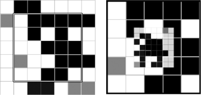
Figure 7: On the left is a schematic example of $B^{7}(n)$ where the black boxes represent $\beta_{k}=\mathbf{C}_{k-1}(B(n))$ and the gray ones $\mathcal{S}(B,k-1)\setminus\beta_{k}$. On the right is a blowup of the framed region on the left where the small black boxes are a part of $\beta_{k-1}$.

Given an $(i+1)$-good box $B$, let $\mathbf{C}_{i}^{5}(B)=\{b\in\mathbf{C}_{i}(B)\dvtx b\cap B^{5}\neq\varnothing\}$.

Lemma B.2

Set $b_{k}=B(n)$. There is a $C(k)$ such that for any $\mathbf{x}_{k}\in b_{k}^{5}\cap\omega$, there are boxes $\{b_{i}\}_{i=0}^{k-1}$ satisfying: (i) $b_{i}\in\mathbf{C}_{i}^{5}(b_{i+1})\subset\beta_{i}$, and (ii) there is a $\mathbf{x}_{0}\in\omega\cap b_{0}$ such that

$$d_{\omega}(\mathbf{x}_{k},\mathbf{x}_{0})<C(k)(\log n)^{4d+2}.$$

We use backward induction. For $1\leq j\leq k$, we prove that if $\mathbf{x}_{j}\in B_{j}^{5}\cap\omega$ where $B_{j}\in\beta_{j}$, then there is a $b_{j-1}\in\mathbf{C}_{j-1}^{5}(B_{j})\subset\beta_{j-1}$ and a $\mathbf{x}_{j-1}\in b_{j-1}$ satisfying

$$d_{\omega}(\mathbf{x}_{j},\mathbf{x}_{j-1})<c(d)n_{j-1}^{d}(\log n_{j})^{2}.$$ (41)

Since the conditions of the lemma provide us with an initial $\mathbf{x}_{k}\in B^{5}(n)$ where by definition $B(n)\in\beta_{k}$, the bound on $d_{\omega}(\mathbf{x}_{k},\mathbf{x}_{0})$ is proved by connecting $\mathbf{x}_{k},\mathbf{x}_{k-1},\ldots,\mathbf{x}_{0}$.

We assumed $B_{j}\in\beta_{j}$, so in particular, $B_{j}$ is $j$-good. Let $b_{*}\in\sigma(B_{j})$ be the subbox of $B_{j}$ containing $\mathbf{x}_{j}$ and assume $b_{*}\notin\mathbf{C}_{j-1}^{5}(B_{j})$ as otherwise we are done. Consider

$$\mathbf{B}=\bigl{\{}b\in B_{\Delta}\bigl{(}b_{*},\log\bigl{|}\sigma(B_{j})\bigr{|}\bigr{)}\dvtx b\cap B_{j}^{5}\neq\varnothing\bigr{\}}.$$

Since $b_{*}\cap B_{j}^{5}\neq\varnothing$ by assumption, $|\mathbf{B}|>\log^{2}|\sigma(B_{j})|$, and thus by Percolation property 2 (see Section 2.3), there is a $b_{j-1}\in\mathbf{B}\cap\mathbf{C}_{j-1}^{5}(B_{j})$. Thus, there is a $\Delta$-path $\mathbf{p}\subset\sigma(B_{j})$ of length at most $d\log|\sigma(B_{j})|$ starting at $b_{*}$ and ending at $b_{j-1}$. By Remark 2.6 on $\mathcal{G}_{0}^{\rho}$ (see Section 2.4), for any $\Delta$-neighboring boxes $b_{\alpha},b_{\beta}$ in the path, $\omega\cap b_{\alpha}$ is connected to $\omega\cap b_{\beta}$ in $\omega\cap b_{\alpha}^{+}$. Choosing some $\mathbf{x}_{j-1}\in\omega\cap b_{j-1}$ and using the volume of $\bigcup_{b\in\mathbf{p}}b^{7}$ as a trivial distance bound, we get (41). For $0\leq j<k$, note that although $\|b_{1}\|=\|b_{2}\|$ for any $b_{1},b_{2}\in\beta_{j}$, since they can be subboxes of different $B_{1},B_{2}$, $b_{1}$ is not in general an element of $\operatorname{sp}\{b_{2}\}$. Thus, for each $0\leq j\leq k$, we add a graph structure to $\beta_{j}$ by defining a neighbor relation ($\stackrel{{\scriptstyle 5}}{{\sim}}$) between boxes $b_{1},b_{2}\in\beta_{j}$. We define that $b_{1}\stackrel{{\scriptstyle 5}}{{\sim}}b_{2}$ if and only if $b_{1}\subset b_{2}^{5}$ and $b_{2}\subset b_{1}^{5}$. Note this relation is reflexive, and that for $(j+1)$-good $B$ and $b_{1},b_{2}\in\mathbf{C}_{j}(B)$, $d_{\beta_{j}}(b_{1},b_{2})\leq d_{\Delta}(b_{1},b_{2})$. For the remainder of the section, any graph properties of $\beta_{j}$ referred to, such as connectivity or distance, use the graph structure created by $\stackrel{{\scriptstyle 5}}{{\sim}}$.

Lemma B.3

There is a $C_{d}$ such that for each $0<j\leq k$, if $B_{1},B_{2}\in\beta_{j}$ are $\stackrel{{\scriptstyle 5}}{{\sim}}$-connected, and we have $b_{1}\in\mathbf{C}_{j-1}^{5}(B_{1}),b_{2}\in\mathbf{C}_{j-1}^{5}(B_{2})$, then$d_{\beta_{j-1}}(b_{1},b_{2})<C_{d}(d_{\beta_{j}}(B_{1},B_{2})\vee 1)n_{j}/n_{j-1}$. In particular, $b_{1},b_{2}$ are $\stackrel{{\scriptstyle 5}}{{\sim}}$-connected in $\beta_{j-1}$.

We prove the lemma for the special case of $B_{1}\stackrel{{\scriptstyle 5}}{{\sim}}B_{2}$ [i.e., $d_{\beta_{j}}(B_{1},\break B_{2})\leq 1$]. The general lemma follows by applying the neighbor case over a path in $\beta_{j}$ realizing the $\stackrel{{\scriptstyle 5}}{{\sim}}$-distance between two fixed boxes. By definition, $\mathbf{C}_{j-1}(B_{1})$ and $\mathbf{C}_{j-1}(B_{2})$ are each $\Delta$-connected sets, and thus $\stackrel{{\scriptstyle 5}}{{\sim}}$-connected. By Percolation property 3, for $i=1,2$ and any $b,b^{\prime}\in\mathbf{C}_{j-1}^{5}(B_{i})$, $d_{\mathbf{C}_{j-1}(B_{i})}(b,b^{\prime})<C_{d}n_{j}/n_{j-1}$. Since $\mathbf{C}_{j-1}(B_{i})\subset\beta_{j-1}$ and $\stackrel{{\scriptstyle 5}}{{\sim}}$-distance is at most $\Delta$-distance, to complete the proof it is enough to show existence of $\hat{b}_{1}\in\mathbf{C}_{j-1}^{5}(B_{1})$ and $\hat{b}_{2}\in\mathbf{C}_{j-1}^{5}(B_{2})$ such that $\hat{b}_{1}\subset\hat{b}_{2}^{5}$ and $\hat{b}_{2}\subset\hat{b}_{1}^{5}$. For $i=1,2$, let $\mathbf{D}_{i}=\{b\in\sigma(B_{i})\dvtx b\subset B_{2}\}$ and let $\mathbf{E}_{i}=\mathbf{D}_{i}\cap\mathbf{C}_{j-1}(B_{i})$. Let $D_{i}=\bigcup\mathbf{D}_{i}$ and let $E_{i}=\bigcup\mathbf{E}_{i}$. Since $E_{i}\subset D_{i}$, we have $B_{2}\setminus E_{i}=(B_{2}\setminus D_{i})\cup(D_{i}\setminus E_{i})$. By a volume bound, $|B_{2}\setminus D_{i}|\leq 2dn_{j-1}n_{j}^{d-1}$ and by Percolation property 1, $|\mathbf{D}_{i}\setminus\mathbf{E}_{i}|<10^{-d}|\sigma(B_{i})|$. Since $|\sigma(B_{i})|^{{1}/{d}}<6n_{j}/n_{j-1}$, this implies $|D_{i}\setminus E_{i}|<(0.6n_{j})^{d}$. As $|B_{2}|=n_{j}^{d}$ and $d>2$, we have by the bound on $|B_{2}\setminus E_{i}|$ for $i=1,2$ that there is a $\mathbf{x}\in E_{1}\cap E_{2}$. The containing boxes $\mathbf{x}\in\hat{b}_{i}\in\mathbf{C}_{j-1}(B_{i})$ for $i=1,2$ are thus $\stackrel{{\scriptstyle 5}}{{\sim}}$-neighbors. We now prove the theorem by showing there exists a $C(k,\rho)<\infty$ such that for any $\mathbf{x},\mathbf{y}\in\omega\cap B^{5}(n)$, (40) holds for all large $n$. Proof of Theorem B.1 We demonstrate there is a path from $\mathbf{x}$ to $\mathbf{y}$ in $\omega$ shorter than the RHS of (40). Let $b_{\mathbf{x},k}=B(n)$ and apply Lemma B.2 to $\mathbf{x}$ to get boxes $\{b_{\mathbf{x},i}\}_{i=0}^{k-1}$ satisfying: (i) $b_{\mathbf{x},i}\in\mathbf{C}_{i}^{5}(b_{\mathbf{x},i+1})\subset\beta_{i}$, and (ii) there is a $\mathbf{x}_{0}\in\omega\cap b_{\mathbf{x},0}$ such that $d_{\omega}(\mathbf{x},\mathbf{x}_{0})<C(k)(\log n)^{4d+2}$. Observe that (i) implies $\mathbf{x}_{0}\in b_{\mathbf{x},k-1}^{6}$ for all large $n$. Set $b_{\mathbf{y},k}=B(n)$ and apply the lemma to $\mathbf{y}$ as well to get $b_{\mathbf{y},i}$ and $\mathbf{y}_{0}$ with analogous properties.

By Lemma B.3, $\beta_{k-1}$ is $\stackrel{{\scriptstyle 5}}{{\sim}}$-connected, and more specifically,

$$d_{\beta_{k-2}}(b_{\mathbf{x},k-2},b_{\mathbf{y},k-2})<C_{d}\bigl{(}d_{\beta_{k-1}}(b_{\mathbf{x},k-1},b_{\mathbf{y},k-1})\vee 1\bigr{)}\frac{n_{k-1}}{n_{k-2}}.$$

Iterating the lemma, we get

$$d_{\beta_{0}}(b_{\mathbf{x},0},b_{\mathbf{y},0})<C_{d}^{k-1}\bigl{(}d_{\beta_{k-1}}(b_{\mathbf{x},k-1},b_{\mathbf{y},k-1})\vee 1\bigr{)}\frac{n_{k-1}}{n_{0}}.$$ (42)

Since $b_{\mathbf{x},k-1},b_{\mathbf{y},k-1}\in\mathbf{C}_{k-1}^{5}(B(n))$, by Percolation property 3

$$\quad d_{\mathbf{C}_{k-1}(B(n))}(b_{\mathbf{x},k-1},b_{\mathbf{y},k-1})<c_{a}d_{\sigma(B(n))}(b_{\mathbf{x},k-1},b_{\mathbf{y},k-1})\vee c_{a}\log\frac{n_{k}}{n_{k-1}}.$$ (43)

Where both are defined, $\stackrel{{\scriptstyle 5}}{{\sim}}$-distance is at most $\Delta$-distance, and thus we may replace $d_{\mathbf{C}_{k-1}(B(n))}(\cdot,\cdot)$ in (43) by $d_{\beta_{k-1}}(\cdot,\cdot)$. Since $n_{k-1}\cdot d_{\sigma(B(n))}(\cdot,\cdot)$ and $d_{B^{7}(n)}(\cdot,\cdot)$ are comparable, and using that $\mathbf{x}_{0}\in b_{\mathbf{x},k-1}^{6},\mathbf{y}_{0}\in b_{\mathbf{y},k-1}^{6}$ we have

$$n_{k-1}d_{\beta_{k-1}}(b_{\mathbf{x},k-1},b_{\mathbf{y},k-1})<c_{a}^{\prime}\bigl{(}d_{B^{7}(n)}(\mathbf{x}_{0},\mathbf{y}_{0})\vee n_{k-1}\log n_{k}\bigr{)}.$$

Plugging this into (42), we get

$$d_{\beta_{0}}(b_{\mathbf{x},0},b_{\mathbf{y},0})<C(k)\bigl{(}d_{B^{7}(n)}(\mathbf{x}_{0},\mathbf{y}_{0})\vee\log^{5}n\bigr{)}/n_{0}.$$

By properties of $\mathcal{G}_{0}^{\rho}$ (see Section 2.4), vertices in $\stackrel{{\scriptstyle 5}}{{\sim}}$-neighboring boxes in $\beta_{0}$ are connected in $\omega$ in a path which is at most twice the volume of one box, and thus we get

$$d_{\omega}(\mathbf{x}_{0},\mathbf{y}_{0})<C(k)\bigl{(}d_{B^{7}(n)}(\mathbf{x}_{0},\mathbf{y}_{0})\vee\log^{5}n\bigr{)}(n_{0})^{d-1}.$$

We pay a $C(\log n)^{4d+2}$ term to connect $\mathbf{x},\mathbf{y}$ to $\mathbf{x}_{0},\mathbf{y}_{0}$, respectively. This terms also absorbs the $(n_{0})^{d-1}\log^{5}n$ factor above. Since $(n_{0})^{d-1}$ is$o(\log^{(k-1)}n)$, we are done.

Appendix C Random interlacements notation

We try to follow as much as possible the canonical notation of Alain-Sol Sznitman MR2680403 . Let $W$ and $W_{+}$ be the spaces of doubly infinite and infinite trajectories in $\mathbb{Z}^{d}$ that spend only a finite amount of time in finite subsets of $\mathbb{Z}^{d}$:

$$W = \Bigl{\{}\gamma\dvtx\mathbb{Z}\to\mathbb{Z}^{d};\bigl{|}\gamma(n)-\gamma(n+1)\bigr{|}=1,\forall n\in\mathbb{Z};\lim_{n\to\pm\infty}\bigl{|}\gamma(n)\bigr{|}=\infty\Bigr{\}},$$

$$W_{+} = \Bigl{\{}\gamma\dvtx{\mathbb{N}}\to\mathbb{Z}^{d};\bigl{|}\gamma(n)-\gamma(n+1)\bigr{|}=1,\forall n\in\mathbb{Z};\lim_{n\to\infty}\bigl{|}\gamma(n)\bigr{|}=\infty\Bigr{\}}.$$

The canonical coordinates on ${W}$ and ${W}_{+}$ will be denoted by $X_{n}$, $n\in{\mathbb{Z}}$ and $X_{n}$, $n\in{\mathbb{N}}$, respectively. Here, we use the convention that ${\mathbb{N}}$ includes $0$. We endow $W$ and $W_{+}$ with the sigma-algebras ${\mathcal{W}}$ and ${\mathcal{W}}_{+}$, respectively, which are generated by the canonical coordinates. For $\gamma\in W$, let range $(\gamma)=\gamma({\mathbb{Z}})$. Furthermore, consider the space $W^{*}$ of trajectories in $W$ modulo time shift:

$$W^{*}=W/\sim\qquad\mbox{where }w\sim w^{\prime}\Longleftrightarrow w(\cdot)=w^{\prime}(\cdot+k)\mbox{ for some }k\in\mathbb{Z}.$$

Let $\pi^{*}$ be the canonical projection from $W$ to $W^{*}$, and let ${\mathcal{W}}^{*}$ be the sigma-algebra on $W^{*}$ given by $\{A\subset W^{*}\dvtx(\pi^{*})^{-1}(A)\in{\mathcal{W}}\}$. Given $K\subset{\mathbb{Z}}^{d}$ and $\gamma\in W_{+}$, let $\tilde{H}_{K}(\gamma)$ denote the hitting time of $K$ by $\gamma$:

$$\tilde{H}_{K}(\gamma)=\inf\bigl{\{}n\geq 1\dvtx X_{n}(\gamma)\in K\bigr{\}}.$$ (44)

For $x\in{\mathbb{Z}}^{d}$, let $P_{x}$ be the law on $(W_{+},{\mathcal{W}}_{+})$ corresponding to simple random walk started at $x$, and for $K\subset{\mathbb{Z}}^{d}$, let $P_{x}^{K}$ be the law of simple random walk, conditioned on not hitting $K$. Define the equilibrium measure of $K$:

$$e_{K}(x)=\cases{P_{x}[\tilde{H}_{K}=\infty],&\quad$x\in K,$\vspace*{2pt}\cr 0,&\quad$x\notin K.$}$$ (45)

Define the capacity of a set $K\subset{\mathbb{Z}}^{d}$ as

$$\operatorname{cap}(K)=\sum_{x\in{\mathbb{Z}}^{d}}e_{K}(x).$$ (46)

Next, we define a Poisson point process on $W^{*}\times{\mathbb{R}}_{+}$. The intensity measure of the Poisson point process is given by the product of a certain measure $\nu$ and the Lebesque measure on ${\mathbb{R}}_{+}$. The measure $\nu$ was constructed by Sznitman in MR2680403 , and now we characterize it. For $K\subset{\mathbb{Z}}^{d}$, let $W_{K}$ denote the set of trajectories in $W$ that enter $K$. Let $W_{K}^{*}=\pi^{*}(W_{K})$ be the set of trajectories in $W^{*}$ that intersect $K$. Define $Q_{K}$ to be the finite measure on $W_{K}$ such that for $A,B\in{\mathcal{W}}_{+}$ and $x\in{\mathbb{Z}}^{d}$,

$$Q_{K}\bigl{[}(X_{-n})_{n\geq 0}\in A,X_{0}=x,(X_{n})_{n\geq 0}\in B\bigr{]}=P_{x}^{K}[A]e_{K}(x)P_{x}[B].$$ (47)

The measure $\nu$ is the unique $\sigma$-finite measure such that

$${\mathbh{1}}_{W^{*}_{K}}\nu=\pi^{*}\circ Q_{K}\qquad\forall K\subset{\mathbb{Z}}^{d}\mbox{ finite}.$$ (48)

The existence and uniqueness of the measure was proved in Theorem 1.1 of MR2680403 . Consider the set of point measures in $W^{*}\times{\mathbb{R}}_{+}$:

$$\Omega = \Biggl{\{}\omega=\sum_{i=1}^{\infty}\delta_{(w_{i}^{*},u_{i})};w_{i}^{*}\in W^{*},u_{i}\in{\mathbb{R}}_{+},$$

$$\hskip 8.0pt\omega\bigl{(}W_{K}^{*}\times[0,u]\bigr{)}<\infty,\mbox{ for every finite }K\subset\mathbb{Z}^{d}\mbox{ and }u\in{\mathbb{R}}_{+}\Biggr{\}}.$$

Also consider the space of point measures on $W^{*}$:

$$\quad\tilde{\Omega}=\Biggl{\{}\sigma=\sum_{i=1}^{\infty}\delta_{w_{i}^{*}};w_{i}^{*}\in W^{*},\sigma\bigl{(}W_{K}^{*}\bigr{)}<\infty,\mbox{ for every finite }K\subset\mathbb{Z}^{d}\Biggr{\}}.$$ (50)

For $u>u^{\prime}\geq 0$, we define the mapping $\omega_{u^{\prime},u}$ from $\Omega$ into $\tilde{\Omega}$ by

$$\omega_{u^{\prime},u}=\sum_{i=1}^{\infty}\delta_{w_{i}^{*}}{{\mathbh{1}}}\bigl{\{}u^{\prime}\leq u_{i}\leq u\bigr{\}}\qquad\mbox{for }\omega=\sum_{i=1}^{\infty}\delta_{(w_{i}^{*},u_{i})}\in\Omega.$$ (51)

If $u^{\prime}=0$, we write $\omega_{u}$. On $\Omega$ we let ${\mathbb{P}}$ be the law of a Poisson point process with intensity measure given by $\nu(dw^{*})\,dx$. Observe that under ${\mathbb{P}}$, the point process $\omega_{u,u^{\prime}}$ is a Poisson point process on $\tilde{\Omega}$ with intensity measure $(u-u^{\prime})\nu(dw^{*})$. Given $\sigma\in\tilde{\Omega}$, we define

$${\mathcal{I}}(\sigma)=\bigcup_{w^{*}\in\operatorname{supp}(\sigma)}\operatorname{range}\bigl{(}w^{*}\bigr{)}.$$ (52)

For $0\leq u^{\prime}\leq u$, we define

$${\mathcal{I}}^{u^{\prime},u}={\mathcal{I}}(\omega_{u^{\prime},u}),$$ (53)

which we call the random interlacement set between levels $u^{\prime}$ and $u$. In case $u^{\prime}=0$, we write ${\mathcal{I}}^{u}$.

Finally, we can define the measure of the random walk described in Theorem 2.3. Let $\mathbb{P}^{u}_{0}[\cdot]=\mathbb{P}[\cdot|0\in{\mathcal{I}}^{u}]$. For every ${\mathcal{I}}^{u}$ distributed according to $\mathbb{P}_{0}^{u}$, let $\mathbf{P}_{0}^{u}$ be the law of a SRW on ${\mathcal{I}}^{u}$ starting from $0$.

Appendix D Index of symbols by order of appearance

Symbol	Page	Definition
${\mathcal{T}}(N,d)$	2	$d$-dimensional torus.
$\Pi_{N}$	2	For $x\in\mathbb{Z}^{d}$, ${\mathcal{O}}_{N}(x)=(x_{1}\operatorname{mod}N,\ldots,x_{d}\operatorname{mod}N)$.
${\mathcal{R}}(t)$	2	The range of SRW on the torus.
$\partial$	2.1	Outer vertex boundary.
$\partial^{\mathrm{in}}$	2.1	Inner vertex boundary.
$B(\mathbf{x},n)$	2.2	$\{\mathbf{y}\in\mathbb{Z}^{d}\dvtx\forall i,1\leq i\leq d,-n/2\leq{\mathbf{x}}(i)-\mathbf{y}(i)<n/2\}$.
$\operatorname{sp}\{B(\mathbf{x},n)\}$	2.2	$\{B(\mathbf{x}+\sum_{i}\mathbf{e}_{i}k_{i}n,n)\dvtx(k_{1},\ldots,k_{d})\in\mathbb{Z}^{d}\}$.
$\Delta$	2.2	The isomorphism, $\Delta$: $\operatorname{sp}\{B\}\rightarrow\mathbb{Z}^{d}$.
$B^{\alpha}$	2.4	For a box $B=B(x,n)$, $B^{\alpha}=B(x,\alpha n)$.
$s(n)$	2.4	$\lceil\log n\rceil^{4}$.
$s^{(i)}(n)$	2.4	$s(\cdot)$ iterated $i$ times.
$\sigma(B(\mathbf{x},n))$	2.5	$\operatorname{sp}\{b(\mathbf{x},s(n))\}\cap\{b({\mathbf{y}},s(n))\dvtx\mathbf{y}\in B(x,5n+3\lceil\log n\rceil^{6})\}$.
${\mathcal{P}}(n)$	2.3	Percolation configurations.
${\mathcal{G}}_{k}^{\rho}(n)$	2.4	$k$-good configurations.
$\hat{\phi}(r)$	3.4	$\inf\{\Phi_{S}\dvtx N^{1/3}<\pi(S)\leq r\wedge(1-1/4d)|{\omega}_{0}|\}$.
$\Phi_{S}$	3	$\frac{Q(S,S^{c})}{\pi(S)}$.
$\Phi(u)$	3.4	$\inf\{\Phi_{S}\dvtx 0<\pi(S)\leq u\wedge\frac{1}{2}\}$.
Top, Bot	5.1	Top and bottom projections of $B^{3}$ on $B^{7}$.
B-$\mathit{traversal}$	5.1	An ordered pair $\eta=(a,z)$, $a\in\operatorname{Top}$, $z\in\operatorname{Bot}$.
B-$\mathit{itinerary}$	5.1	An ordered sequence of B-$\mathit{traversals}$.
$\tau_{\rho}(b)$	5.1	$\tau_{\rho}(b)=\gamma^{+}_{\lceil\rho n^{d-2}\rceil}$.
${\mathcal{D}}^{\rho}_{\Lambda\rho}$	5.5, 6.2	Each $b\in\sigma(B)$ is traversed top to bottom at least $\Lambda\rho\|b\|^{d-2}$ times.
${\mathcal{F}}_{N}^{T}(b,k,\rho)$	6	The event $\{b\cap{\mathcal{O}}_{N}^{-1}\circ{\mathcal{R}}_{N}(t)\in{\mathcal{G}}_{k}^{\rho}(n)\dvtx\forall t\geq T\}$.

References

(1){barticle}[mr]
\bauthor\bsnmAntal, \bfnmPeter\binitsP. and \bauthor\bsnmPisztora, \bfnmAgoston\binitsA.
(\byear1996).
\btitleOn the chemical distance for supercritical Bernoulli percolation.
\bjournalAnn. Probab.
\bvolume24
\bpages1036–1048.
\biddoi=10.1214/aop/1039639377, issn=0091-1798, mr=1404543
\bptokimsref\endbibitem
(2){barticle}[mr]
\bauthor\bsnmBenjamini, \bfnmItai\binitsI. and \bauthor\bsnmMossel, \bfnmElchanan\binitsE.
(\byear2003).
\btitleOn the mixing time of a simple random walk on the super
critical percolation cluster.
\bjournalProbab. Theory Related Fields
\bvolume125
\bpages408–420.
\biddoi=10.1007/s00440-002-0246-y, issn=0178-8051, mr=1967022
\bptokimsref\endbibitem
(3){barticle}[mr]
\bauthor\bsnmBenjamini, \bfnmItai\binitsI. and \bauthor\bsnmSznitman, \bfnmAlain-Sol\binitsA.-S.
(\byear2008).
\btitleGiant component and vacant set for random walk on a discrete torus.
\bjournalJ. Eur. Math. Soc. (JEMS)
\bvolume10
\bpages133–172.
\biddoi=10.4171/JEMS/106, issn=1435-9855, mr=2349899
\bptokimsref\endbibitem
(4){barticle}[mr]
\bauthor\bsnmBramson, \bfnmMaury\binitsM. and \bauthor\bsnmLebowitz, \bfnmJoel L.\binitsJ. L.
(\byear1991).
\btitleAsymptotic behavior of densities for two-particle annihilating
random walks.
\bjournalJ. Stat. Phys.
\bvolume62
\bpages297–372.
\biddoi=10.1007/BF01020872, issn=0022-4715, mr=1105266
\bptokimsref\endbibitem
(5){bmisc}[author]
\bauthor\bsnmČerný, \bfnmJ.\binitsJ. and \bauthor\bsnmPopov, \bfnmS.\binitsS.
(\byear2011).
\bhowpublishedOn the internal distance in the interlacement set.
\bptokimsref\endbibitem
(6){barticle}[mr]
\bauthor\bsnmDeuschel, \bfnmJean-Dominique\binitsJ.-D. and \bauthor\bsnmPisztora, \bfnmAgoston\binitsA.
(\byear1996).
\btitleSurface order large deviations for high-density percolation.
\bjournalProbab. Theory Related Fields
\bvolume104
\bpages467–482.
\biddoi=10.1007/BF01198162, issn=0178-8051, mr=1384041
\bptokimsref\endbibitem
(8){bbook}[author]
\bauthor\bsnmLawler, \bfnmG. F.\binitsG. F.
(\byear1996).
\btitleIntersections of Random Walks.
\bpublisherBirkhäuser,
\blocationBasel.
\bptokimsref\endbibitem
(9){bbook}[mr]
\bauthor\bsnmLawler, \bfnmGregory F.\binitsG. F. and \bauthor\bsnmLimic, \bfnmVlada\binitsV.
(\byear2010).
\btitleRandom Walk: A Modern Introduction.
\bseriesCambridge Studies in Advanced Mathematics
\bvolume123.
\bpublisherCambridge Univ. Press,
\blocationCambridge.
\bidmr=2677157
\bptokimsref\endbibitem
(10){barticle}[mr]
\bauthor\bsnmLiggett, \bfnmT. M.\binitsT. M.,
\bauthor\bsnmSchonmann, \bfnmR. H.\binitsR. H. and \bauthor\bsnmStacey, \bfnmA. M.\binitsA. M.
(\byear1997).
\btitleDomination by product measures.
\bjournalAnn. Probab.
\bvolume25
\bpages71–95.
\biddoi=10.1214/aop/1024404279, issn=0091-1798, mr=1428500
\bptokimsref\endbibitem
(11){bincollection}[mr]
\bauthor\bsnmLovász, \bfnmLászló\binitsL. and \bauthor\bsnmKannan, \bfnmRavi\binitsR.
(\byear1999).
\btitleFaster mixing via average conductance.
In \bbooktitleAnnual ACM Symposium on Theory of Computing
(Atlanta, GA, 1999)
\bpages282–287.
\bpublisherACM,
\blocationNew York.
\biddoi=10.1145/301250.301317, mr=1798047
\bptokimsref\endbibitem
(12){barticle}[mr]
\bauthor\bsnmMathieu, \bfnmPierre\binitsP. and \bauthor\bsnmRemy, \bfnmElisabeth\binitsE.
(\byear2004).
\btitleIsoperimetry and heat kernel decay on percolation clusters.
\bjournalAnn. Probab.
\bvolume32
\bpages100–128.
\biddoi=10.1214/aop/1078415830, issn=0091-1798, mr=2040777
\bptokimsref\endbibitem
(13){barticle}[mr]
\bauthor\bsnmMorris, \bfnmB.\binitsB. and \bauthor\bsnmPeres, \bfnmYuval\binitsY.
(\byear2005).
\btitleEvolving sets, mixing and heat kernel bounds.
\bjournalProbab. Theory Related Fields
\bvolume133
\bpages245–266.
\biddoi=10.1007/s00440-005-0434-7, issn=0178-8051, mr=2198701
\bptokimsref\endbibitem
(14){barticle}[mr]
\bauthor\bsnmPete, \bfnmGábor\binitsG.
(\byear2008).
\btitleA note on percolation on : Isoperimetric
profile via exponential cluster repulsion.
\bjournalElectron. Commun. Probab.
\bvolume13
\bpages377–392.
\biddoi=10.1214/ECP.v13-1390, issn=1083-589X, mr=2415145
\bptokimsref\endbibitem
(15){bmisc}[author]
\bauthor\bsnmProcaccia, \bfnmE. B.\binitsE. B. and \bauthor\bsnmRosenthal, \bfnmR.\binitsR.
(\byear2011).
\bhowpublishedConcentration estimates for the isoperimetric constant
of the super critical percolation cluster.
Preprint. Available at \arxivurlarXiv:1110.6006.
\bptokimsref\endbibitem
(16){barticle}[mr]
\bauthor\bsnmRáth, \bfnmBalázs\binitsB. and \bauthor\bsnmSapozhnikov, \bfnmArtëm\binitsA.
(\byear2011).
\btitleOn the transience of random interlacements.
\bjournalElectron. Commun. Probab.
\bvolume16
\bpages379–391.
\biddoi=10.1214/ECP.v16-1637, issn=1083-589X, mr=2819660
\bptokimsref\endbibitem
(17){barticle}[mr]
\bauthor\bsnmSznitman, \bfnmAlain-Sol\binitsA.-S.
(\byear2010).
\btitleVacant set of random interlacements and percolation.
\bjournalAnn. of Math. (2)
\bvolume171
\bpages2039–2087.
\biddoi=10.4007/annals.2010.171.2039, issn=0003-486X, mr=2680403
\bptokimsref\endbibitem