A Flexible Patch-Based Lattice Boltzmann
Parallelization Approach for Heterogeneous GPU–CPU Clusters

Abstract

Sustaining a large fraction of single GPU performance in parallel computations is considered to be the major problem of GPU-based clusters. In this article, this topic is addressed in the context of a lattice Boltzmann flow solver that is integrated in the WaLBerla software framework. We propose a multi-GPU implementation using a block-structured MPI parallelization, suitable for load balancing and heterogeneous computations on CPUs and GPUs. The overhead required for multi-GPU simulations is discussed in detail and it is demonstrated that the kernel performance can be sustained to a large extent. With our GPU implementation, we achieve nearly perfect weak scalability on InfiniBand clusters. However, in strong scaling scenarios multi-GPUs make less efficient use of the hardware than IBM BG/P and x86 clusters. Hence, a cost analysis must determine the best course of action for a particular simulation task. Additionally, weak scaling results of heterogeneous simulations conducted on CPUs and GPUs simultaneously are presented using clusters equipped with varying node configurations.

1 Introduction

In the field of computational fluid dynamics (CFD), flow solvers based on the lattice Boltzmann method (LBM) have become a well-established alternative for solving the Navier-Stokes equations directly. The LBM algorithm is a cellular automaton derived from the Boltzmann equation; each node (cell) on the computational grid exchanges information with its neighbors, which makes memory bandwidth the performance-limiting bottleneck of the LBM in most cases. Modeling real systems requires large computational effort, therefore performance optimization and parallelization of LBM codes are very active fields of research. GPU architectures offer the highest memory to processor chip bandwidth available today in commodity hardware and promise a big performance gain for memory-bound applications. However, tremendous effort has to be put into highly efficient LBM codes even on single GPUs [1, 2, 3]. First promising results of nonregular implementations [4] show that the LBM is applicable to nonuniform domains and multi-GPU clusters as well.

In order to push these experimental efforts into real production CFD applications it is crucial to establish scalable LBM codes on GPU clusters. Still the current Top500 list [5] contains only a few GPU clusters, since the nonstandard programming paradigm and the rather slow CPU-to-GPU connection are obstacles that hamper their general applicability. The main contribution of this paper is to show that it is possible to exploit the full computational power of currently emerging GPU–CPU clusters. We start by applying low-level optimizations to the GPU kernels to improve single-GPU performance, then move to multiple GPUs using MPI-based distributed memory parallelization, and finally establish load-balanced heterogeneous GPU–CPU parallelism by incorporating the otherwise idle multicore CPUs and GPU-less compute nodes into the flow solver.

To bring together high performance and high productivity we apply a Patch and Block design, which divides the computational domain into subregions that are distributed to the compute units (GPUs or teams of CPU threads in a multicore node). This is a choice as to how many subregions are assigned to each compute unit instead of individual cells, simplifying static load balancing. Ghost layers are exchanged between neighboring subregions using the appropriate data paths (shared memory, PCIe bus, InfiniBand interconnect). A simulation is thus able to run in parallel on a heterogeneous cluster comprising various different architectures. The whole code is included in the WaLBerla (Widely applicable lattice Boltzmann solver from Erlangen) software framework, which is employed in many CFD applications. We can show that high computational performance can be sustained within WaLBerla and therefore only very small application management and communication overhead is added.

This paper is organized as follows. We start with a brief description of the architectures used for measurements and the LBM method in Sec. 2. Code optimizations and performance models are shown in Sec. 3. Section 4 describes the WaLBerla software framework and the heterogeneous parallelization approach. In Sec. 5 we finally analyze the performance behavior of our code on single CPUs, single GPUs, and heterogeneous CPU–GPU clusters in strong and weak scaling scenarios.

2 Methods and Architectures

2.1 The Lattice Boltzmann Method

The LBM has evolved over the last two decades and is today widely accepted in academia and industry for solving incompressible flows. Coming from a simplified gas-kinetic description, i.e. a velocity discrete Boltzmann equation with an appropriate collision term, it satisfies the Navier-Stokes equations in the macroscopic limit with second order accuracy [6, 7]. In contrast to conventional computational fluid dynamic methods, the LBM uses a set of particle distribution functions (PDF) in each cell to describe the fluid flow. A PDF is defined as the expected value of particles in a volume located at the lattice position $\vec{x}$ with the lattice velocity $\vec{e}_{i}$. Computationally, the LBM is based on a uniform grid of cubic cells that are updated in each time step using an information exchange with nearest neighbor cells only. Structurally, this is equivalent to an explicit time stepping for a finite difference scheme. For the LBM the lattice velocities $\vec{e}_{i}$ determine the finite difference stencil, where $i$ represents an entry in the stencil. Here, we use the so-called D3Q19 model resulting in a $19$ point stencil and 19 PDFs in each cell. The evolution of a single PDF $f_{i}$ is described by

$$f_{i}(\vec{x}+\vec{e}_{i}\Delta t,t+\Delta t)=f^{\mathrm{coll}}_{i}(\vec{x},t)=$$

$$\ \ \ \ \ \ f_{i}(\vec{x},t)-\frac{1}{\tau}\big{[}f_{i}(\vec{x},t)-f_{i}^{\mathit{eq}}\left(\rho(\vec{x},t),\vec{u}(\vec{x},t)\right)\big{]}\qquad$$ (1)

$$f_{i}^{\mathit{eq}}\left(\rho(\vec{x},t),\vec{u}(\vec{x},t)\right)=w_{i}\left[\rho+\rho_{0}\left(3\vec{e}_{i}\vec{u}+4.5(\vec{e}_{i}\vec{u})^{2}-1.5\vec{u}^{2}\right)\right]$$ (2)

$$i=0\ldots 19,$$

and can be split into two steps: A collision step applying the collision operator and a propagation step advecting the PDFs to the neighboring cells. In this article, we use the single relaxation time collision operator [7]. In Eq. 1, $f_{i}^{\mathrm{coll}}$ denotes the intermediate state after collision but before propagation. The relaxation time $\tau$ can be determined from the kinematic viscosity $\nu=(\tau-\frac{1}{2})c_{s}^{2}\delta t$, with $c_{s}$ as the speed of sound. Further, $f^{eq}_{i}$ is a Taylor expanded version of the Maxwell-Boltzmann equilibrium distribution function [7] optimized for incompressible flows [8]. For the isothermal case, $f^{eq}_{i}$ depends on the macroscopic velocity $\vec{u}(\vec{x},t)$ and the macroscopic density $\rho(\vec{x},t)$, and the lattice weights $w_{i}$ are $\frac{1}{3}$, $\frac{1}{18}$ or $\frac{1}{36}$. The macroscopic quantities $\rho$ and $\vec{u}$ are determined from the $0^{th}$ and $1^{st}$ order moment of the distribution functions $\rho(\vec{x},t)=\rho_{0}+\delta\rho(\vec{x},t)=\sum_{i=0}^{18}f_{i}(\vec{x},t),$ and $\rho_{0}\vec{u}(\vec{x},t)=\sum_{i=0}^{18}{\vec{e}}_{i}f_{i}(\vec{x},t)$, where $\rho$ is split into a constant part $\rho_{0}$ and a slightly changing perturbation $\delta\rho$. The equation of state of an ideal gas provides the pressure $p(\vec{x},t)=c_{s}^{2}\rho(\vec{x},t)$.

Usually, the PDFs are initialized to $f_{i}^{\mathit{eq}}\left(\rho_{0},0\right)$. To increase the accuracy of simulations in single precision we use $\tilde{f}_{i}(\vec{x},t)=f_{i}(\vec{x},t)-f_{i}^{\mathit{eq}}\left(\rho_{0},0\right)$ and $\tilde{f}_{i}^{\mathit{eq}}\left(\rho(\vec{x},t),\vec{u}(\vec{x},t)\right)=f_{i}^{\mathit{eq}}\left(\rho(\vec{x},t),\vec{u}(\vec{x},t)\right)-f_{i}^{\mathit{eq}}\left(\rho_{0},0\right)$ as proposed by [8] resulting in PDF values centered around $0$. According to [1], it is possible with the LBM scheme described above to achieve accurate single precision results, which is important for GPU implementations.

A further important issue is the implementation of the propagation, for which there exist two schemes: First a pushing and second a pulling. For the first case, the PDFs in a cell are first collided and then pushed to the neighborhood. In the second case, the neighboring PDFs are first pulled into the lattice cell and then collided. Additionally, the propagation step introduces data dependencies to the LBM, which commonly result in an implementation of the LBM using two PDF grids. However, these dependencies are of local type, as only PDFs of neighboring cells are accessed. Hence, the LBM is particularly well suited for massively parallel simulations  [9, 10, 11]. In WaLBerla, we use the pull approach as it is better suited for our parallelization (see Sec. 4 for details on the parallelization).

The most common approach for implementing solid wall boundaries in the LBM is the bounce-back (BB) rule [6, 7], i.e. if a distribution is about to be propagated into a solid cell, the distribution’s direction is reversed into the original cell. BB generally assumes that the wall is in the middle between the two cell centers, i.e. half-way. This formulation leads to: $f_{\bar{i}}(\vec{x},t+\Delta t)=f_{i}(\vec{x},t)+6w_{i}\rho_{0}\vec{e}_{i}\vec{u}_{w}$ with $\vec{e}_{\bar{i}}=-\vec{e}_{i}$ and $u_{w}$ being the velocity prescribed at the wall.

2.2 Hardware Environments

2.2.1 CPU-based Cluster Systems

In general, current clusters based on dual-socket Intel quad-core processors offer a peak node performance in the range of $60$ to $100$ GFLOPS. The on-chip memory controllers with up to three DDR3 memory channels per socket provide a theoretical peak node bandwidth of $64$ GB/s. The clusters introduced in the following table all share this common architecture:
Nodes Processor Interconnect Clock Speed Memory nVIDIA GPUs per Node Xeon [GHz] [GB] TinyGPU [12] 8 X5550 DDR IB 2.66 24 2 x TESLA C1060 JUROPA [13] 2208 X5570 QDR IB 2.93 24 NEC Nehalem [14] 700 X5560 DDR IB ^∗ 2.8 12 2 x TESLA S1070 ^∗ Oversubscribed IB backbone (30 nodes)
The IBM BlueGene/P-based cluster JUGENE [15] comprises $73728$ compute nodes, each equipped with one $850$ MHz PowerPC $450$ quad-core processor and $4$ GB memory, which are connected via a proprietary high speed interconnect offering $850$ MB/s per link direction.

2.2.2 nVIDIA Graphic Processing Units

The GT–200-based GPUs are the second generation of nVIDIA graphics cards capable of GPGPU computing using the Compute Unified Device Architecture (CUDA) [16]. A GPU has several multiprocessors (MP), each with $8$ processor cores. Computations are executed by so-called threads, whereas up to $1024$ threads are concurrently running on one MP in order to hide memory latency by efficient scheduling. Threads are organized in GPU-blocks, which are pinned to an MP over the whole runtime. Each MP has $16384$ registers and $16$ kB of shared memory available, i.e. there are only $16$ registers and about $16$ bytes per thread if $1024$ threads are running in parallel. Hence, the concurrency is limited if kernels allocate more than $16$ registers, which has a severe impact on performance. See [17] for further details on CUDA and nVIDIA GPU hardware.

2.3 Interconnects

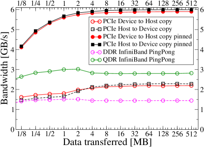
Figure 1: Host–GPU and MPI PingPong bandwidth measurements on TinyGPU. The function cudaMemcpy implementing a vector copy is used for all PCIe copy operations.

Most of today’s high performance systems use InfiniBand (IB) for the connection of the compute nodes. Heterogeneous computations on CPUs and GPUs require PCI-Express (PCIe) transfers for both IB and CPU–GPU communication. In order to develop a sensible performance model, all involved communication paths must be considered.

PCIe 2.0 x16 is currently the fastest peripheral bus with a peak transfer bandwidth of 8 GB/s per direction. Figure 1 shows that one can maintain about 6 GB/s bandwidth if the transfered data is larger than $2$ MB and the CUDA call cudahostalloc is used to allocate so-called pinned memory on the host. Pinned memory in contrast to memory allocated by malloc will not be paged out, is private to the process allocating it, and is local to the physical socket of the allocating process. The advantage of pinned memory results from the possibility to use fast direct-memory-accesses (DMA). With our current LBM implementation packets in the range of $250$ kB to $500$ kB are exchanged per PCIe data transfer, leading to an effective bandwidth between about $5$ GB/s and $6$ GB/s. Please note that two GPUs on the NEC Nehalem cluster have to share the same PCIe bus, which is capable of transferring $12.8$ GB/s.

IB host adapters are connected to the host via the PCIe x8 interface. IB bandwidth measurements of the Intel IMB PingPong benchmark [18] for quad-(QDR) and double-(DDR) data rate IB can be found in Fig. 1. The measurements show that QDR ($3.0$ GB/s) doubles the bandwidth compared to DDR ($1.5$ GB/s) and that the GPU’s PCIe operates with at least twice the bandwidth.

The performance of LBM codes is usually given in terms of million fluid lattice cell updates per second (MFLUPS) instead of GFlops, as the actual executed GFlops cannot be determined precisely. Table 1 gives an estimate for the minimal impact of the data transfer over all interconnects on performance. The compute time of the kernel $t_{k}$ and the IB and PCIe data transfer times $t_{t}$ can hereby be determined by

$$t_{k}=\frac{n_{cell}^{3}}{P}\ \ \ \ \mbox{and}\ \ \ \ t_{t}=\frac{2\cdot n_{cell}^{2}\cdot n_{PDF}\cdot n_{plane}\cdot s_{PDF}}{B},$$

where $P$ is the performance, $n_{Cell}$ the number of lattice cells per dimension, $n_{PDF}$ the number of PDFs communicated per boundary cell, $n_{plane}$ the number of planes to be communicated, $s_{PDF}$ the size in bytes of a PDF and $B$ is the bandwidth of the corresponding interconnect. It was assumed that all domain boundaries have to be communicated, which results in the transfer of $6$ boundary planes with $5$ PDFs per cell.

Steps	Tesla C1060 ($\sim 300$ MFLUPS)
Compute Time		3.3 ms
PCIe: 5 GB/s	(I)	0.48 ms
IB: 3.0 GB/s	(II)	0.8 ms
Total Time:	(I)	3.78 ms $\rightarrow$ 264 MFLUPS
	(I+II)	4.58 ms $\rightarrow$ 218 MFLUPS

Table 1: Performance estimates for multi-GPU single precision LBM simulations including InfiniBand and PCIe transfers of the complete boundary data. The estimated times are based on the obtainable bandwidth. A domain size of $100^{3}$ lattice cells is assumed for the example and the pure kernel performance has been taken from Fig. 2.

3 CPU and GPU Kernel Implementation

3.1 Upper Bound Performance Estimation

The performance of our LBM implementation is like most scientific codes dominated by memory bandwidth. To estimate an upper bound for the obtainable LBM bandwidth on CPUs, we employ the vector operation $c(:)=a(:)$ from the STREAM Benchmarks [19], which results in a memory bandwidth of $33$ GB/s on JUROPA. The CPU’s cache hierarchy and arithmetic units are fast enough so that computations and in-cache transfers are completely hidden by memory loads and stores. For the GPU bandwidth, we implemented our own benchmark, which achieved a maximum memory bandwidth of $78$ GB/s on a nVIDIA TESLA C1060, if the occupancy is at least $0.5$, i.e. if at least $512$ threads out of the maximum of $1024$ (GT–200) threads are scheduled per MP. Further benchmark details can be found in [2]. Furthermore, the bytes transferred for each LBM lattice cell update $n_{bytes}$ can be determined by [20]

$$n_{bytes}=n_{stencil}\cdot(n_{loads}+n_{store})\cdot s_{PDF},$$

where $n_{stencil}$ is the size of the LBM stencil, and $n_{loads}$ and $n_{stores}$ the number of load and stores. Due to the Read-for-Ownership, this results in $228$ bytes using single precision (SP) and $456$ bytes using double precision (DP) for the CPU, and $152$ (SP) / $304$ (DP) bytes for the GPU implementation. Thus, it is possible to estimate an upper limit for the LBM node performance. For one node on JUROPA we estimate a performance of $144$ (SP) / $72$ (DP) MFLUPS and $516$ (SP) / $258$ (DP) MFLUPS for one nVIDIA TESLA C1060.

3.2 Kernel Performance and Implementation Details

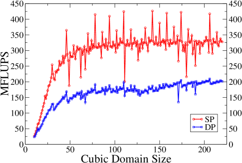
Figure 2: Single-GPU measurements of the pure GPU kernel performance for SP and DP on a nVIDIA TESLA C1060.

One key aspect for achieving a good LBM kernel performance is the data layout. There exist two major implementation strategies: The Array-of-Structure (AoS) and the Structure-of-Arrays (SoA) layout. For the AoS layout, the PDFs of each cell are stored adjacent in memory, whereas for the SoA Layout the PDFs pointing in the same lattice direction are adjacent in memory. Our CPU kernel implementation uses the AoS layout together with the pull streaming approach, and to improve the performance, arithmetic optimizations have been applied. In addition, the Patch and Block data structures introduced in Sec. 4.2 allow for the decomposition of the simulation domain into smaller subdomains, leading to an implicit spatial blocking. No further unrolling or spatial and temporal blocking is applied. Our implementation reaches up to $78$ (SP) / $55$ (DP) MFLUPS on one node of JUROPA and up to $7.3$ (SP) / $6.1$ (DP) on one node of JUGENE. This is slightly lower, but comparable to well-optimized solvers, e.g. [9]. The DP kernel is about 23 % off from the performance estimated before and still in agreement with the model. The large discrepancy of nearly 50 % for the SP kernel can be attributed to the computational intensity of the nonvectorized LBM kernel, making the code essentially not memory, but computationally bound.

In contrast to the CPU implementation, the GPU implementation uses the SoA layout, because in combination with the pull streaming approach it is possible to align the memory writes. In addition, the scattered loads that occur in our implementation can be efficiently coalesced by the memory subsystem. Hence, we do not have to use the shared memory of the GPU. For the scheduling of the threads, we adopted a scheme first proposed in [1], where each GPU thread updates one lattice cell and one GPU block is assigned one row of the simulation domain. In order to improve the kernel performance, we reduced the number of registers used for each thread by prefetching the PDFs into temporal variables and also by modifying the array accesses as described in [2]. With these optimizations, we can achieve a maximum occupancy of $0.5$. The maximum performance for some domain sizes has been around $500$ (SP) / $250$ (DP), which agrees well with our performance estimates and also with the results in [3]. A comparison to [1] is rather difficult as they used a different LBM stencil and hardware has evolved. Still, the sustained memory bandwidth of both implementations on the particular hardware is around $70$ % of peak bandwidth. A detailed kernel performance analysis for cubic domain sizes is depicted in Fig. 2. The measured performance fluctuations for varying domain sizes result from the different numbers of scheduled threads per MP and from memory alignment issues.

4 The WaLBerla Framework

WaLBerla is a massively parallel multiphysics software framework that is originally centered around the LBM, but whose applicability is not limited to this algorithm. Its main design goals are to provide excellent application performance across a wide range of computing platforms and the easy integration of new functionality. In this context additional functionality can either extend the framework for new simulation tasks, or optimize existing algorithms by adding special-purpose hardware-dependent kernels or new concepts such as load balancing strategies. In order to achieve this flexibility, WaLBerla has been designed utilizing software engineering concepts such as the spiral model and prototyping [21, 22], and also using common design patterns [23]. Several researchers and cooperation partners have already used the software framework to solve various complex simulation tasks. Amongst others, free-surface flows [24] using a localized parallel algorithm for bubbles coalescence, free-surface flows with floating objects [25], flows through porous media, clotting processes in blood vessels [26], particulate flows for several million volumetric particles [27] on up to $8192$ cores, and a fluctuating lattice Boltzmann [28] for nano fluids have been included. In addition to the strictly Eulerian view of field equations and their discretization, WaLBerla also supports Lagrangian representations of physical phenomena, such as e.g. particulate flows. Currently, the prototype WaLBerla $2.0$ is under development extending the framework for heterogeneous simulations on CPUs and GPUs, and load balancing strategies. Heterogeneous computations are already supported, but the designs for dynamic load balancing strategies are currently under development, although the underlying data structures can already be used for static load balancing.

In WaLBerla, all simulation tasks are broken down into several basic steps, so-called Sweeps. A Sweep can be divided into two parts: a communication step fulfilling the boundary conditions for parallel simulations by nearest neighbor communication and a communication independent work step traversing the process-local grid and performing operations on all cells. The work step usually consists of a kernel call, which is realized for instance by a function object or a function pointer. As for each work step there may exist a list of possible (hardware dependent) kernels, the executed kernel is selected by our functionality management (see below). For pure LBM simulations only one Sweep is needed exchanging PDF boundary data during the communication phase and executing one of the kernels that have been described in Sec. 3. The functionality management in WaLBerla $2.0$ selects the required kernels according to meta data provided with each kernel. This data allows the selection of different kernels for different simulation runs, processes and subregions of the simulation domain, so-called Blocks (see Sec. 4.2). Hence, it is possible to specifically select, for heterogeneous computations even on each single process, hardware optimized kernels. Further details on the functionality management can be found in Sec. 4.1.

A further fundamental design of the whole software framework is our Patch and Block data structure, which is a specific version of block-structured grids. Besides forming the basis for the parallelization and load balancing strategies, Blocks are also essential to configure the domain subregions with regard to the simulated task and the utilized hardware. More information on the Patch and Block data structure can be found in Sec. 4.2. Further, WaLBerla enables parallel MPI simulations of various simulation tasks. In order to do so, the process-to-process communication supports messages, containing data from any kind of data structure conforming to a documented interface, of arbitrary length and data type as well as the serialization of messages to the same process. Using our parallelization it is possible to represent even complex communication patterns, such as our localized bubble merge algorithm [24] or our parallel multigrid solver ported from [29]. The general parallelization design is described in Sec. 4.3. For parallel simulations on GPUs, the boundary data of the GPU has first to be copied by a PCIe transfer to the CPU and then be communicated via the MPI parallelization. Therefore, the data structures of the single core implementation are extended by buffers on GPU and CPU in order to achieve fast PCIe transfers. In addition, on-GPU copy kernels are added to fill these buffers. In Sec. 4.4 the details of our parallel GPU implementation are introduced. To support heterogeneous simulations on GPUs and CPUs, we execute different kernels on CPU and GPU and also define a common interface for the communication buffers, so that an abstraction from the hardware is possible. Additionally, the work load of the CPU and the GPU processes has to be balanced. In our approach this is achieved by allocating several Blocks on each GPU and only one on each CPU-only process.

4.1 Functionality Management

The functionality management in WaLBerla $2.0$ allows to select different functionality (e.g. kernels, communication functions) for different granularities, e.g. for the whole simulation, for individual processes, and for individual Blocks. This is realized by adding meta data to each functionality consisting of three unique identifiers (UID).

UID	Name	Granularity	Example
fs	Functionality Selector	Simulation	Gravity on/off
hs	Hardware Selector	Process	CPU and/or GPU
bs	Block Selector	Block	LBM

On the basis of these UIDs the kernels can be selected according to the requirements of the simulated scenarios. Hence, physical effects can be turned on/off in an efficient well-defined manner by means of the fs selector. Hardware-dependent kernels can be selected for different architectures depending on the hs selector and simulation tasks can be selected via the bs selector. A complex example for the capabilities of our concept are heterogeneous LBM simulations on CPUs and GPUs described in Sec. 4.5.

4.2 Patch and Block Concept

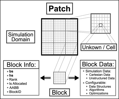
Figure 3: Patch and Block Design. Each Block stores management information consisting of a block and a hardware selector, a MPI rank, an axis aligned bounding box (AABB), and a Block identifier (BlockID) required for the identification of individual Blocks. The Blocks’ management information is stored on all processes, but simulation data is only allocated on processes which are responsible for that particular Block.

In WaLBerla the simulation domain is described with our Patch and Block design, which is illustrated in Fig. 3. It has been developed in order to support massively parallel simulations, load balancing strategies and the configuration to simulation tasks and hardware. A Patch hereby is a rectangular cuboid describing a region in the simulation that is discretized with the same resolution. In principal, these Patches can be arranged hierarchically for grid refinement techniques, but in this work we are using only one Patch covering the whole simulation domain. This Patch is further subdivided into a Cartesian grid of Blocks, again of cuboidal shape, containing the actual grid-based data for the simulation (simulation data). With the aid of these Blocks the simulation domain can be partitioned for parallel simulation. It is hereby possible to allocate several Blocks on a process in order to support load balancing strategies. Additionally, with the help of the functionality management the Blocks’ data can be configured for the simulated scenario. In particular, each Block contains two kinds of data: management information and simulation data. The management data contains a rank parameter, which decides on which process the simulation data of the Block is allocated. Additionally, a hardware selector (hs) describes the hardware on which the Block is allocated, whereby all Blocks on the same process have the same hardware selector assigned to them. Further, the management data contains a block selector (bs) deciding which task is simulated on a Block. For the simulation data each block stores a dynamic list of base class pointers. For multiphysics simulations this allows to store an arbitrary number of data fields, e.g. grid-based data for velocity, temperature or potential values or unstructured particle data for particulate flows. Hence, each block can be configured in the following way: During the initialization of a simulation WaLBerla creates lists of possible simulation tasks, kernels for each Sweep and several simulation data types, whereby each entry in a list is connected to meta data for the functionality management. With the help of the selectors stored in the management information it is possible to select which task has to be simulated, which simulation data has to be allocated, and which kernels have to be selected for the Sweeps from these lists.

4.3 General Design of the MPI Communication

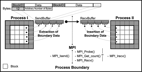
Figure 4: Design for parallel simulations. In the Figure, the MPI communication from process I to process II is depicted. First, the data to be communicated is extracted with provided functions from each Block and stored in send buffers. For pure fluid flows only PDFs have to be sent. On the sending side an MPI_Isend is scheduled and on the receiving side the message is either received with a MPI_Probe, MPI_GetCount and a MPI_Recv, or a MPI_Irecv. Note, that we attach a header to each Block message containing the BlockID and a communication direction. This is required in order to determine the Block to which the data has to be copied on the receiving side.

The parallelization of WaLBerla, which is depicted in Fig. 4, can be broken down into three steps: a data extraction step, a MPI communication step and a data insertion step. During the data extraction step, the data that has to be communicated is copied from the simulation data structures of the corresponding Blocks. Therefore, we distinguish between process-local and MPI communication for Blocks lying on the same or different processes. Local communication directly copies from the sending Block to the receiving Block, whereas for the MPI communication the data has first to be copied into buffers. For each process to which data has to be sent, one buffer is allocated. With the buffers, all messages from Blocks (block message) on the same process to another process are serialized. Additionally, the buffers are of data type byte and thus the MPI messages can contain any data type that can be converted into bytes. To extract the data to be communicated from the simulation data, extraction function objects are used. For each communication step and for each simulation data type several possible function objects are provided during the configuration of the communication. These are again selected via the functionality management. During the MPI communication one MPI message is sent to each process waiting for data from the current process. Therefore, nonblocking MPI functions are used, if the message size can be determined a priori. The data insertion step is similar to the data extraction, only here we traverse the block messages in the communication buffers instead of the Blocks.

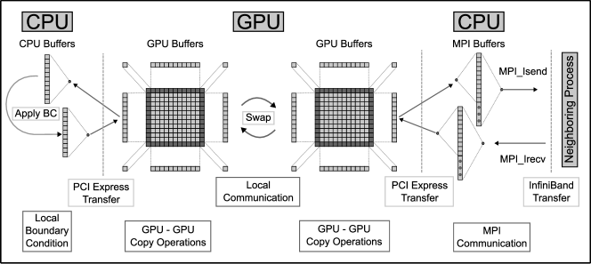
Figure 5: Multi-GPU design.

4.4 Multi GPU Implementation

For parallel GPU simulations part of the data stored on the GPU has to be transferred to the CPU via PCIe transfers before it can be communicated by means of the MPI communication. An efficient implementation of this transfer is important in order to sustain a large portion of the kernel performance. Hence, we only transfer the minimum amount of data necessary, the boundary values of the PDFs. Our parallel GPU implementation is depicted in Fig. 5 for one process having two Blocks. It can be seen that we extended the data structures by additional buffers on the GPU and on the CPU side. In $3$D, we add $6$ planes and $12$ edge buffers. To update the ghost layer of the PDFs and to prepare the GPU buffers for the MPI communication additional on-GPU copy operations are needed. The data of the buffers is copied to the ghost layer of the Blocks before the kernel call and the PDF boundary values of the PDF data are copied into the GPU buffers afterwards. For parallel simulations, the MPI implementation of Sec. 4.3 is used. Here, the only difference to the CPU implementation are the extraction and insertion functions, which for the local communication simply swap the GPU buffers, whereas the function cudaMemcpy is used to copy the data directly from the GPU buffers into the MPI buffers and vice versa for the MPI communication. To treat the boundary conditions at the domain boundary, the corresponding GPU buffers are transferred via cudaMemcpy to the CPU buffers. Next, the boundary conditions are applied and the data is copied back into the GPU buffers. The boundary conditions are fulfilled before the on-GPU copy operations.

4.5 Heterogeneous GPU / CPU Implementation

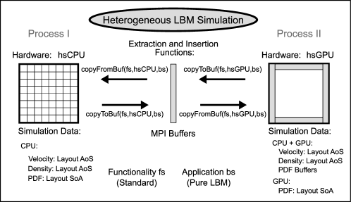
Figure 6: Heterogeneous simulation on GPU and CPU. The illustrated simulation is executed on two processes each having one Block covering half of the simulation domain. A standard LBM simulation is chosen as fs and on all Blocks the bs pure LBM is activated. Further, the first process runs on a CPU (hsCPU), whereas the second uses a GPU (hsGPU). According to these UIDs, the simulation data is allocated and the kernels, the extraction and insertion functions are selected. For the communication, extraction functions copyToBuf are selected by the UIDs of the corresponding Block to copy the communicated data in the specified format into the MPI send buffers. After the MPI communication, the insertion functions copyFromBuf copy the data from the MPI buffers back into the receiving data structures.

For parallel heterogeneous simulations, the information which Block runs on which hardware has to be known on all processes in our implementation. Hence, during the initialization we set on each process the hs of all Blocks to the hs of the process on which they are allocated. To determine the hs of each process, the input for the simulation describes all possible node configurations and a list which node belongs to which configuration. A node configuration defines how many processes can be executed on a particular node and which hs should be used for each process. Using these hardware selectors, it is now possible to utilize different LBM kernels and simulation data on different compute architectures. Further, all compute platforms use an identical layout for the MPI buffers, which acts as an interface for the MPI communication. Hence, the data in the MPI buffers is independent of the underlying hardware. During the MPI parallelization, only the extraction and insertion function have to be selected according to the hs of the Blocks to extract and insert the data from the different simulation data structures. Fig. 6 illustrates this in detail with a heterogeneous LBM simulation.

5 Investigation of Performance and Scalability

Subsequently, the performance of our design is discussed by means of Lid Driven Cavity scenarios in $3D$. In contrast to other highly optimized implementations on GPUs all measurements presented involve the PCIe data transfer of the complete halo layer from CPU to GPU and vice versa in each time step. Therefore, the actual performance is lower in contrast to [1] and [2]. However, scalability will be rather stable as most of the PCIe communication time is already accounted for by the single GPU simulation.

First of all, we investigate the single GPU and CPU performance including a detailed examination of the overhead for multi-GPU simulations in Sec. 7. Additionally, the overhead introduced by several Blocks per process is evaluated to estimate the suitability of the Patch and Block data structure for load balancing strategies. In Sec. 5.2 we conduct weak and strong scaling experiments in order to determine how the GPU implementation scales, on the HPC clusters introduced in Sec. 2.2. Finally, we investigate the performance of our design for heterogeneous computations in Sec. 5.3.

5.1 Single GPU and CPU Performance

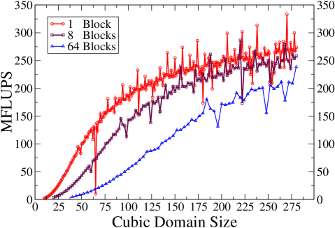
(a)

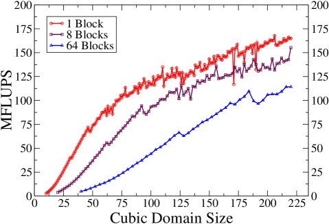
(b)

Figure 7: Single-GPU measurements on TinyGPU (TESLA C1060) for single (SP) and double precision (DP). A three dimensional partitioning is used to divide the simulation domain into Blocks. For a domain size of e.g. $200^{3}$ lattice cells and $64$ Blocks, each Block has a size of $50^{3}$ lattice cells.

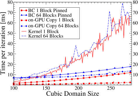
(a)

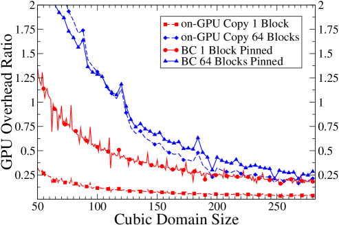
(b)

Figure 8: Single-GPU time measurements on TinyGPU(TESLA C1060) in SP. Fig. (a) shows the runtimes of different parts of the algorithm and Fig. (b) shows the ratio of the times for on-GPU copy operations and boundary condition handling (BC) to the kernel execution time. In both Figures results are given for $1$ and $64$ Blocks. Pinned memory denotes host memory allocated by the CUDA call cudaHostAlloc.

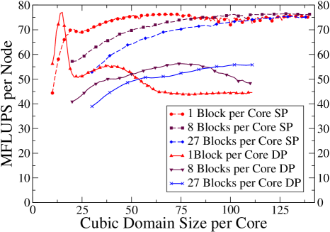
(a)

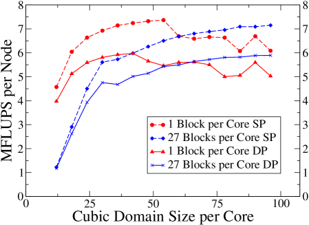
(b)

Figure 9: Single node CPU measurements on JUROPA (Xeon X5570) and JUGENE (BlueGene/P) for different Block numbers per core. For JUROPA $8$ and for JUGENE $4$ cores are used.

Our performance results for a single GPU having $1$ to $64$ local Blocks are depicted in Fig. 7. The performance increases with the domain size and saturates at a domain size of around $200^{3}$ lattice cells for a single Block. This is in contrast to the pure kernel measurements of Fig. 2, where the maximum performance is already reached for a domain size of around $70^{3}$ lattice cells. Fig. 8 shows that this results from the additional overhead of the on-GPU and BC copy operations. The same holds for the drop in performance using several Blocks, as the pure kernel runtime of $1$ and $64$ Blocks is nearly identical. For large domain sizes we loose about $5$ % for $8$ Blocks and $25$ % for $64$ Blocks compared to the runtime of one Block. Hence, if several small Blocks are required, e.g. for load balancing strategies, the performance of our GPU implementation will be reduced. The maximum achieved performance is $340$ (SP) / $167$ (DP) MFLUPS. Compared to the pure kernel performance we sustain around $80$ % using large domains for both SP and DP. For small domain sizes, e.g. $100^{3}$ lattice cells, we estimated in Tab. 1 a drop in performance from around $300$ to $264$ MFLUPS (SP), taking only the PCIe transfer into account. The measurements in Fig. 7 show a performance of around $190$ MFLUPS. As can be seen in Fig. 8, this discrepancy again results from the, in this case dominating, overheads of the on-GPU copies and the BC treatment. This clearly indicates that the PCIe transfer, which is included in the BC treatment, is not the only component crucial to sustain a large portion of the kernel performance. The on-GPU copy operations are hereby unavoidable, but the BC could be treated directly on the GPUs for further performance improvement. This will be investigated in future work.

The single node performance on JUROPA and JUGENE is presented in Fig. 9. Compared to the maximum single GPU performance the CPU performance corresponds to about $25$ % in SP and $33$ % in DP on JUROPA and $2$ % in SP and $3.5$ % in DP on JUGENE. Usually, we use domain sizes ranging from $90^{3}$ to $130^{3}$ in DP on one CPU core. For these sizes, the CPU measurements show a superior performance for multi-Block simulations compared to single Block simulations. This is in contrast to the GPU implementation, where multiple Blocks cause a degradation in performance. This results from an efficient utilization of the cache due to blocking effects occurring especially for the AoS data layout. Hence, for the investigated architectures block-structured grids are well suited for load balancing strategies.

5.2 Multi-CPU and GPU Performance

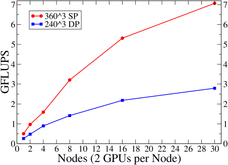
(a)

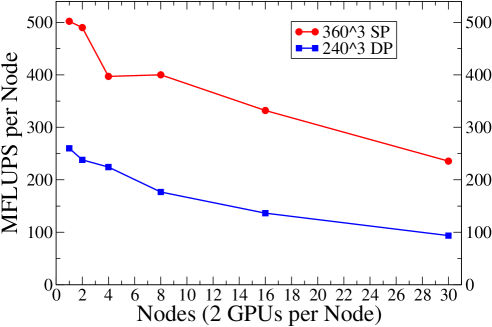
(b)

Figure 10: Multi-GPU strong scaling experiments on the NEC Nehalem cluster (TESLA S1070) with a domain size of $360^{3}$ lattice cells in SP and $240^{3}$ lattice cells in DP. The block decomposition is three dimensional. Figure (a) shows the absolute performance values, whereas Figure (b) shows the relative performance, i.e. the absolute performance divided by the number of compute nodes.

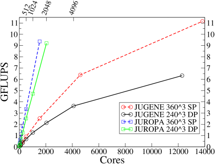
(a)

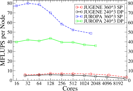
(b)

Figure 11: Multi-CPU strong scaling performance on JUROPA (Xeon X5570) and JUGENE (BlueGene/P). The block decomposition is three dimensional.

There are two basic scenarios to investigate parallel performance: weak scaling and strong scaling. In weak scaling experiments, the work load per compute node is kept constant for an increasing number of nodes. With this scenario the scalability and the overall manageable parallelism of the code is evaluated. Strong scaling experiments answer the question how much the time to solution can be reduced for a given problem. Therefore, the work load of all nodes is kept constant leading to a dominating communication overhead and thus a drop in speedup with an increasing number of nodes. An important point for the scalability of multi-GPU simulations is whether the performance scales if using two GPUs on the same node. On TinyGPU and the NEC Nehalem cluster this has been the case, as we achieved around $95$ % parallel efficiency for two GPUs. Further, weak scaling experiments on the NEC Nehalem cluster showed a nearly linear scaling up to $60$ GPUs for the domain size $222^{3}$ resulting in a maximum performance of around $16$ GFLUPS in SP. In comparison to todays CPUs, single GPUs offer a superior performance. Hence, on the one hand they should be well suited to reduce the time to solution in parallel simulations as less internode parallelism is required. On the other hand, the multi-GPU performance is not only hampered by the MPI communication, but also by the PCIe transfers, the on-GPU copies, and, in contrast to the CPU, the missing cache effect for small domains. In our GPU strong scaling experiments, depicted in Fig. 10, it can be seen that the relative performance for $1$ to $30$ compute nodes drops from around $500$ to $235$ MFLUPS in SP and from around $250$ to $100$ MFLUPS in DP. Compared to the CPU strong scaling experiments in Fig. 11, we need around $6$ (SP & DP) compute nodes on JUROPA and $75$ (SP) / $50$ (DP) on JUGENE to achieve the performance of a single GPU node on the NEC Nehalem cluster. To achieve the performance of $30$ GPU compute nodes, we need around $137$ (SP) / $70$ (DP) compute nodes on JUROPA and $1275$ (SP) / $750$ (DP) on JUGENE. The corresponding parallel efficiencies are: $46$ (SP) / $37$ (DP) % for the GPU implementation on NEC Nehalem cluster, $65$ (SP) / $93$ (DP) % for the CPU implementation on JUROPA and $90$ (SP) / $98$ (DP) % on JUGENE. Hence, to achieve the same time to solution our GPU implementation makes less efficient use of the utilized hardware, but also requires fewer nodes.

5.3 Heterogeneous GPU–CPU Performance

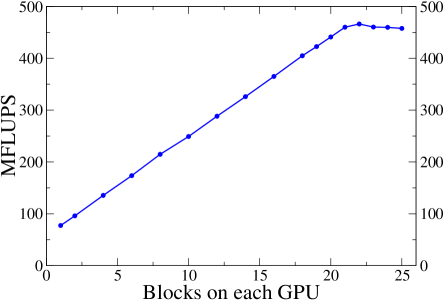
(a) Investigation of the load balance with 6 CPU-only processes each working on one Block and $2$ GPU processes with varying block counts. The Block size is $90^{3}$ lattice cells.

Block Size	$70^{3}$	$71^{3}$	$90^{3}$	$91^{3}$
Blocks	44	44	50	50
Processes
2 x GPU	379.1	341.6	422.6	404.3
2 x GPU + 6 x CPU	423.2	382.6	466.7	446.1
Block Size	$70^{3}$	$71^{3}$	$90^{3}$	$91^{3}$
Processes
6 x CPU (6 Blocks)	58.5	58.6	58.1	58.1
2 x GPU (2 Blocks)	388.2	431.2	495.3	469.2

(b) Performance comparison between homogeneous and heterogeneous setups depending on the Block size.

Figure 12: Heterogeneous performance on one compute node of TinyGPU (TESLA C1060) in SP.

To discuss the capabilities of heterogeneous simulations on GPUs and CPUs we first investigate the performance on a single compute node of TinyGPU. Here, best performance results are achieved with $6$ CPU only processes and $2$ for the GPUs. Additionally, the work load for each process has to be adjusted. This is depicted in Fig. 12(a), where each CPU process has one Block with $90^{3}$ lattice cells, whereas the number of blocks allocated on each GPU process is increased until the work load is balanced. Note that in the load-balanced case of $22$ Blocks on each GPU, the runtime of the GPU kernel is still $33$ % lower than the runtime of the CPU kernel, as on the GPU side a larger communication overhead is added to overall runtime. Further, in Tab. 12(b) the node performance of heterogeneous simulations is compared to simulations using only GPUs having the same number of Blocks or just one Block on each GPU. Hereby, the number of Blocks is chosen so that the heterogeneous simulations are load balanced. It can be seen that the heterogeneous simulations yield an increase in performance of around $42$ MFLUPS for all Block sizes, whereas the maximum for $6$ CPU processes would be around $58$ MFLUPS. Compared to simulations running on two GPU processes, which have only one Block on each process we loose around $5-12$ % performance due to the increased overhead. For the $70^{3}$ Block size the kernel performance is overly high due to padding effects and hence we gain around $10$ % in performance. Summarizing, for the mere purpose of a performance increase our current heterogeneous implementation is not suitable, but for simulations requiring several blocks on each process, e.g. for load balancing strategies or other optimizations, it is possible to improve the performance. Additionally, with our implementation the memory of GPU and CPU can be utilized, which allows for larger simulation setups. So far, we have only considered heterogeneous simulations on a single compute node. In Tab. 2 weak scaling experiments up to $90$ compute nodes are depicted. The weak scaling experiment using $60$ GPUs on $30$ compute nodes shows a perfect parallel efficiency and the heterogeneous experiment running on $60$ GPUs and $180$ CPU only processes has a parallel efficiency of $96$ %. In addition, we have conducted scaling experiments using different kind of compute nodes, e.g. compute nodes having only a CPU and nodes having additional GPUs. It can be seen that the performance scales well from $30$ up to $90$ compute nodes. Hence, with our implementation it is possible to efficiently utilize all nodes on clusters having heterogeneous node configurations. A further improvement of our heterogeneous design for multiphysics simulations could be the simulation of complex spatially contained functionality, e.g. a rising bubble, on processes running on CPUs and to only simulate pure fluid regions on the GPUs, for which they are currently suited best.

Blocks	GPU: $1$			GPU: $22$, CPU: $1$
Nodes	1	30		1	30	60	90
Processes	2 x GPU	60 x GPU		2 x GPU +	60 x GPU +	60 GPU +	60 GPU +
				6 x CPU	180 x CPU	420 x CPU	660 x CPU
MFLUPS	476	14480		459	13267	15684	17846

Table 2: Heterogeneous weak scaling experiments using up to $90$ compute nodes on the NEC Nehalem cluster. The simulation domain for nodes with GPUs is $90x4500x90$ and for CPU-only nodes $90x540x90$. All presented results are in SP and the load for the heterogeneous simulations is balanced.

6 Conclusion

A fundamental requirement for the utilization of GPUs in HPC clusters are scalable multi-GPU implementations. In this article, we have shown that this is possible for the LBM. Additionally, by means of our Patch and Block design, and our functionality management we have presented an approach for heterogeneous simulation on clusters equipped with varying node configurations. Further, we have shown that with our WaLBerla framework good runtime performance results can be achieved on various compute platforms despite the overhead for flexibility and its suitability for multiphysics simulations. In future work, we will optimize the memory accesses of our GPU implementation with the help of padding strategies as well as implement arbitrary boundary conditions, directly computed on the GPU. We will also investigate hybrid OpenMP and MPI parallelization in combination with heterogeneous simulations.

References

- [1] J. Tölke, M. Krafczyk, Teraflop Computing on a Desktop PC with GPUs for 3D CFD, Int. J. Comput. Fluid Dyn. 22 (7) (2008) 443–456.
- [2] J. Habich, T. Zeiser, G. Hager, G. Wellein, Speeding up a Lattice Boltzmann Kernel on nVIDIA GPUs, in: Proceedings of the First International Conference on Parallel, Distributed and Grid Computing for Engineering, Civil-Comp Press, 2009, p. 17.
- [3] C. Obrecht, F. Kuznik, B. Tourancheau, J.-J. Roux, A New Approach to the Lattice Boltzmann Method for Graphics Processing Units, Computers & Mathematics with Applications In Press, Corrected Proof.
- [4] M. Bernaschi, M. Fatica, S. Melchionna, S. Succi, E. Kaxiras, A Flexible High-Performance Lattice Boltzmann GPU Code for the Simulations of Fluid Flows in Complex Geometries, Concurrency and Computation: Practice and Experience 22 (1) (2010) 1–14.
- [5] TOP500 Supercomputer Sites, http://www.top500.org/ (Mar. 2010).
- [6] S. Chen, G. D. Doolen, Lattice Boltzmann Method for Fluid Flows, Annual Review of Fluid Mechanics 30 (1) (1998) 329–364.
- [7] S. Succi, The Lattice Boltzmann Equation for Fluid Dynamics and Beyond (Numerical Mathematics and Scientific Computation), Oxford University Press, USA, 2001.
- [8] X. He, L.-S. Luo, Lattice Boltzmann Model for the Incompressible Navier–Stokes Equation, Stat. Phys. 88 (3-4) (1997) 927–944.
- [9] T. Zeiser, G. Hager, G. Wellein, Benchmark Analysis and Application Results for Lattice Boltzmann Simulations on NEC SX Vector and Intel Nehalem Systems, Parallel Processing Letters 19 (4) (2009) 491–511.
- [10] C. K. Aidun, J. R. Clausen, Lattice-Boltzmann Method for Complex Flows, Annual Review of Fluid Mechanics 42 (1) (2010) 439–472.
- [11] C. Feichtinger, J. Götz, S. Donath, K. Iglberger, U. Rüde, WaLBerla: Exploiting Massively Parallel Systems for Lattice Boltzmann Simulations, in: R. Trobec, M. Vajtersic, P. Zinterhof (Eds.), Parallel Computing. Numerics, Applications, and Trends, Springer-Verlag, Berlin, Heidelberg, New York, 2009, pp. 240–259.
- [12] Regionales Rechenzentrum Erlangen, http://www.rrze.de/dienste/arbeiten-rechnen/hpc/systeme/tinygpu-cluster%.shtml (May 2010).
- [13] JUROPA Cluster Forschungszentrum Jülich, http://www.fz-juelich.de/portal/forschung/information/supercomputer/jur%opa (May 2010).
- [14] NEC Nehalem Cluster Höchstleistungsrechenzentrum Stuttgart, http://www.hlrs.de/systems/platforms/nec-nehalem-cluster/ (May 2010).
- [15] JUGENE Cluster Forschungszentrum Jülich, http://www.fz-juelich.de/portal/forschung/information/supercomputer/jug%ene (May 2010).
- [16] nVIDIA Cuda Toolkit 2.3, http://www.nvidia.com/object/cuda_get.html (Sep. 2009).
- [17] nVIDIA Cuda Programming Guide 2.3.1, http://developer.download.nvidia.com/compute/cuda/2_3/toolkit/docs/NVID%IA_CUDA_Programming_Guide_2.3.pdf (Aug. 2009).
- [18] Intel MPI Benchmarks, http://software.intel.com/en-us/articles/intel-mpi-benchmarks/ (May 2010).
- [19] The Stream Benchmark, http://www.streambench.org/ (Mar. 2010).
- [20] G. Wellein, T. Zeiser, G. Hager, S. Donath, On the Single Processor Performance of Simple Lattice Boltzmann Kernels, Computers & Fluids 35 (8-9) (2006) 910–919.
- [21] B. Boehm, A Spiral Model of Software Development and Enhancement, ACM SIGSOFT Software Engineering Notes 11 (4) (1986) 14–24.
- [22] H. van Vliet, Software Engineering: Principles and Practice, 3rd Edition, John Wiley & Sons, Inc. New York, NY, USA, 2008.
- [23] E. Gamma, R. Helm, R. Johnson, J. Vlissides, Design Patterns: Elements of Reusable Object-Oriented Software, Addison-Wesley Longman Publishing Co., Inc. Boston, MA, USA, 1995.
- [24] S. Donath, C. Feichtinger, T. Pohl, J. Götz, U. Rüde, Localized Parallel Algorithm for Bubble Coalescence in Free Surface Lattice-Boltzmann Method, in: Lecture Notes in Computer Science, Euro-Par 2009, Vol. 5704, Springer, 2009, pp. 735–746.
-
[25]
S. Bogner,
Simulation of Floating Objects in Free-Surface Flow,
Diploma Thesis (2009).
URL http://www10.informatik.uni-erlangen.de/Publications/Th%eses/2009/Bogner_DA09.pdf -
[26]
D. Haspel,
Simulation of Clotting Processes using Non-Newtonian Blood Models
and the Lattice Boltzmann Method, Master’s Thesis (2009).
URL http://www10.informatik.uni-erlangen.de/Publications/Th%eses/2009/Haspel_MA09.pdf - [27] J. Götz, K. Iglberger, C. Feichtinger, S. Donath, U. Rüde, Coupling Multibody Dynamics and Computational Fluid Dynamics on 8192 Processor Cores, Parallel Computing 36 (2-3) (2010) 142 – 151.
- [28] B. Dünweg, U. Schiller, A. J. C. Ladd, Statistical Mechanics of the Fluctuating Lattice Boltzmann Equation, Phys. Rev. E 76 (3) (2007) 036704.
- [29] H. Köstler, A Multigrid Framework for Variational Approaches in Medical Image Processing and Computer Vision, Verlag Dr. Hut, München, 2008.