Diffractive exclusive production of heavy quark pairs at high energy proton-proton collisions

Abstract:

We discuss exclusive double diffractive (EDD) production of heavy quark - heavy antiquark pairs at high energies. Differential distributions for $c\bar{c}$ at $\sqrt{s}$ = 1.96 GeV and for $b\bar{b}$ at $\sqrt{s}$ = 14 TeV are shown and discussed. Irreducible leading-order $b\bar{b}$ background to Higgs production is calculated for the first time in several kinematical variables. The signal-to-background ratio is shown and several improvements are suggested.

1 Introduction

There is recently a growing theoretical interest in studying exclusive processes. Exclusive production of the Higgs boson is a flag process of special interest and importance. Only a few processes have been measured so far at the Tevatron (see [1] and references therein). Khoze, Martin and Ryskin developed an approach in the language of off-diagonal unintegrated gluon distributions. This approach was applied to exclusive production of Higgs boson [2]. In our recent paper we applied the formalism to exclusive production of $c\bar{c}$ quarks. Quite large cross sections have been found [3].

The cross section for the Standard Model Higgs production is of the order of 1 fb for $M_{H}$ = 120 GeV [2]. The dominant $b\bar{b}$ decay channel is therefore preferential from the point of view of statistics. The $b\bar{b}$ exclusive production was estimated only at higher order [4]. It was argued that the leading-order contribution is rather small using a so-called $J_{z}$ = 0 rule [4]. Here we show a quantitative calculation which goes beyond this simple rule. In our calculation we include exact matrix element for massive quarks and the 2 $\to$ 4 phase space. This fully four-body calculation allows to impose cuts on any kinematical variable one wish to select. Different types of backgrounds to Higgs production were studied before e.g. in Ref.[5].

2 Formalism

2.1 The amplitude for $pp\to ppQ\bar{Q}$

Let us concentrate on the simplest case of the production of $q\bar{q}$ pair in the color singlet state. Color octet state would demand an emission of an extra gluon [4] which considerably complicates the calculations. We do not consider the $q\bar{q}g$ contribution as it is higher order compared to the one considered here.

In analogy to the Khoze-Martin-Ryskin approach (KMR) [2] for Higgs boson production, we write the amplitude of the exclusive diffractive $q\bar{q}$ pair production $pp\to p(q\bar{q})p$ in the color singlet state as

$${\cal M}_{\lambda_{q}\lambda_{\bar{q}}}^{pp\to ppq\bar{q}}(p^{\prime}_{1},p^{\prime}_{2},k_{1},k_{2}) = s\cdot\pi^{2}\frac{1}{2}\frac{\delta_{c_{1}c_{2}}}{N_{c}^{2}-1}\,\Im\int d^{2}q_{0,t}\;V_{\lambda_{q}\lambda_{\bar{q}}}^{c_{1}c_{2}}(q_{1},q_{2},k_{1},k_{2})$$ (1)

$$\frac{f^{\mathrm{off}}_{g,1}(x_{1},x_{1}^{\prime},q_{0,t}^{2},q_{1,t}^{2},t_{1})\;f^{\mathrm{off}}_{g,2}(x_{2},x_{2}^{\prime},q_{0,t}^{2},q_{2,t}^{2},t_{2})}{q_{0,t}^{2}\,q_{1,t}^{2}\,q_{2,t}^{2}}\;,$$

where $\lambda_{q},\,\lambda_{\bar{q}}$ are helicities of heavy $q$ and $\bar{q}$, respectively. Above $f_{1}^{\mathrm{off}}$ and $f_{2}^{\mathrm{off}}$ are the off-diagonal unintegrated gluon distributions in nucleon 1 and 2, respectively.

The longitudinal momentum fractions of active gluons are calculated based on kinematical variables of outgoing quark and antiquark: $x_{1}=\frac{m_{3,t}}{\sqrt{s}}\exp(+y_{3})+\frac{m_{4,t}}{\sqrt{s}}\exp(+y_{4})$ and $x_{2}=\frac{m_{3,t}}{\sqrt{s}}\exp(-y_{3})+\frac{m_{4,t}}{\sqrt{s}}\exp(-y_{4})$, where $m_{3,t}$ and $m_{4,t}$ are transverse masses of the quark and antiquark, respectively, and $y_{3}$ and $y_{4}$ are corresponding rapidities.

The bare amplitude above is subjected to absorption corrections. The absorption corrections are taken here in a simple multiplicative form.

2.2 $gg\to Q\bar{Q}$ vertex

Let us consider the subprocess amplitude for the $q\bar{q}$ pair production via off-shell gluon-gluon fusion. The vertex factor $V_{\lambda_{q}\lambda_{\bar{q}}}^{c_{1}c_{2}}=V_{\lambda_{q}\lambda_{\bar{q}}}^{c_{1}c_{2}}(q_{1},q_{2},k_{1},k_{2})$ in expression (1) is the production amplitude of a pair of massive quark $q$ and antiquark $\bar{q}$ with helicities $\lambda_{q}$, $\lambda_{\bar{q}}$ and momenta $k_{1}$, $k_{2}$, respectively. The color singlet $q\bar{q}$ pair production amplitude can be written as

$$V_{\lambda_{q}\lambda_{\bar{q}}}^{c_{1}c_{2}}(q_{1},q_{2},k_{1},k_{2})\equiv n^{+}_{\mu}n^{-}_{\nu}V_{\lambda_{q}\lambda_{\bar{q}}}^{c_{1}c_{2},\,\mu\nu}(q_{1},q_{2},k_{1},k_{2}),$$ (2)

The tensorial part of the amplitude reads:

$${}V_{\lambda_{q}\lambda_{\bar{q}}}^{\mu\nu}(q_{1},q_{2},k_{1},k_{2})=g_{s}^{2}\,\bar{u}_{\lambda_{q}}(k_{1})\biggl{(}\gamma^{\nu}\frac{\hat{q}_{1}-\hat{k}_{1}-m}{(q_{1}-k_{1})^{2}-m^{2}}\gamma^{\mu}-\gamma^{\mu}\frac{\hat{q}_{1}-\hat{k}_{2}+m}{(q_{1}-k_{2})^{2}-m^{2}}\gamma^{\nu}\biggr{)}v_{\lambda_{\bar{q}}}(k_{2}).$$

(3)

The coupling constants $g_{s}^{2}\to g_{s}(\mu_{r,1}^{2})g_{s}(\mu_{r,2}^{2})$. In the present calculation we take the renormalization scale to be $\mu_{r,1}^{2}=\mu_{r,2}^{2}=M_{q\bar{q}}^{2}/4$ or $M_{q\bar{q}}^{2}$. The exact matrix element is calculated numerically.

2.3 Off-diagonal unintegrated gluon distributions

In the KMR approach the off-diagonal parton distributions (i=1,2) are calculated as

$$f_{i}^{\mathrm{KMR}}(x_{i},Q_{i,t}^{2},\mu^{2},t_{i}) = R_{g}\frac{d[g(x_{i},k_{t}^{2})S_{1/2}(k_{t}^{2},\mu^{2})]}{d\log k_{t}^{2}}|_{k_{t}^{2}=Q_{it}^{2}}\;F(t_{i})\;$$ (4)

$$\approx R_{g}\frac{dg(x_{i},k_{t}^{2})}{d\log k_{t}^{2}}|_{k_{t}^{2}=Q_{i,t}^{2}}\;S_{1/2}(Q_{i,t}^{2},\mu^{2})\;F(t_{i})\;,$$

where $S_{1/2}(q_{t}^{2},\mu^{2})$ is a Sudakov-like form factor relevant for the case under consideration. The last approximate equalities come from the fact that in the region under consideration the Sudakov-like form factors are somewhat slower functions of transverse momenta than the collinear gluon distributions. While reasonable for an estimate of gluon distribution it may be not sufficient for precise calculation of the cross section. It is reasonable to take a running (factorization) scale as: $\mu_{1}^{2}=\mu_{2}^{2}=M_{q\bar{q}}^{2}/4$ or $M_{q\bar{q}}^{2}$.

The factor $R_{g}$ here cannot be calculated from first principles in the most general case of off-diagonal UGDFs. It can be estimated in the case of off-diagonal collinear PDFs when $x^{\prime}\ll x$ and $xg=x^{-\lambda}(1-x)^{n}$. Then $R_{g}=\frac{2^{2\lambda+3}}{\sqrt{\pi}}\frac{\Gamma(\lambda+5/2)}{\Gamma(\lambda+4)}$. Typically $R_{g}\sim$ 1.3 – 1.4 at the Tevatron energy. The off-diagonal form factors are parametrized here as $F(t)=\exp\left(B_{\mathrm{off}}t\right)$. In practical calculations we take $B_{\mathrm{off}}$ = 2 GeV^-2. In the original KMR approach the following prescription for the effective transverse momentum is taken: $Q_{1,t}^{2}=\min\left(q_{0,t}^{2},q_{1,t}^{2}\right)$ and $Q_{2,t}^{2}=\min\left(q_{0,t}^{2},q_{2,t}^{2}\right)$. In evaluating $f_{1}$ and $f_{2}$ needed for calculating the amplitude (1) we use different collinear distributions. It was proposed [2] to express the $S_{1/2}$ form factors in Eq. (4) through the standard Sudakov form factors as:

$$S_{1/2}(q_{t}^{2},\mu^{2})=\sqrt{T_{g}(q_{t}^{2},\mu^{2})}\;.$$ (5)

2.4 Cross section

The cross section is calculated as

$$d\sigma=\frac{1}{2s}|{\cal M}_{2\to 4}|^{2}(2\pi)^{4}\delta^{4}(p_{a}+p_{b}-p_{1}-p_{2}-p_{3}-p_{4})\frac{d^{3}p_{1}}{(2\pi)^{3}2E_{1}}\frac{d^{3}p_{2}}{(2\pi)^{3}2E_{2}}\frac{d^{3}p_{3}}{(2\pi)^{3}2E_{3}}\frac{d^{3}p_{4}}{(2\pi)^{3}2E_{4}}\;.$$ (6)

The details how to conveniently reduce the number of kinematical integration variables are given elsewhere.

3 Results

3.1 $pp\to ppc\bar{c}$

Let us proceed now with the presentation of differential distributions of charm quarks produced in the EDD mechanism. In this case we have fixed the scale of the Sudakov form factor to be $\mu=M_{c\bar{c}}/2$. Such a choice of the scale leads to a strong damping of the cases with large rapidity gaps between $q$ and $\bar{q}$.

In the left panel of Fig. 1 we show distribution in rapidity. The results obtained with the KMR method are shown together with inclusive gluon-gluon contribution. The effect of absorption leads to a damping of the cross section by an energy-dependent factor. For the Tevatron this factor is about 0.1. If the extra factor is taken into account the EDD contribution is of the order of 1% of the dominant gluon-gluon fusion contribution.

The corresponding rapidity-integrated cross section at $\sqrt{s}$ = 1960 GeV is: 6.6 $\mu$b for the exact formula, 2.4 $\mu$b for the simplified formula (see Eq. (4)). For comparison the inclusive cross section (gluon-gluon component only) is 807 $\mu$b.

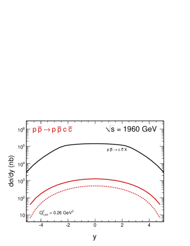
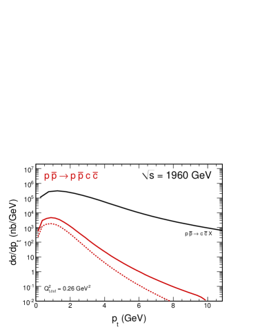
Figure 1: Rapidity distribution of $c$ or $\bar{c}$ (left) and transverse momentum distribution of $c$ or $\bar{c}$ (right). The top curve is for inclusive production in the $k_{t}$-factorization approach with the Kwieciński UGDF and $\mu^{2}=4m_{c}^{2}$, while the two lower lines are for the EDD mechanism for the KMR UGDF with leading-order collinear gluon distribution [11]. The solid line is calculated from the exact formula and the dashed line for the simplified formula (when only derivative of collinear GDF is taken). An extra cut on the momenta in the loop $Q_{t,cut}^{2}$ = 0.26 GeV² was imposed. Absorption effects were included approximately by multiplying the cross section by the gap survival factor $S_{G}$ = 0.1.

In the right panel of Fig. 1 we show the differential cross section in transverse momentum of the charm quark. Compared to the inclusive case, the exclusive contribution falls significantly faster with transverse momentum than in the inclusive case.

In Fig. 2 we show the distribution in the invariant mass of the $c$ $\bar{c}$ system. Compared to the inclusive case the invariant mass distribution for the EDD component is significantly steeper. This is due to the Sudakov-like form factor which, according to the procedure described above, damps the cross section for large invariant masses.

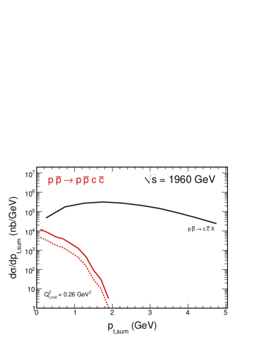
Figure 2: Invariant mass distribution of the $c\bar{c}$ pair (left) and distribution in the transverse momentum of the $c\bar{c}$ pair (right). The other details are the same as in the previous figure

As in the inclusive case within the $k_{t}$-factorisation approach the $c\bar{c}$ pair possesses the transverse momentum different from zero. The corresponding distribution is shown in the right panel of Fig. 2. The distribution for the exclusive case (the two lower lines) is much narrower compared to the inclusive case (the upper line).

3.2 $pp\to ppb\bar{b}$

In parallel to the exclusive $b\bar{b}$ production, we calculate the differential cross sections for exclusive Higgs boson production. Compared to the standard KMR approach here we calculate the amplitude with the hard subprocess $g^{*}g^{*}\to H$ taking into account off-shellness of the active gluons. The details of the off-shell matrix element can be found in Ref. [6]. In contrast to the exclusive $\chi_{c}$ production [7], due to a large factorization scale $\sim M_{H}$ the off-shell effects for $g^{*}g^{*}\to H$ give only a few percents to the final result.

The same unintegrated gluon distributions based on the collinear distributions are used for the Higgs and continuum $b{\bar{b}}$ production. In the case of exclusive Higgs production we calculate the four-dimensional distribution in the standard kinematical variables: $y,t_{1},t_{2}$ and $\phi$. Assuming the full coverage for outgoing protons we construct the two-dimensional distributions $d\sigma/dyd^{2}p_{t}$ in Higgs rapidity and transverse momentum. The distribution is used then in a simple Monte Carlo code which includes the Higgs boson decay into the $b{\bar{b}}$ channel. It is checked subsequently whether $b$ and $\bar{b}$ enter into the pseudorapidity region spanned by the central detector.

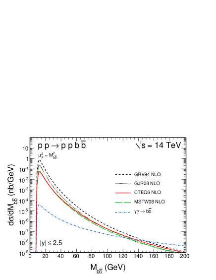
Figure 3: The $b\bar{b}$ invariant mass distribution for $\sqrt{s}$ = 14 TeV and for $-2.5<y<2.5$ corresponding to the ATLAS/CMS detectors. The absorption effects were taken into account by multiplying by the gap survival factor $S_{G}$ = 0.03.

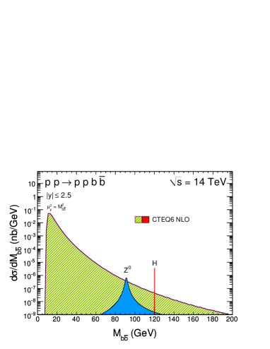
Figure 4: The $b\bar{b}$ invariant mass distribution for $\sqrt{s}$ = 14 TeV and for $b$ and $\bar{b}$ jets in the rapidity interval $-2.5<y<2.5$ corresponding to the ATLAS detector. The absorption effects for the Higgs boson and the background were taken into account by multiplying by the gap survival factor $S_{G}$ = 0.03. The left panel shows purely theoretical predictions, while the right panel includes experimental effects due to experimental uncertainty in invariant mass measurement.

In Fig. 3 we show the most essential distribution in the invariant mass of the centrally produced $b\bar{b}$ pair, which is also being the missing mass of the two outgoing protons. In this calculation we have taken into account typical detector limitations in rapidity $-2.5<y_{b},y_{\bar{b}}<2.5$. We show results with different collinear gluon distributions from the literature: GRV [11], CTEQ [12], GJR [13] and MSTW [14]. The results obtained with radiatively generated gluon distributions (GRV, GJR) allow to use low values of $Q_{t}=q_{0t},q_{1t},q_{2t}$ whereas for other gluon distributions an upper cut on $Q_{t}$ is necessary. The integrated double-diffractive $b\bar{b}$ contribution calculated here seems bigger than the contribution of the exclusive photoproduction of $b\bar{b}$ estimated in [15]. The lowest curve in Fig.3 represents the $\gamma\gamma$ contribution [8]. While the integrated over phase space $\gamma\gamma$ contribution is rather small, it is significant compared to the double-diffractive component at large $M_{b\bar{b}}>$ 100 GeV. This can be understood by a damping of the double diffractive component at large $M_{b\bar{b}}$ by the Sudakov form factor [2, 3]. In addition, in contrast to the double-diffractive component the absorption for the $\gamma\gamma$ component is very small and in practice can be neglected.

In the left panel of Fig.4 we show the double diffractive contribution for a selected (CTEQ6 [12]) collinear gluon distribution and the contribution from the decay of the Higgs boson including natural decay width calculated as in Ref. [16], see the sharp peak at $M_{b\bar{b}}$ = 120 GeV. The phase space integrated cross section for the Higgs production, including absorption effects with $S_{G}=0.03$ is somewhat less than 1 fb. The result shown in Fig.4 includes also the branching fraction for BR($H\to b\bar{b})\approx$ 0.8 and the rapidity restrictions. The second much broader Breit-Wigner type peak corresponds to the exclusive production of the $Z^{0}$ boson with the cross section calculated as in Ref. [17]. The exclusive cross section for $\sqrt{s}$ = 14 TeV is 16.61 fb including absorption. The branching fraction BR($Z^{0}\to b\bar{b})\approx$ 0.15 has been included in addition. In contrast to the Higgs case the absorption effects for the $Z^{0}$ production are much smaller [17]. The sharp peak corresponding to the Higgs boson clearly sticks above the background. In the above calculations we have assumed an ideal no-error measurement.

In reality the situation is, however, much worse as both protons and in particular $b$ and $\bar{b}$ jets are measured with a certain precision which automatically leads to a smearing in $M_{b\bar{b}}$ . Experimentally instead of $M_{b\bar{b}}$ one will measure rather two-proton missing mass ($M_{pp}$). The experimental effects are included in the simplest way by a convolution of the theoretical distributions with the Gaussian smearing function $G(M)=\frac{1}{\sqrt{2\pi}\sigma}\exp\left(\frac{(M-M_{H})^{2}}{2\sigma^{2}}\right)$ with $\sigma$ = 2 GeV [18, 19] which is determined mainly by the precision of measuring forward protons. In the right panel we show the two-proton missinging mass distribution when the smearing is included. Now the bump corresponding to the Higgs boson is below the $b\bar{b}$ background. With the experimental resolution assumed above the identification of the Standard Model Higgs seems rather difficult. The situation for some scenarios beyond the Standard Model may be better [20, 21].

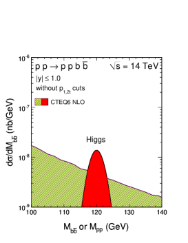
Figure 5: The $b\bar{b}$ invariant mass distribution for $\sqrt{s}$ = 14 TeV for a limited range of $b$ and $\bar{b}$ rapidities: $-1<y<1$.

Can the situation be improved by imposing further cuts? In Fig. 5 (left panel) we show the result for a more limited range of $b$ and $\bar{b}$ rapidity, i.e. not making use of the whole coverage of the main LHC detectors. Here we omit the $Z^{0}$ contribution and concentrate solely on the Higgs signal. Now the signal-to-background ratio is somewhat improved. This would be obviously at the expense of a deteriorated statistics. Similar improvements of the signal-to-background ratio can be obtained by imposing cuts on jet transverse momenta. Detailed studies of the role of cuts will be discussed in [9].

We are indebted to Valery Khoze, Misha Ryskin, Andy Pilkington and Christophe Royon for a discussion and exchange of useful information.

References

- [1] M.G. Albrow, T.D. Coughlin and J.R. Forshaw, Arxiv.1006.1289.
-
[2]
V. A. Khoze, A. D. Martin and M. G. Ryskin,
Phys. Lett. B 401, 330 (1997);
A. B. Kaidalov, V. A. Khoze, A. D. Martin and M. G. Ryskin, Eur. Phys. J. C 33, 261 (2004). - [3] R. Maciuła, R. Pasechnik and A. Szczurek, Phys. Lett. B 685, 165 (2010).
- [4] V. A. Khoze, M. G. Ryskin and A. D. Martin, Eur. Phys. J. C 64, 361 (2009).
- [5] M. Chaichian, P. Hoyer, K. Huitu, V.A. Khoze and A.D. Pilkington, JHEP 0905 (2009) 011.
- [6] R. S. Pasechnik, O. V. Teryaev and A. Szczurek, Eur. Phys. J. C 47, 429 (2006).
-
[7]
R. S. Pasechnik, A. Szczurek and O. V. Teryaev,
Phys. Rev. D 78, 014007 (2008);
R. S. Pasechnik, A. Szczurek and O. V. Teryaev, Phys. Lett. B 680, 62 (2009);
R. S. Pasechnik, A. Szczurek and O. V. Teryaev, Phys. Rev. D 81, 034024 (2010). - [8] R. Maciuła, R.S. Pasechnik and A. Szczurek, arXiv:1006.3007 (hep-ph).
- [9] R. Maciuła, R.S. Pasechnik and A. Szczurek, a work in preparation.
- [10] T.D. Coughlin and J.R. Forshaw, JHEP 1001, 121 (2010).
- [11] M. Glück, E. Reya and A. Vogt, Z. Phys. C67, 433 (1995).
- [12] J. Pumplin et al., JHEP 0207, 012 (2002).
- [13] M. Glück, D. Jimenez-Delgado, E. Reya, Eur. Phys. J. C53, 355 (2008).
- [14] A.D. Martin et al., Eur. Phys. J. C63, 189 (2009).
- [15] V.P. Goncalves and M.V.T. Machado, Phys. Rev. D75, 031502(R) (2007).
- [16] G. Passarino, Nucl. Phys. B 488, 3 (1997).
- [17] A. Cisek, W. Schäfer and A. Szczurek, Phys. Rev. D80 074013 (2009).
- [18] A. Pilkington, private communication.
- [19] Ch. Royon, private communication.
- [20] S. Heinemeyer, V.A. Khoze, M.G. Ryskin, W.J. Stirling, M. Tasevsky and G. Weiglein, Eur. Phys. J. C53 (2008) 231.
- [21] B.E. Cox, F.K. Loebinger and A.D. Pilkington, JHEP 0710, 090 (2007).
- [22] M. Boonekamp, R. Peschanski and C. Royon, Phys. Rev. Lett. 87 251806 (2001).