Anomalous tensor magnetic moments and form factors of the proton in the self-consistent chiral quark-soliton model

Abstract

We investigate the form factors of the chiral-odd nucleon matrix element of the tensor current. In particular, we aim at the anomalous tensor magnetic form factors of the nucleon within the framework of the SU(3) and SU(2) chiral quark-soliton model. We consider $1/N_{c}$ rotational corrections and linear effects of SU(3) symmetry breaking with the symmetry-conserving quantization employed. We first obtain the results of the anomalous tensor magnetic moments for the up and down quarks: $\kappa_{T}^{u}=3.56$ and $\kappa_{T}^{d}=1.83$, respectively. The strange anomalous tensor magnetic moment is yielded to be $\kappa_{T}^{s}=0.2\sim-0.2$, that is compatible with zero. We also calculate the corresponding form factors $\kappa_{T}^{q}(Q^{2})$ up to a momentum transfer $Q^{2}\leq 1\,\mathrm{GeV}^{2}$ at a renormalization scale of $0.36\,\mathrm{GeV}^{2}$.

I Introduction

The transversity of the nucleon is an important issue in hadron physics Ralston:1980pp ; Jaffe:1991ra ; Cortes:1991ja (see also the review review ; Boffi:review ), since, together with the helicity distribution, they are the leading-twist parton distributions with which one tries to understand the spin structure of the nucleon. However, it is of great difficulty to measure the transversity of the nucleon because it decouples from deep inelastic scattering due to its chiral-odd nature. Only very recently, information on the transversity of the nucleon is available from the transverse spin asymmetry $A_{TT}$ of Drell-Yan processes in $p\overline{p}$ reactions Efremov:2004 ; Anselimo:2004 ; PAX:2005 ; Pasquini:2006 as well as the azimuthal single spin asymmetry in semi-inclusive deep inelastic scattering (SIDIS) Anselmino:tensorcharge .

The chiral-odd nucleon matrix element is parameterized by three form factors Diehl:GPDhFlip ; Hagler:FFdecomposition which we denote as $H_{T}(Q^{2})$, $E_{T}(Q^{2})$ and $\tilde{H}_{T}(Q^{2})$. The first one was studied in Ref. Ledwig:2010tu together with the tensor charges within the SU(3) chiral quark-soliton model ($\chi$QSM). Beside the tensor charges HeJi:TensorCharges , also the linear combination $\kappa_{T}^{q}(0)=E_{T}^{q}(0)+2\tilde{H}_{T}^{q}(0)$ was found to be interesting. It was found that $\kappa_{T}^{q}$ is a more fundamental quantity DiehlHaegler:ATMM than $E_{T}^{q}$ and $\tilde{H}_{T}^{q}$ by themselves and describes the transverse deformation of the transverse polarized quark distribution in an unpolarized nucleon. Burkardt Burkardt:2005 investigated the connection of the quantity $\kappa_{T}^{q}$ to the Boer-Mulders function $h_{1}^{\perp q}$ BoerMulders:1998 and presented the relation

$$h_{1}^{\perp q}\sim-\kappa_{T}^{q}\,\,\,,$$ (1)

which is similar to the relation of the Sivers-function $f_{1T}^{\perp q}$ Sivers:1991 to the anomalous magnetic moment $\kappa^{q}$, i.e. $f_{1T}^{\perp q}\sim-\kappa^{q}$ Burkardt:2004a ; Burkardt:2004b ; Burkardt:2004c . The latter relation is confirmed by the HERMES collaboration HERMES:2005 . The Boer-Mulders function $h_{1}^{\perp q}$ represents the asymmetry of the transverse momentum of quarks perpendicular to the quark spin in an unpolarized nucleon, while the Sivers function explains the transverse momentum asymmetry of quarks in a transversely polarized target. Both the Sivers- and Boer-Mulders functions contribute to SIDIS processes and a measurement of $h_{1}^{\perp q}$ can provide information on the anomalous tensor magnetic moment $\kappa_{T}^{q}$ Burkardt:2006 . However, it is very hard to measure chiral-odd observables. So far, only the transversity distribution $\delta q(x)$ was extracted Anselmino:tensorcharge , based on a global analysis of the data of the azimuthal single spin asymmetry in SIDIS processes $lp^{\uparrow}\to l\pi X$ by the Belle Belle:2006 , HERMES HERMES:2005 ; HERMES:2006 and COMPASS COMPASS:2007 collaborations. The corresponding tensor charges were obtained as $\delta u=0.54_{-0.22}^{+0.09}$ and $\delta d=-0.23_{-0.16}^{+0.09}$ at a scale of $\mu^{2}=0.8\,\,\mbox{GeV}^{2}$ Anselmino:2009 .

In the present work, we aim at investigating the anomalous tensor magnetic form factors of the nucleon and extend our previous study on the nucleon tensor form factors Ledwig:2010tu . The anomalous tensor magnetic moment is interpreted as a quantity that describes how the average position of quarks with spin in the $x$-direction is shifted to the $y$-direction for an unpolarized target relative to the transverse center of the momentum Burkardt:2005 . Some amount of theoretical works on the anomalous tensor magnetic moment was already performed, for example, in light-cone constituent quark models Paspquini:2005 ; Paspquini:2007 , on the lattice Hagler:2008 , in the SU(2) $\chi$QSM Wakamatsu:2008 and estimations given in Ref. Burkardt:2008 . Presently all the results indicate positive values of the anomalous tensor magnetic moment for the up and down quarks, i.e. $\kappa_{T}^{u}>0$ and $\kappa_{T}^{d}>0$.

We will use the self-consistent SU(3) and SU(2) chiral quark-soliton model ($\chi$QSM) Christov:1995vm in order to compute the anomalous tensor magnetic moments. The $\chi$QSM is an effective chiral model for QCD in the low-energy regime, consisting of constituent quarks and the pseudo-scalar mesons as the relevant degrees of freedom. Originally, the $\chi$QSM was developed based on the QCD instanton vacuum Diakonov:1987ty ; CQSM:Diakonovlecture and has only a few free parameters. These parameters can mostly be fixed to the meson masses and decay constants in the mesonic sector. The only free parameter in the baryon sector is the constituent quark mass that is fixed by reproducing the nucleon electric charge radius. Hence, all other baryon observables are obtained in exactly the same framework without adjusting further parameters. In the past, the model was very successful in describing basically all baryon observablesChristov:1995vm . Furthermore, the renormalization scale for the $\chi$QSM is naturally given by the cut-off parameter for the regularization which is about $0.36\,\mathrm{GeV^{2}}$. Note that it is implicitly related to the inverse of the size of instantons ($\overline{\rho}\approx 0.35\,\mathrm{fm}$) Diakonov:1983hh ; Diakonov:1985eg . It plays in particular an important role in investigating the tensor charges and anomalous tensor magnetic moments of the nucleon, since they depend on the renormalization scale already at one-loop level.

We sketch the work as follows. In Section II we briefly explain how to derive the anomalous tensor magnetic moments within the framework of the $\chi$QSM. In Section III we present the results of this work. Section IV is devoted to conclusion and summary. The explicit expressions for the relevant densities can be found in the Appendix.

II Anomalous tensor magnetic form factors

We begin with the nucleon matrix element of the tensor quark current, which is parametrized in terms of three tensor form factors

$$\langle N(p^{\prime},\,s_{3}^{\prime})|\bar{\psi}(0)i\sigma_{\mu\nu}\lambda^{\chi}\psi(0)|N(p,\,s_{3})\rangle = \overline{u}(p^{\prime},s_{3}^{\prime})\left[H_{T}^{\chi}(Q^{2})i\sigma^{\mu\nu}+E_{T}^{\chi}(Q^{2})\frac{\gamma^{\mu}q^{\nu}-q^{\mu}\gamma^{\nu}}{2M}\right.$$ (3)

$$\hskip 28.45274pt\left.+\;\tilde{H}_{T}^{\chi}(Q^{2})\frac{(n^{\mu}q^{\nu}-q^{\mu}n^{\nu})}{2M^{2}}\right]u(p,\,s_{3}),$$

where $\sigma_{\mu\nu}$ is the spin operator $i[\gamma_{\mu},\,\gamma_{\nu}]/2$ and $\lambda^{\chi}$ the Gell-Mann matrices where we also include the unity by $\lambda^{0}=1$. The $\psi$ represents the quark field. The $u(p,\,s_{3})$ denotes the nucleon spinor of mass $M$ with momentum $p$ and the third component of the nucleon spin $s_{3}$. The momentum transfer $q$ and total momentum $n$ are defined as $q=p^{\prime}-p$ and $n=p^{\prime}+p$ respectively. The $Q^{2}$ is defined as $Q^{2}=-q^{2}$ with $Q^{2}>0$. In the previous work, we have already calculated the tensor form factor $H_{T}^{\chi}(Q^{2})$ within the same framework. We proceed in this work to the anomalous tensor magnetic form factor $\kappa_{T}^{\chi}(Q^{2})=E_{T}^{\chi}(Q^{2})+2\tilde{H}_{T}^{\chi}(Q^{2})$. In fact, it is technically rather complicated to consider the form factor $E_{T}^{\chi}(Q^{2})$ and also $\tilde{H}_{T}^{\chi}(Q^{2})$. However, we will see that in the linear combination $E_{T}^{\chi}(Q^{2})+2\tilde{H}_{T}^{\chi}(Q^{2})$ these difficulties drop out.

In order to extract $\kappa_{T}^{\chi}(Q^{2})$ from Eq. (3), we take the components $\mu=0$ and $\nu=k$ of the tensor current with $s_{3}^{\prime}=s_{3}=+1/2$ fixed and use the Breit frame. Multiplying the matrix element by $q^{k}$, we obtain

$$-\langle N(p^{\prime},\,\frac{1}{2})|\psi^{\dagger}\gamma^{k}\lambda^{\chi}\psi|N(p,\,\frac{1}{2})\rangle q^{k} = \frac{{\bm{q}}^{2}}{2M}\left(H_{T}^{\chi}(Q^{2})\;+\;E_{T}^{\chi}(Q^{2})\;+\;2\tilde{H}_{T}^{\chi}(Q^{2})\frac{E^{2}}{M^{2}}\right),$$ (4)

where $E=\sqrt{M^{2}+{\bm{q}}^{2}/4}$ is the on-shell energy of the nucleon. It is convenient to define a combined form factor $H_{T}^{*\chi}(Q^{2})$ as

$$H_{T}^{*\chi}(Q^{2})\;=\;\frac{2M}{{\bm{q}}^{2}}\int\frac{d\Omega}{4\pi}\langle N_{\frac{1}{2}}(p^{\prime})|\psi^{\dagger}\gamma^{k}q^{k}\lambda^{\chi}\psi|N_{\frac{1}{2}}(p)\rangle\,\,\,,$$ (5)

so that the third form factor $\tilde{H}_{T}^{\chi}(Q^{2})$ is expressed in terms of the other three form factors as follows:

$$2\tilde{H}_{T}^{\chi}(Q^{2})\frac{E^{2}}{M^{2}} = -H_{T}^{\chi}(Q^{2})-E_{T}^{\chi}(Q^{2})-H_{T}^{*\chi}(Q^{2})\,\,\,.$$ (6)

Inserting this in the definition $\kappa_{T}^{\chi}=E^{\chi}_{T}(0)+2\tilde{H}_{T}^{\chi}(0)$, we are able to reexpress the flavor-decomposed anomalous tensor magnetic moments as

$$\kappa_{T}^{\chi}=-H_{T}^{\chi}(0)-H_{T}^{*\chi}(0),$$ (7)

with $\chi=0,3,8$ and $\lambda^{0}=1$.

Thus, in the present work we aim at calculating Eq. (5) in the $\chi$QSM and combining it with the results for $H_{T}^{\chi}(Q^{2})$ in the previous work Ledwig:2010tu to determine the flavor-decomposed $\kappa_{T}^{q}(Q^{2})$ with $q=u,\,d,\,s$. Explicitly, they are expressed in SU(3) as

$$\kappa_{T}^{u} = \frac{1}{2}\left(\frac{2}{3}\kappa_{T}^{0}+\kappa_{T}^{3}+\frac{1}{\sqrt{3}}\kappa_{T}^{8}\right),$$ (8)

$$\kappa_{T}^{d} = \frac{1}{2}\left(\frac{2}{3}\kappa_{T}^{0}-\kappa_{T}^{3}+\frac{1}{\sqrt{3}}\kappa_{T}^{8}\right),$$ (9)

$$\kappa_{T}^{s} = \frac{1}{3}\left(\kappa_{T}^{0}-\sqrt{3}\kappa_{T}^{8}\right),$$ (10)

and in SU(2) with $\tau^{0}=1$ as:

$$\kappa_{T}^{u} = \frac{1}{2}\left(\kappa_{T}^{0}+\kappa_{T}^{3}\right),$$ (11)

$$\kappa_{T}^{d} = \frac{1}{2}\left(\kappa_{T}^{0}-\kappa_{T}^{3}\right).$$ (12)

In order to compare the present results for the form factors with those of other works, it is essential to know at which renormalization scale the calculation was carried out, since the tensor form factors depend on the renormalization scale already at one-loop level. Hence, we will use the following equation review ; Evolution1 in order to compare results obtained at different renormalization scales:

$$\kappa_{T}^{q}(\mu^{2}) = \left(\frac{\alpha_{S}(\mu^{2})}{\alpha_{S}(\mu_{i}^{2})}\right)^{4/27}\left[1-\frac{337}{486\pi}\left(\alpha_{S}(\mu_{i}^{2})-\alpha_{S}(\mu^{2})\right)\right]\kappa_{T}^{q}(\mu_{i}^{2})$$ (13)

$$\alpha_{S}^{NLO}(\mu^{2}) = \frac{4\pi}{9\ln(\mu^{2}/\Lambda^{2})}\left[1-\frac{64}{81}\frac{\ln\ln(\mu^{2}/\Lambda^{2})}{\ln(\mu^{2}/\Lambda^{2})}\right]$$ (14)

with $\Lambda=0.248$ GeV and $N_{c}=N_{f}=3$.

III Anomalous tensor magnetic form factors in the Chiral Quark-Soliton Model

Having performed a tedious but straightforward calculation following Refs. Kim:eleff ; Christov:1995vm ; Silva:Strange , we finally arrive at the complete expressions for the SU(3) form factors $H_{T}^{*\chi}(Q^{2})$ for the cases $\chi=3,8$ and $\chi=0$ as follows:

$$H_{T}^{*\chi}(Q^{2}) = \frac{2}{3}M\int dr\,\,r^{3}\,\left\{j_{0}(|\bm{Q}|r)+j_{2}(|\bm{Q}|r)\right\}\,\,\langle N^{\prime}|\mathcal{H}_{T}^{*\chi}(r)|N\rangle,$$ (15)

$$\mathcal{H}_{T}^{*\chi=3,8}(r) = -D_{\chi 8}^{(8)}\mathcal{Q}_{T0}(r)+\frac{1}{\sqrt{3}I_{1}}D_{\chi i}^{(8)}J_{i}\mathcal{X}_{T1}(r)+\frac{\sqrt{3}}{2I_{2}}D_{\chi a}J_{a}\,\mathcal{X}_{T2}(r)$$

$$-\frac{2}{\sqrt{3}}\frac{K_{1}}{I_{1}}M_{8}D_{8i}^{(8)}D_{\chi i}^{(8)}\,\,\mathcal{X}_{T1}(r)-\sqrt{3}\frac{K_{2}}{I_{2}}M_{8}D_{8a}^{(8)}D_{\chi a}^{(8)}\,\,\mathcal{X}_{T2}(r)$$

$$+\;2\left\{M_{1}D_{\chi 8}^{(8)}+\frac{M_{8}}{\sqrt{3}}D_{88}^{(8)}D_{\chi 8}^{(8)}\right\}\mathcal{M}_{T0}(r)+\frac{2}{\sqrt{3}}M_{8}D_{8i}^{(8)}D_{\chi i}^{(8)}\,\,\mathcal{M}_{T1}(r)$$

$$+\;\sqrt{3}M_{8}D_{\chi a}^{(8)}D_{8a}^{(8)}\,\,\mathcal{M}_{T2}(r),$$

$$\mathcal{H}_{T}^{*\chi=0}(r) = -\sqrt{3}\mathcal{Q}_{T0}(r)+2\left\{\sqrt{3}M_{1}+M_{8}D_{88}^{(8)}\right\}\mathcal{M}_{T0}(r).$$ (19)

The $j_{0}(|\bm{Q}|r)$ and $j_{2}(|\bm{Q}|r)$ denote the spherical Bessel functions. The $D^{(8)}$ stand for the SU(3) Wigner functions. Since the nucleon state in the $\chi$QSM is expressed by the Wigner function Blotz:1992pw , the nucleon matrix elements are finally written in terms of the SU(3) Clebsch-Gordan coefficients. The $I_{i}$ and $K_{i}$ are the moments of inertia of the soliton. The $M_{1}$ and $M_{8}$ designate the singlet and octet components of the quark mass matrix: $M_{1}=(-\overline{m}+m_{\mathrm{s}})/3$ and $M_{8}=(\overline{m}-m_{\mathrm{s}})/\sqrt{3}$ with $\overline{m}=m_{\mathrm{u}}=m_{\mathrm{d}}$. The explicit expressions for the densities $\mathcal{Q}_{T0}(r),\cdots,\mathcal{M}_{T2}(r)$ are given in the Appendix. All terms which are proportional to $M_{1}$ or $M_{8}$ are flavor SU(3) symmetry breaking terms stemming from the strange quark mass which is treated perturbatively up to first order. The flavor singlet part $\chi=0$ is derived from Eq. (20) by substituting $\lambda^{0}=1$ and $D_{0\beta}^{(0)}\to\delta_{\beta 8}\sqrt{3}$.

We also have used the symmetry-conserving quantization SymmetryConQuantization in order to obtain the above expression.
Furthermore, we can deduce also the corresponding SU(2) iso-scalar ($i=0$) and iso-vector ($i=3$) $\chi$QSM expressions for the form factors $H_{T}^{*0,3}(Q^{2})$ as:

$$H_{T}^{*i}(Q^{2}) = \frac{2}{3}M\int dr\,\,r^{3}\,\left\{j_{0}(|\bm{Q}|r)+j_{2}(|\bm{Q}|r)\right\}\,\,\langle N^{\prime}|\mathcal{H}_{T}^{*i}(r)|N\rangle,$$ (20)

$$\mathcal{H}_{T}^{*i=0}(r) = -\sqrt{3}\mathcal{Q}_{T0}(r)$$ (21)

$$\mathcal{H}_{T}^{*i=3}(r) = -\frac{1}{2\sqrt{3}I_{1}}\mathcal{X}_{T1}(r)$$ (22)

We refer to Refs. Kim:eleff ; Christov:1995vm for a detailed description of how to solve the form factors numerically. The parameters of the model consist of the constituent quark mass, the current quark mass $\overline{m}$, strange quark mass $m_{\mathrm{s}}$, and the cutoff mass $\Lambda$ of the proper-time regularization. They are, however, not free parameters but can be adjusted to independent observables without ambiguity in the mesonic sector. For a given $M$ the regularization cut-off parameter $\Lambda$ and the current quark mass $\overline{m}$ in the Lagrangian are fixed to the pion decay constant $f_{\pi}=93$ MeV and the physical pion mass $m_{\pi}=140$  MeV, respectively. Throughout this work the strange current quark mass is fixed to $m_{\mathrm{s}}=180\,\textrm{MeV}$ which approximately reproduces the kaon mass. The only parameter left to fix in the baryonic sector is the constituent quark mass. The experimental proton electric charge radius is best reproduced in the $\chi$QSM with the constituent quark mass $M=420$ MeV. Moreover, the value of 420 MeV is known to reproduce the best fit to many baryonic observables Christov:1995vm . Nevertheless, we have checked in this work the $M$ dependence of the results for the anomalous tensor magnetic moments.

IV Results and Discussion

We present now the results of the proton anomalous tensor magnetic form factors $\kappa_{T}^{q}(Q^{2})$ as obtained in the $\chi$QSM with the parameters fixed as described in the previous Section. We first discuss the moments $\kappa_{T}^{q}=\kappa_{T}^{q}(Q^{2}=0)$ and then the form factors up to a momentum transfer of $1\,\textrm{GeV}^{2}$.

The anomalous tensor magnetic moment consists of the two contributions

$$\kappa^{q}_{T}=-H^{*q}_{T}(0)-\delta q\,\,\,,$$ (23)

where $\delta q$ is the tensor charge. The tensor charge was investigated in the present framework in Ref. Ledwig:2010tu while the quantity $H^{*q}_{T}(0)$ is a linear combination of the form factors of the tensor current as described in the second Section of this work.

We will first discuss the contribution coming from the quantity $H^{*}_{T}(0)$. In case of the $\chi$QSM it is customary to calculate first the contributions $H_{T}^{*\chi=0,3,8}$, and to project afterwards on the quark flavors u, d, s by using Eq. (10).

Table 1: The results of $H_{T}^{*\chi=0,3,8}(0)$ with the constituent quark mass $M$ varied from $400$ MeV to $450$ MeV.

$M$ [MeV]	$400$	$420$	$450$
$H_{T}^{*0}(0)$	$-6.29$	$-6.15$	$-5.76$
$H_{T}^{*3}(0)$	$-3.07$	$-3.13$	$-3.23$
$H_{T}^{*8}(0)$	$-3.38$	$-3.54$	$-3.72$

Table 1 lists the results of $H_{T}^{*\chi=0,3,8}$ with the constituent quark mass, the only free parameter in the $\chi$QSM, varied from $M=400$ MeV to $M=450$ MeV. We find that their dependence on $M$ is rather mild, i.e. they are changed by about $3-6\,\%$ from the preferred value with $M=420$ MeV, in line with the previous form factor calculations in the model.

In Table 2, we list respectively each contribution of the valence and Dirac sea quark parts, and of the SU(3) symmetric and breaking cases for $H_{T}^{*\chi=0,3,8}(0)$ with $M=420$ MeV. Though the Dirac sea contributions to the tensor charges are very tiny Ledwig:2010tu , they have sizeable effects on $H_{T}^{*3}$ and $H_{T}^{*8}$. It is again negligibly small to $H_{T}^{*0}$. In particular, they contribute to $H_{T}^{*3,8}$ by about $40\,\%$. The effects of SU(3) symmetry breaking on $H_{T}^{*0}$ and $H_{T}^{*3}$, listed in the fourth column, are small but are noticeable on $H_{T}^{*8}$ by about $30\,\%$. We want to note that the quantity $-H^{*}_{T}(0)$ is related to the GPD $G_{T}(x,0,0)$ discussed in Ref. Wakamatsu:2008 . Reference Wakamatsu:2008 does not give integrated numbers for the charges of $G_{T}(x,0,0)$. However, by comparing our numbers for the individual contributions of the SU(2) iso-scalar and iso-vector charges listed in Table 2 with the figures given in Ref. Wakamatsu:2008 , we find a qualitative agreement.

Table 2: The results for the singlet and non-singlet parts $H_{T}^{*\chi=0,3,8}(0)$. In the second and third columns, the contributions of the SU(3) valence and sea parts are listed. In the fourth and fifth columns we list the SU(3) symmetry breaking contributions and the final vules, respectively. In the last three columns we list the SU(2) valence, sea and complete values for the iso-singlet and iso-vector cases, $H_{T}^{*\chi=0,3}(0)$. All results are produced with the constituent quark mass of $M=420$ MeV.

	SU(3)				SU(2)
$M=420$ MeV	Valence	Sea	$\delta m_{\mathrm{s}}^{1}$	Total	Valence	Sea	Total
$H_{T}^{*0}(0)$	$-6.26$	$-0.05$	$0.16$	$-6.15$	$-6.26$	$-0.05$	$-6.31$
$H_{T}^{*3}(0)$	$-1.98$	$-1.15$	$0.01$	$-3.13$	$-2.03$	$-1.30$	$-3.33$
$H_{T}^{*8}(0)$	$-3.26$	$-1.50$	$1.22$	$-3.54$	$--$	$--$	$--$

Table 3: The results for the flavor-decomposed $H_{T}^{*q}(0)$ and those of the tensor charges $\delta q=H_{T}^{q}(0)$ Ref. Ledwig:2010tu . In the second and third columns, the contributions of the valence and sea parts are listed, respectively. In the fourth and fifth columns we list the SU(3) symmetry breaking contributions and the total SU(3) values. For the strange form factor $H_{T}^{*s}$, we present the range of its values with $M$ varied from 400 MeV to 450 MeV. In the last three columns we list the corresponding SU(2) values.

	SU(3)				SU(2)
	Valence	Sea	$\delta m_{\mathrm{s}}^{1}$	Total	Valence	Sea	Total
$H_{T}^{*u}(0)$	$-4.02$	$-1.03$	$0.41$	$-4.64$	$-4.15$	$-0.67$	$-4.82$
$H_{T}^{*d}(0)$	$-2.04$	$0.13$	$0.40$	$-1.51$	$-2.11$	$0.62$	$-1.50$
$H_{T}^{*s}(0)$	$-0.2\sim-0.3$	$0.7\sim 1.0$	$-0.7\sim-0.6$	$-0.2\sim 0.2$	$--$	$--$	$--$
$\delta u$	$1.01$	$0.07$	$-0.01$	$1.08$	$1.02$	$0.07$	$1.09$
$\delta d$	$-0.28$	$-0.03$	$-0.01$	$-0.32$	$-0.30$	$-0.04$	$-0.34$
$\delta s$	$-0.02$	$\approx 0$	$0.01$	$-0.01$	$--$	$--$	$--$

We will now turn to the flavor-decomposed contributions of the charges $H_{T}^{*q}(0)$ and tensor charges $\delta q$. In Table 3 we list the two parts $H_{T}^{*q}(0)$ and $\delta q$ contributing to the anomalous tensor magnetic moment $\kappa_{T}^{q}$ separately. The tensor charges $\delta q$ were studied in Ref. Ledwig:2010tu within exactly the same framework. The results for for the SU(3) and SU(2) versions of the $\chi$QSM are presented in Table 3. Comparing the results of these two versions, we see that they give nearly the same total values for the up and down quarks, $H_{T}^{*u}(0)$ and $H_{T}^{*d}(0)$. However, the individual decompositions are different. While the valence quark contribution is comparable in both versions, the Dirac-sea contributions show different features. In the case of SU(2), the Dirac-sea contribution nearly vanishes for the iso-scalar case. This has the consequence that the Dirac-sea contributions to up and down quarks come almost completely from the iso-vector case and therefore yield the same absolute value but with opposite sign. This can also be seen in the SU(2) $\chi$QSM work Wakamatsu:2008 . In the case of the SU(3) version, it is the sum of the Dirac-sea and the strange quark mass correction which nearly gives the same contribution in absolute value to the valence part and is comparable to the SU(2) Dirac-sea component.

We now come to the strange form factor $H_{T}^{*s}$. We find that the sea quark contribution is substantially larger than the valence one. This can be understood qualitatively from Eq. (20) in which we have $r^{3}$ in the integral. This factor amplifies the long-range tail of the densities when we carry out the integral. A similar result can be found in the neutron electric radius Kim:eleff ; Christov:1995vm in which the Dirac sea part is almost the same order of the valence one. However, the dependence of $H_{T}^{*s}$ on the constituent quark mass $M$ is also rather sensitive. Thus, we give the results for $H_{T}^{*s}$ in the range from $M=400$ to $450$ MeV and will regard this as our theoretical uncertainty.

The effects of SU(3) symmetry breaking are mild but nonnegligible on $H_{T}^{*u}$ and $H_{T}^{*d}$. They are oppositely polarized to the valence part, so that they reduce the magnitudes of $H_{T}^{*u}$ and $H_{T}^{*d}$ by almost $10\,\%$ and $20\,\%$, respectively. The contribution of SU(3) symmetry breaking is noticeably large in the strange form factor $H_{T}^{*s}$. Moreover, it depends sensitively on the constituent quark mass $M$. In the case of $M=420$ MeV, it cancels out the SU(3) symmetric part, so that $H_{T}^{*s}(0)$ almost vanishes. We want to stress that the form factors $H_{T}^{\chi=0,3,8}$ are insensitive to the constituent quark mass $M$. They are generally changed by about $5\,\%$ with $M$ varied from 400 MeV to 450 MeV. However, $H_{T}^{*s}$ shows strong dependence on $M$. Because of this behavior of $H_{T}^{*s}(0)$ we conclude that this quantity is at the numerical limit of the $\chi$QSM. However, what we do infer from the given values for $H_{T}^{*s}(0)$ is the fact that the individual parts always destructively interfere for a given $M$. Hence, the $\chi$QSM yields a small $H_{T}^{*s}(0)$ and together with the small value of $\delta s$ the $\chi$QSM predicts a small strange anomalous tensor magnetic moment $\kappa_{T}^{s}$ of the proton.

Table 4: The results for the flavor-decomposed anomalous tensor magnetic moments $\kappa_{T}^{q}$. In the second and third columns, the contributions of the valence and sea parts are listed, respectively. In the fourth and fifth columns we list the SU(3) symmetry breaking contributions and the total value for the SU(3) $\chi$QSM. For the strange form factor $\kappa_{T}^{s}$, we present its results in the range with $M$ varied from 400 MeV to 450 MeV. In the last three columns we list the corresponding values for the SU(2) $\chi$QSM version.

	SU(3)				SU(2)
Proton	Valence	Sea	$\delta m_{\mathrm{s}}^{1}$	Total	Valence	Sea	Total
$\kappa_{T}^{u}$	$3.01$	$0.96$	$-0.40$	$3.56$	$3.13$	$0.60$	$3.72$
$\kappa_{T}^{d}$	$2.32$	$-0.10$	$-0.39$	$1.83$	$2.42$	$-0.58$	$1.83$
$\kappa_{T}^{s}$	$0.2\sim 0.3$	$-0.7\sim-1.0$	$0.7\sim 0.6$	$0.2\sim-0.2$	$--$	$--$	$--$

The results for the anomalous tensor magnetic moments $\kappa_{T}^{q}$ can easily be read off from Table 3, since they are given by the combination $\kappa_{T}^{q}=-H_{T}^{*q}-\delta q,$. The final results are listed in Table 4 for the SU(3) and SU(2) $\chi$QSM versions. In both versions we obtain nearly the same values for the up and down contributions $\kappa_{T}^{u}$ and $\kappa_{T}^{d}$. As already seen for the quantity $H_{T}^{*q}(0)$, the valence parts for SU(3) and SU(2) are comparable, while residual contributions are decomposed differently. Again it is the sum of the Dirac-sea and strange quark mass corrections of the SU(3) version which is comparable to the Dirac-sea contribution of the SU(2) version. In the case of the strange anomalous magnetic moment $\kappa_{T}^{s}$ the numerical uncertainty observed in $H_{T}^{*s}$ is carried over also to $\kappa_{T}^{s}$. However, for all numerical settings we obtain the common feature that the individual contributions to $\kappa_{T}^{s}$ destructively interfere. The final results is given as the interval $\kappa_{T}^{s}=0.2\sim-0.2$ corresponding to the change of the $\chi$QSM parameter $M$ between $400$ MeV and $450$ MeV. In total, because of this numerical sensitivity on $M$, we consider $\kappa_{T}^{s}$ as to be at the numerical limit of the $\chi$QSM. Nevertheless, from the destructive interference observed comonly in given numerical setups, we can conclude that the $\chi$QSM predicts a small, nearly vanishing $\kappa_{T}^{s}$.

Table 5: Comparison of the results for the anomalous tensor magnetic moments $\kappa_{T}^{q}$ with other works. In the first two columns, the final results of the present $\chi$QSM work in the SU(3) and SU(2) version are listed. In the second and third columns, we list the corresponding results of the SU(2) $\chi$QSM Wakamatsu:2008 and those of the lattice calculation Hagler:2008 . The lattice calculation was done at a scale of $4\,\textrm{GeV}^{2}$ where we give in parantheses the corresponging value at the $\chi$QSM scale of $0.36\,\textrm{GeV}^{2}$. The last column lists the results of the light-front constituent quark model (LFCQM) Paspquini:2007 . We also list the renormalization-independent ratio $\kappa_{T}^{u}/\kappa_{T}^{d}$ in the last row. For the strange form factor $\kappa_{T}^{s}$, we present its results in the range with $M$ varied from 400 MeV to 450 MeV.

	Present work SU(3)	Present work SU(2)	$\chi$QSM SU(2) Wakamatsu:2008	Lattice Hagler:2008	LFCQM Paspquini:2007
$\kappa_{T}^{u}$	$3.56$	$3.72$	$3.47$	$3.00\,\,(3.70)$	$3.98$
$\kappa_{T}^{d}$	$1.83$	$1.83$	$2.60$	$1.90\,\,(2.35)$	$2.60$
$\kappa_{T}^{s}$	$0.2\sim-0.2$
$\kappa_{T}^{u}/\kappa_{T}^{d}$	$1.95$	$2.02$	$1.33$	$1.58$	$1.53$

We now compare in Table 5 our results for the anomalous tensor magnetic moment with those of other works Wakamatsu:2008 ; Paspquini:2005 ; Hagler:2008 . Wakamatsu Wakamatsu:2008 investigated $\kappa_{T}^{q}$ within the SU(2) $\chi$QSM and Ref. Hagler:2008 computed this quantity on the lattice. In Ref. Paspquini:2007 the anomalous tensor magnetic moment was studied in SU(6) symmetric light-front constituent quark models. We present also the renormalization scale-invariant ratio $\kappa_{T}^{u}/\kappa_{T}^{d}$.

The main differences of the given approaches are as follows. In the case of the SU(2) $\chi$QSM Wakamatsu:2008 a constituent quark mass of $M=375$ MeV was used together with the Pauli-Villars regularization. The moments were obtained by first calculating the corresponding GPDs and integrating over the fraction parameter $x$ afterwards. The present work uses $M=420$ MeV, the proper-time regularization and calculates the corresponding generalized form factor at $Q^{2}=0$. Compared to Ref. Wakamatsu:2008 the present SU(2) results differ for $\kappa_{T}^{u}$ by $7$ % and for $\kappa_{T}^{d}$ by $30$ %. Since both SU(2) works use different approaches with different numerical methods and soliton profiles, a deviation of $30$ % is acceptable for the given model. The lattice results Hagler:2008 are calculated for the finite momentum transfers of $Q^{2}=0.4\sim 2.5\,\textrm{GeV}^{2}$, a pion mass of $m_{\pi}=600$ MeV and a lattice spacing of $a\approx 0.08$ fm at a renormalization scale of $\mu^{2}=4\,\textrm{GeV}^{2}$. The moments are obtained by extrapolating to $Q^{2}=0$ with a p-pole ansatz and linearly extrapolated to the physical pion mass. The work of Ref. Paspquini:2007 uses an SU(6) symmetric light-front consitutent quark model on the valence quark level. In total $\kappa_{T}^{u}$ seem to agree each other in all approaches while the absolute value for $\kappa_{T}^{d}$ in the present work is lower than most of the others. However, the overall tendency $\kappa_{T}^{u}>\kappa_{T}^{d}>0$ is seen in all works. This work gives additionally the value of $\kappa_{T}^{s}\approx 0$.

We turn now to the discussion of the full form factors for a finite momentum transfer.

The flavor-decomposed anomalous tensor magnetic form factors $\kappa_{T}^{q}(Q^{2})$ are drawn in Fig. 1 for the constituent quark mass of $M=420$ MeV and for the momentum transfer up to $Q^{2}=1\,\textrm{GeV}^{2}$. The up and down form factors fall off as $Q^{2}$ increases, while the strange one starts to increase slowly and then gets lessened mildly from around $0.25$ $\textrm{GeV}^{2}$ as $Q^{2}$ grows. The feature of the strange form factor seems very similar to the neutron electric form factor.

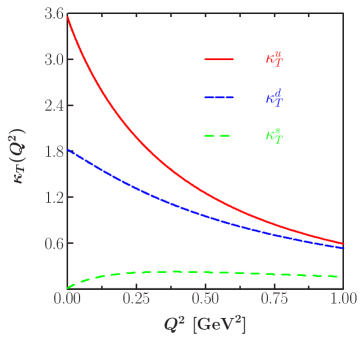
Figure 1: (Color online) The results for the SU(3) flavor-decomposed anomalous tensor magnetic form factors. The solid curve draws the up anomalous tensor magnetic form factor, whereas the dashed and short-dashed ones depict the down and strange ones, respectively. The constituent quark mass $M=420$ MeV is used.

In Fig. 2 we compare the present results of the up and down anomalous tensor magnetic form factors with those of the lattice Hagler:2008 . In order to compare the $Q^{2}$ dependence directly, we have scaled the form factors by the corresponding values at $Q^{2}=0$. This has also the advantage that the renormalization scale dependence is canceled out. In the left panel, we first show the present up form factor and the corresponding lattice one. The lattice result decreases rather slowly as $Q^{2}$ increases, compared to the present result. This is a natural tendency of the lattice calculation because of the large value of the pion mass. We find the similar behavior in the case of the tensor form factor $\delta u(Q^{2})$ Ledwig:2010tu . In the right panel, we draw the result of the down form factor in comparison with that of the lattice calculation. Interestingly, the present result shows almost a similar $Q^{2}$ dependence to the lattice one.

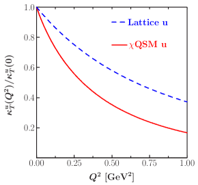
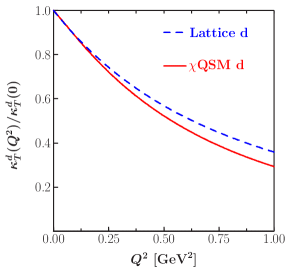
Figure 2: (Color on line) The comparison of the up and down anomalous tensor magnetic form factors with lattice results. The solid curves draw the results of the present work with $M=420$ MeV, whereas the dashed ones depict the lattice results Hagler:2008 . In the left panel, the result of the up anomalous tensor magnetic form factor is compared to that of the lattice. The right panel is for the down form factors. The lattice calculation was performed with $m_{\pi}=600$ MeV.

It is also interesting to parametrize the up and down form factors in a simple form such as

$$\kappa_{T}^{q}(Q^{2})\;=\;\frac{\kappa_{T}^{q}(0)}{\left(1+\frac{Q^{2}}{\alpha M_{\alpha}^{2}}\right)^{\alpha}}\,.$$ (24)

The results for the power $\alpha$ and the pole mass $M_{\alpha}$ are given in Table 6.

Table 6: The parameters for Eq.(24) fitted to the present results of the anomalous tensor magnetic form form factors.

	$\kappa_{T}^{\chi}(0)$	$\alpha$	$M_{\alpha}\,[\mathrm{GeV}]$		$\kappa_{T}^{q}(0)$	$\alpha$	$M_{\alpha}\,[\mathrm{GeV}]$
$\kappa_{T}^{0}(Q^{2})$	$5.39$	$2.82$	$0.74$	$\kappa_{T}^{u}(Q^{2})$	$3.55$	$2.28$	$0.61$
$\kappa_{T}^{3}(Q^{2})$	$1.73$	$5.33$	$0.49$	$\kappa_{T}^{d}(Q^{2})$	$1.82$	$8.12$	$0.86$
$\kappa_{T}^{8}(Q^{2})$	$3.09$	$2.30$	$0.59$

Actually, Göckeler et al. Hagler:2008 have used the ansatz given in Eq.(24) to fit the lattice data. The lattice results of $M_{\alpha}$ for $\kappa_{T}^{u}$ and $\kappa_{T}^{d}$ are given, respectively, as

$$M_{\alpha}^{(u)}\;=\;0.907\,\mathrm{GeV},\;\;\;M_{\alpha}^{(d)}\;=\;0.889\,\mathrm{GeV}.$$ (25)

The power $\alpha=2.5$ was used for all the lattice data. The Fig. 2 can be reproduced with the above given data.

V Summary and outlook

In the present work, we aimed at investigating the anomalous tensor magnetic moments $\kappa_{T}^{q}$ and its corresponding form factors of the proton within the framework of the self-consistent SU(3) and SU(2) chiral quark-soliton model ($\chi$QSM). Generally, the anomalous tensor magnetic moments are given by two contributions: $\kappa_{T}^{q}=-H^{*q}_{T}-\delta q$ where $\delta q$ is the tensor charge and $H^{*q}_{T}$ is a certain linear combination of the form factors appearing in the nucleon matrix element of the tensor current. We first computed the quantities $H^{*q}_{T}$ in the SU(3) and SU(2) version of the $\chi$QSM. We saw that, in contrast to the tensor charges $\delta q$, the quantities $H^{*u,d,s}_{T}$ have in the present framework noticeable contributions from the Dirac-sea and linear strange quark mass corrections. Interestingly, in the case of the SU(3) version these two contributions arrange each other in such a way that their combined SU(3) value is comparable to the SU(2) Dirac-sea value. As a whole, since the valence quark contribution in both versions is nearly the same, we obtain therefore for the components $H^{*u,d}_{T}$ in both versions consistent (comparable) values. For the strange quantity $H^{*s}_{T}$ we see a rather sensitive behavior with respect to the constituent quark mass, the only free parameter in the $\chi$QSM. We regard therefore this quantity to be at the numerical limit of accuracy of the $\chi$QSM. However, we observed for every given numerical setup that the individual parts of $H^{*s}_{T}$ tend to cancel each other. We infer from this that the $\chi$QSM predicts a small $H^{*s}_{T}$.

The tensor charges $\delta q$ were investigated with the present framework in Ref. Ledwig:2010tu . Combining the result of that work with the quanties $H^{*q}_{T}$ of the present one, we were able to predict the anomalous tensor magnetic moments $\kappa_{T}^{u,d,s}$. The values of $\kappa_{T}^{u,d}$ turned out to be positive with the SU(3) values $\kappa_{T}^{u}=3.56$ and $\kappa_{T}^{d}=1.83$ while those of $\kappa_{T}^{s}$ were given in the range of $\kappa_{T}^{s}=0.2\sim-0.2$. This numerical uncertainty for $\kappa_{T}^{s}$ is carried over from $H_{T}^{*s}$ as well as the tendency that the individual parts of $\kappa_{T}^{s}$ are destructively interfereing for any given numerical setup. Accordingly to $H^{*s}_{T}$, we infer that $\kappa_{T}^{s}$ is at the numerical limit of accuracy of the $\chi$QSM but that a small, nearly vanishing $\kappa_{T}^{s}$ is predicted. The SU(2) $\chi$QSM values of $\kappa_{T}^{u,d}$ are: $\kappa_{T}^{u}=3.72$ and $\kappa_{T}^{d}=1.83$ which are comparable to the SU(3) counterparts. We compared the present results of $\kappa_{T}^{u,d}$ with those of other works. They are in qualitative agreement with each other with the hierachy: $4>\kappa_{T}^{u}>\kappa_{T}^{d}>0$ for a renormalization scale below $4\,\textrm{GeV}^{2}$.

We also investigated the anomalous tensor magnetic form factors $\kappa_{T}^{q}(Q^{2})$ of the proton up to a momentum transfer of $Q^{2}=1\,\mathrm{GeV}^{2}$. While the up and down form factors $\kappa_{T}^{u}$ and $\kappa_{T}^{d}$ fall off as $Q^{2}$ increases, the strange form factor $\kappa_{T}^{s}$ starts to grow slowly and then gets lessened mildly from around $0.25$ GeV as $Q^{2}$ increases. This $Q^{2}$ dependence of the strange form factor seems very similar to the neutron electric form factor. We compared the results of the up and down form factors with those of the lattice and found that while for $\kappa_{T}^{u}$ the lattice result falls off more slowly than the present one, the present result for $\kappa_{T}^{d}$ is pretty much similar to the lattice one. By combining the calculation of the electromagnetic form factors with the present results and those of the tensor form factors Ledwig:2010tu , we will be able to get access to the first moment of the transverse quark spin density which yields information on the correlation of transverse coordinate and spin degrees of freedom that are related to the Sivers and Boer-Mulders functions Burkardt:2005 ; Burkardt:2004a . The corresponding investigation is under way.

Appendix A Densities

In this Appendix, we provide the densities for the tensor form factors given Eq. (20), which consist of $\mathcal{Q}_{T0}(r),\cdots,\mathcal{M}_{T2}(r)$. In the following, the sums run freely over all single-quark levels including valence ones except that the sum over $m_{0}$ is constrained to negative-energy levels:

$$\frac{1}{N_{c}}\mathcal{Q}_{T0}(r) = \langle\mathrm{val}|r\rangle i\gamma_{4}\{\frac{z_{1}}{r}\otimes\sigma_{1}\}_{0}\gamma^{5}\langle r|\mathrm{val}\rangle$$ (26)

$$+ \sum_{n}\sqrt{2G_{n}+1}\mathcal{R}_{1}(\varepsilon_{n})\langle n|r\rangle i\gamma_{4}\{\frac{z_{1}}{r}\otimes\sigma_{1}\}_{0}\gamma^{5}\langle r|n\rangle,$$ (27)

$$\frac{1}{N_{c}}\mathcal{X}_{T1}(r) = \sum_{\varepsilon_{n}\neq\varepsilon_{v}}\frac{1}{\varepsilon_{n}-\varepsilon_{v}}(-)^{G_{n}}\langle\mathrm{val}|\tau_{1}|n\rangle\langle n|r\rangle i\gamma_{4}\{\{\frac{z_{1}}{r}\otimes\sigma_{1}\}_{0}\otimes\tau_{1}\}_{1}\gamma^{5}\langle r|\mathrm{val}\rangle$$ (28)

$$+ \frac{1}{2}\sum_{n,m}\mathcal{R}_{5}(\varepsilon_{n},\varepsilon_{m})(-)^{G^{m}-G_{n}}\langle n|\tau_{1}|m\rangle\langle m|r\rangle i\gamma_{4}\{\{\frac{z_{1}}{r}\otimes\sigma_{1}\}_{0}\otimes\tau_{1}\}_{1}\gamma^{5}\langle r|n\rangle,$$ (29)

$$\frac{1}{N_{c}}\mathcal{X}_{T2}(r) = \sum_{n^{0}}\frac{1}{\varepsilon_{n^{0}}-\varepsilon_{v}}\sqrt{2G_{n}+1}\left[\langle\mathrm{val}|n^{0}\rangle\langle\mathrm{val}|r\rangle i\gamma_{4}\{\frac{z_{1}}{r}\otimes\sigma_{1}\}_{0}\gamma^{5}\langle r|n^{0}\rangle\right]$$ (30)

$$+ \sum_{n,m^{0}}\mathcal{R}_{5}(\varepsilon_{n},\varepsilon_{m^{0}})\sqrt{2G_{n}+1}\left[\langle n|m^{0}\rangle\langle n|r\rangle i\gamma_{4}\{\frac{z_{1}}{r}\otimes\sigma_{1}\}_{0}\gamma^{5}\langle r|m^{0}\rangle\right],$$ (31)

$$\frac{1}{N_{c}}\mathcal{M}_{T0}(r) = \sum_{\varepsilon_{n}\neq\varepsilon_{v}}\frac{1}{\varepsilon_{n}-\varepsilon_{v}}\langle\mathrm{val}|r\rangle i\gamma_{4}\{\frac{z_{1}}{r}\otimes\sigma_{1}\}_{0}\gamma^{5}\langle r|n\rangle\langle n|\gamma_{4}|\mathrm{val}\rangle$$ (32)

$$- \frac{1}{2}\sum_{n,m}\sqrt{2G_{n}+1}\langle n|\gamma_{4}|m\rangle\langle m|r\rangle i\gamma_{4}\{\frac{z_{1}}{r}\otimes\sigma_{1}\}_{0}\gamma^{5}\langle r|n\rangle\mathcal{R}_{2}(\varepsilon_{n},\varepsilon_{m}),$$ (33)

$$\frac{1}{N_{c}}\mathcal{M}_{T1}(r) = \sum_{\varepsilon_{n}\neq\varepsilon_{v}}\frac{(-)^{G_{n}}}{\varepsilon_{n}-\varepsilon_{v}}\langle\mathrm{val}|r\rangle i\gamma_{4}\{\{\frac{z_{1}}{r}\otimes\sigma_{1}\}_{0}\otimes\tau_{1}\}_{1}\gamma^{5}\langle r|n\rangle\langle n|\gamma_{4}\tau_{1}|\mathrm{val}\rangle$$ (34)

$$- \frac{1}{2}\sum_{n,m}(-)^{G_{m}-G_{n}}\langle n|\gamma_{4}\tau_{1}|m\rangle\langle m|r\rangle i\gamma_{4}\{\{\frac{z_{1}}{r}\otimes\sigma_{1}\}_{0}\otimes\tau_{1}\}_{1}\gamma^{5}\langle r|n\rangle\mathcal{R}_{2}(\varepsilon_{n},\varepsilon_{m}),$$ (35)

$$\frac{1}{N_{c}}\mathcal{M}_{T2}(r) = \sum_{n^{0}}\frac{1}{\varepsilon_{n^{0}}-\varepsilon_{v}}\langle\mathrm{val}|r\rangle i\gamma_{4}\{\frac{z_{1}}{r}\otimes\sigma_{1}\}_{0}\gamma^{5}\langle r|n^{0}\rangle\langle n^{0}|\gamma_{4}|\mathrm{val}\rangle$$ (36)

$$- \sum_{n,m^{0}}\sqrt{2G_{n}+1}\langle m^{0}|r\rangle i\gamma_{4}\{\frac{z_{1}}{r}\otimes\sigma_{1}\}_{0}\gamma^{5}\langle r|n\rangle\langle n|\gamma_{4}|m^{0}\rangle\mathcal{R}_{2}(\varepsilon_{n},\varepsilon_{m^{0}}),$$ (37)

where the regularization functions are given by:

$$\mathcal{R}_{1}(\varepsilon_{n}) = -\frac{1}{2\sqrt{\pi}}\varepsilon_{n}\int_{1/\Lambda^{2}}^{\infty}\frac{du}{\sqrt{u}}e^{-u\varepsilon_{n}^{2}}\,\,,$$ (38)

$$\mathcal{R}_{2}(\varepsilon_{n},\varepsilon_{m}) = \int_{1/\Lambda^{2}}^{\infty}du\frac{1}{2\sqrt{\pi u}}\frac{\varepsilon_{m}e^{-u\varepsilon_{m}^{2}}-\varepsilon_{n}e^{-u\varepsilon_{n}^{2}}}{\varepsilon_{n}-\varepsilon_{m}}\,\,,$$ (39)

$$\mathcal{R}_{5}(\varepsilon_{n},\varepsilon_{m}) = \frac{1}{2}\frac{\textrm{sign}\varepsilon_{n}-\textrm{sign}\varepsilon_{m}}{\varepsilon_{n}-\varepsilon_{m}}\,\,.$$ (40)

References

• (1) J. P. Ralston and D. E. Soper, Nucl. Phys.  B 172 (1980) 445.
• (2) R. L. Jaffe and X. D. Ji, Nucl. Phys.  B 375 (1992) 527.
• (3) J. L. Cortes, B. Pire and J. P. Ralston, Z. Phys.  C 55 (1992) 409.
• (4) V. Barone, A. Drago, P. G. Ratcliffe, Phys. Rept. 359 (2002) 1.
• (5) S. Boffi, B. Pasquini, Riv. Nuovo Cim. 30 (2007) 387.
• (6) A.V. Efremov, K. Goeke, P. Schweitzer, Eur. Phys. J. C 35 (2004) 207.
• (7) V. Barone, [PAX Collaboration], hep-ex/0505054.
• (8) M. Anselmino, V. Barone, A. Drago, N.N. Nikolaev, Phys. Lett. B 594 (2004) 97.
• (9) B. Pasquini, M. Pincetti, S. Boffi, Phys. Rev. D 76 (2007) 034020.
• (10) M. Anselmino, M. Boglione, U. D’Alesio, A. Kotzinian, F. Murgia, A. Prokudin, C. Turk, Phys. Rev. D 75 (2007) 054032.
• (11) M. Diehl, Eur. Phys. J. C 19 (2001) 485.
• (12) P. Hägler, Phys. Lett. B 594 (2004) 164.
• (13) T. Ledwig, A. Silva and H.-Ch. Kim, arXiv:1004.3612 [hep-ph].
• (14) H.-X. He, X.-D. Ji, Phys. Rev. D 52 (1995) 2960.
• (15) M. Diehl, Ph. Hägler, Eur. Phys. J. C 44 (2005) 87.
• (16) M. Burkardt, Phys. Rev. D 72 (2005) 094020.
• (17) D. Boer, P.J. Mulders, Phys. Rev. D 57 (1998) 5780.
• (18) D. W. Sivers, Phys. Rev. D 43 (1991) 261.
• (19) M. Burkardt, Nucl. Phys. A 735 (2004) 185.
• (20) M. Burkardt and D. S. Hwang, Phys. Rev. D 69 (2004) 074032.
• (21) M. Burkardt, Phys. Rev. D 69 (2004) 057501.
• (22) HERMES Collaboration (A. Airapetian et al.), Phys. Rev. Lett. 94 (2005) 012002.
• (23) M. Burkardt, Phys. Lett. B 639 (2006) 462.
• (24) K. Abe et al. [Belle Colaboration], Phys. Rev. Lett. 96 (2006) 232002.
• (25) L. Pappalardo for the HERMES collaboration, Apr 2006. 4pp. Prepared for 14th International Workshop on Deep Inelastic Scattering (DIS 2006), Tsukuba, Japan, 20-24 Apr 2006.
• (26) E.S. Ageev et al., [COMPASS Collaboration], Nucl. Phys. B 765 (2007) 31.
• (27) M. Anselmino, M. Boglione, U. D’Alesio, A. Kotzinian, F. Murgia, A. Prokudin, S. Melis, Nucl. Phys. Proc. Suppl. 191 (2009) 98.
• (28) B. Pasquini, M. Pincetti, S. Boffi, Phys. Rev. D 72 (2005) 094029.
• (29) B. Pasquini, S. Boffi, Phys. Lett. B 653 (2007) 23.
• (30) M. Göckeler et al. [QCDSF Collaboration and UKQCD Collaboration], Phys. Rev. Lett. 98 (2007) 222001.
• (31) M. Wakamatsu, Phys. Rev. D 79 (2009) 014033.
• (32) M. Burkardt, B. Hannafious, Phys. Lett. B 658 (2008) 130.
• (33) C.V. Christov et al., Prog. Part. Nucl. Phys. 37 (1996) 91.
• (34) D. Diakonov, V. Y. Petrov and P. V. Pobylitsa, Nucl. Phys.  B 306, 809 (1988).
• (35) D. Diakonov, Lectures given at Advanced Summer School on Nonperturbative Quantum Field Physics, Peniscola, Spain, 2-6 Jun 1997, hep-ph/9802298.
• (36) D. Diakonov and V. Y. Petrov, Nucl. Phys.  B 245, 259 (1984).
• (37) D. Diakonov and V. Y. Petrov, Nucl. Phys.  B 272, 457 (1986).
• (38) M. Gluck, E. Reya, A. Vogt, Z. Phys. C 67 (1995) 433.
• (39) A. Silva, H.-Ch. Kim, K. Goeke, Phys. Rev. D 65 (2002) 014016, Erratum-ibid. 66 (2002) 039902.
• (40) H.-Ch. Kim, A. Blotz, M.V. Polyakov and K. Goeke, Phys. Rev. D 53 (1996) 4013.
• (41) A. Blotz, D. Diakonov, K. Goeke, N. W. Park, V. Petrov and P. V. Pobylitsa, Nucl. Phys.  A 555 (1993) 765.
• (42) M. Praszalowicz, T. Watabe, K. Goeke, Nucl. Phys. A 647 (1999) 49.