Exact Solution for Optimal Navigation with Total Cost Restriction

Abstract

Recently, Li et al. have concentrated on Kleinberg’s navigation model with a certain total length constraint $\Lambda=cN$, where $N$ is the number of total nodes and $c$ is a constant. Their simulation results for the 1- and 2-dimensional cases indicate that the optimal choice for adding extra long-range connections between any two sites seems to be $\alpha=d+1$, where $d$ is the dimension of the lattice and $\alpha$ is the power-law exponent. In this paper, we prove analytically that for the 1-dimensional large networks, the optimal power-law exponent is $\alpha=2$ Further, we study the impact of the network size and provide exact solutions for time cost as a function of the power-law exponent $\alpha$. We also show that our analytical results are in excellent agreement with simulations.

1 Introduction

Since Milgram and his cooperators conducted the first small-world experiment in the 1960s, much attention has been dedicated to the problem of navigation in real social networks. The first navigation model was proposed by Kleinberg[1]. He employed an $L\times L$ square lattice, where in addition to the links between nearest neighbors each node $i$ was connected to a random node $j$ with a probability $P_{ij}\propto r_{ij}^{-\alpha}$ ($r_{ij}$ denotes the lattice distance between nodes $i$ and $j$). Kleinberg has proved that when $\alpha=d$, where $d$ is the dimension of the lattice, the optimal time cost of navigation with a decentralized algorithm is at most $O(\log^{2}L)$. The optimal case indicates that individuals are able to find short paths effectively with only local information, which can explain six degrees of separation quite well. In recent years, further studies on Kleinberg’s navigation model have been developed [2, 4, 6, 3, 7, 5, 8]. Roberson et al. study the navigation problem in fractal small-world networks [2], where they prove that $\alpha=d$ is also the optimal power-law exponent in the fractal case. Cartozo et al. use dynamical equations to study the process of Kleinberg navigation [4, 3]. They provide an exact solution for the asymptotic behavior of such a greedy algorithm as a function of the dimension $d$ of the lattice and the power-law exponent $\alpha$. Yang et al. construct a network with limited cost $\Lambda=C$. The limited cost $\Lambda$ represents the total length of the long-range connections which are added with power-law distance distribution $P(r)=a{r^{-\alpha}}$ [5] in one-dimensional space. They find that the network has the smallest average shortest path when $\alpha=2$. More recently, Li et al. have considered Kleinberg’s navigation model with a total cost constraint [6]. In their model, the total length of the long-range connections is restricted to $\Lambda=c\cdot N$, where $N$ represents the total number of nodes in the lattice based network and $c$ is a positive constant. Their results show that the best transport condition(minimal number of steps to reach the target) is obtained with a power-law exponent $\alpha=d+1$ for constrained navigation in a $d$-dimensional lattice in the 1 and 2-dimensional cases. In this paper, we give a rigorous theoretical analysis of the optimal condition $\alpha=2$ for navigation and provide the exact time cost for various power-law exponents $\alpha$ on the 1-dimensional cost constrained network.

2 Dynamical Equations for One-Dimensional Navigation with Cost Restriction

We consider the one-dimensional navigation problem on a cycle with $N=4n$ nodes. For the sake of simplicity, we assume that each node has only two short-range connections to its two nearest neighbors, and the probability of having a long-range connection satisfies to a certain power-law distribution. Obviously, the largest possible length of a long-range connection is $2n$ in this cycle. We number all nodes inclusively from $0$ to $4n-1$ and assume that the navigation process starts from the node $0$ and ends at the node $n$ for further simplification. The network is illustrated in FIG.1.

According to the discussion above, the probability of a long-range connection between any given pair of nodes with a distance $r$ is

$$p(r,\alpha)=\frac{{r^{-\alpha}}}{2{\sum\limits_{r=1}^{2n}{r^{-\alpha}}}},\alpha\geq 0,$$ (1)

where $\alpha$ is the power exponent of the power-law distribution. The expected length of the long-range connection from any node satisfies $E(L_{\alpha})=2\sum\limits_{r=1}^{2n}{r\cdot p(r,\alpha)}$. To be consistent with Li’s work[6], in this paper we set the total cost limit to $\Lambda=c\cdot 4n$, where $c$ is a positive constant and $4n$ is the number of nodes on the cycle. Subject to this limit, the expected number of long-range connections on the whole cycle can be written as $E(N_{\alpha}){\rm{=}}\frac{\Lambda}{{E(L_{\alpha})}}$.

Since all nodes are homogeneous, we know that the number of directed long-range connections from each node should obey the Poisson distribution with a parameter $\lambda=\frac{{E(N_{\alpha})}}{4n}$. Thus, the probability of a one long-range connection from each node can be given by $\lambda e^{-\lambda}$. When $\lambda$ is small enough, the probability of the existence two or more than two long-range connections for a arbitrary node can be ignored. More over, for a given node and distance $r$, there are only two nodes which satisfy the condition that the distances between them and the given node be $r$. So, if $\lambda$ is too large, we cannot construct a spatial network on which the length of long-rang connections is power law distribution. According to the above two reasons, in this paper we only consider the case where navigation process is carried out by at most one long-range connection ($c$ is small) for each node.

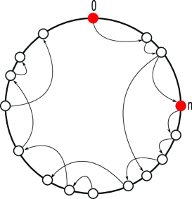
Figure 1: The navigation model in this paper. Node $0$ is the starting node, and node $n$ is the target.

If we use $E(L_{s}^{\alpha})$ to denote the expected distance by a long-range connection from a node $s$ toward the target node $n$, then we have

$$E(L_{s}^{\alpha})=\sum\limits_{r=1}^{n-s}{r\cdot p(r,\alpha)}+\sum\limits_{r=n-s+1}^{2n-2s-1}{(2n-2s-r)\cdot p(r,\alpha)}.$$ (2)

We further denote the expected distance by an edge (long or short range) from a node $s$ toward the target node $n$ as $E(J_{s})$. Then we have

$$E(J_{s})=\lambda e^{-\lambda}\cdot E(L_{s}^{\alpha})+1-\lambda e^{-\lambda}\cdot[\sum\limits_{r=1}^{n-s}{p(r,\alpha)}+\sum\limits_{r=n-s+1}^{2n-2s-1}{p(r,\alpha)}]$$ (3)

For simplicity, we consider the continuous form of all equations provided above. Then $\lambda$ can be written as

$$\lambda=\begin{cases}c\frac{2}{{2n+1}},&\alpha=0\\ c\frac{{\ln 2n}}{{2n}},&\alpha=1\\ c\frac{{1-\frac{1}{{2n}}}}{{\ln 2n}},&\alpha=2\\ c\frac{{\alpha-2}}{{\alpha-1}}\cdot\frac{{{{(2n)}^{1-\alpha}}-1}}{{{{(2n)}^{2-\alpha}}-1}},&else.\\ \end{cases}$$ (4)

When the network size is large enough, Eq.(4) can be simplified to

$$\lambda=\begin{cases}0,&0\leq\alpha\leq 2\\ c\frac{{\alpha-2}}{{\alpha-1}},&else.\\ \end{cases}$$ (5)

The method of dynamical equations is used to deduce the searching time with limited total cost. Suppose that at time $t$, the corresponding position is $s(t)$. Obviously, $s(0)=0$ holds. The dynamical equation can be written as

$$\left\{\begin{array}[]{l}\frac{{ds}}{{dt}}=E(J_{s}),\\ s(0)=0.\\ \end{array}\right.$$ (6)

Before solving Eq.(6), we first study the optimal power-law exponent $\alpha$ by comparing $E(J_{s})$ (Eq.(3)) under different values of $\alpha$. We rewrite the distance to the target $n-s$ as $\varepsilon n$, where $0<\varepsilon\leq 1$ is a constant. For any given $0<\varepsilon\leq 1$, we assume $\varepsilon n$ is large enough, such that long-range connections will be used in the search process. Finally, Eq.(3) can be simplified to the following forms,

$$E(J_{s})\sim\begin{cases}\frac{1}{4}\varepsilon^{2}c+1,&\alpha=0\\ \frac{{\ln 2}}{2}\varepsilon c+1,&\alpha=1\\ \frac{1}{2}c+1,&\alpha=2\\ \frac{e^{-c\frac{{\alpha-2}}{{\alpha-1}}}}{{2(\alpha-1)}}c+1,&\alpha>2\\ \frac{{2^{\alpha-1}-1}}{{2(\alpha-1)}}\varepsilon^{2-\alpha}c+1,&else\\ \end{cases}$$ (7)

It is not difficult to show the right side of the Eq.(7) monotonically increases with $\alpha$ for $0\leq\alpha\leq 2$ and decreases with $\alpha$ for $\alpha>2$. We can also prove that $E(J_{s})$ is continuous at the point $\alpha=2$. Overall, $E(J_{s})$ is continuous and reaches its maximal value at $\alpha=2$ for any given $\varepsilon$. It has been revealed that the optimal condition for navigation with limited cost is a tradeoff between the length and the number of long-range connections added to the cycle. Prior to solving the dynamical equations theoretically, we have already shown that the optimal power-law exponent is $\alpha=2$ with some proper simplifications.

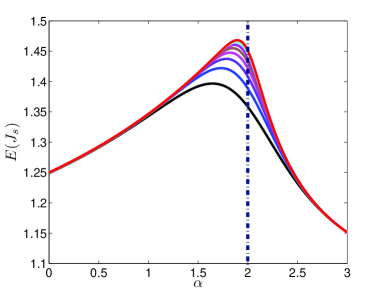
Figure 2: Effects of the network size $n$ on the numerical results. The network size is $10^{\beta}$, and $\beta$ is chosen from 3 to 10 from bottom to top. It can be seen that the optimal choice of $\alpha$ gets closer to $\alpha=2$ as $n$ increases.

3 Results

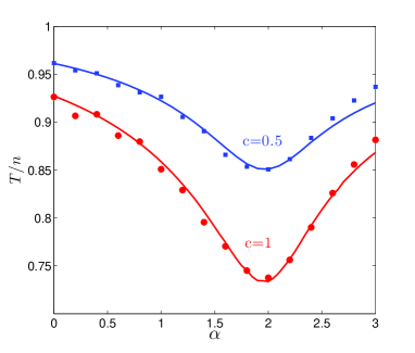
Figure 3: Comparison between numerical results and simulation results for $c=0.5$ and $c=1$ respectively. The curves represent the numerical results while the squares denote the simulation results with $n=10000$. It is shown that our numerical solutions are consistent with the simulation results and both of them have the optimal value at $\alpha=2$ approximately.

As discussed above, the optimal power-law exponent for navigation in a 1-dimensional large network is $\alpha=2$. FIG.2 represents the size effect on $E(J_{s})$. It can be found that $\alpha=2$ is the optimal power-law exponent when the network size goes to infinity.

To obtain exact time cost of navigation with cost restriction, Eq.(6) should be solved. In the following, we will first give its numerical results and then derive its exact solutions for various values of $\alpha$. The Ronge-Kutta method has been introduced to solve the dynamical equation numerically and the results are presented in FIG.3. It shows that the optimal power-law exponent is $\alpha=2$. To check up our method, we also perform search experiments on the one-dimensional cycle. The comparison between our analytical results and the simulation results with $c=0.5$ and $c=1$ are given by FIG.3. As can be seen, they agree quite well and both of them obtain the optimal navigation at $\alpha=2$.

It is able to get the exact solutions of navigation with limited cost for various values of $\alpha$. For instance, the dynamical equation in the case $\alpha=0$ is,

$$\frac{{ds}}{{dt}}=\frac{{c(n-s-1)^{2}}}{{4n^{2}}}+1.$$ (8)

Based on the initial condition $s(0)=0$, we can get the exact solution of Eq.(8).

Here, we use $T$ to denote the time cost for getting the destination node $n$. We should have $T=\frac{2n}{{\sqrt{c}}}\arctan\frac{{\sqrt{c}}}{2}$ for large enough $n$. Thus, the average required time to navigate from the source node to the target satisfies

$$\frac{T}{n}=\frac{2}{{\sqrt{c}}}\arctan\frac{{\sqrt{c}}}{2}.$$ (9)

Analogously, the exact solution for exponent $\alpha$ when $n$ approaches infinity are acquired as

$$\frac{T}{n}=\begin{cases}\frac{2}{{\sqrt{c}}}\arctan\frac{{\sqrt{c}}}{2},&\alpha=0\\ \frac{2}{{c\ln 2}}\ln\frac{{c\ln 2+2}}{2},&\alpha=1\\ \frac{{2(\alpha-1)}}{{2(\alpha-1)+ce^{-c\frac{{\alpha-2}}{{\alpha-1}}}}},&\alpha\geq 2.\\ \end{cases}$$ (10)

The above results suggest that the relationship between the exact time cost and the distance is linear for most values of $\alpha$. Meanwhile, we have studied the size effect on navigation with cost constraint. Based on Eq.(4), we know that $\lambda$ approaches its limit much more slower when $\alpha$ gets closer to 2 as $n$ increases. The time cost of navigation with different network sizes are provided in FIG.4. It can be verified that it will approach its limit as $n$ goes to infinity, which is given by Eq.(10).

In summary, we constructed a the dynamical equation for the 1-dimensional navigation with limited cost. Based on the equation, we proved that for large networks and comparatively small cost the optimal power-law exponent is $\alpha=2$. Our analytical results confirm the previous simulations[6] well.

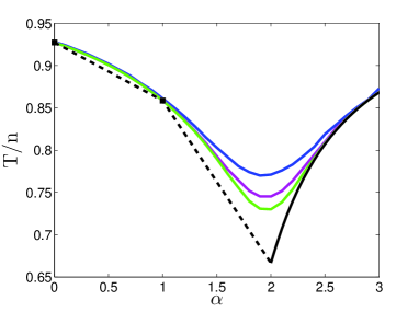
Figure 4: Size effect on navigation. The exact solutions are obtained on the 1-dimensional cycle with parameter $c=1$. The network size $n$ is $10^{\beta}$, and parameter $\beta$ values of the upper three solid curves are chosen from 3 to 5 from top to bottom. It is shown that $\alpha=2$ is always the optimal choice for various values of $n$. The bottom line, obtained when $n$ goes infinity, represents the exact solutions of the navigation process with limited cost. Notice that we only provide the exact solutions at $\alpha=0$ and $\alpha=1$ when $\alpha<2$, thus we only connect the two exact points with dashed lines.

Acknowledgement.We wish to thank Prof. Shlomo Havlin for some useful discussions and two anonymous referees for their helpful suggestions. This work is partially supported by the Fundamental Research Funds for the Central Universities and NSFC under Grant No. 70771011 and 60974084. Y. Hu is supported by Scientific Research Foundation and Excellent Ph.D Project of Beijing Normal University.

References

- [1] \Name Kleinberg J. \REVIEWNature4062000845.
- [2] \Name Roberson M. R. Ben-Avraham D. \REVIEWPhys. Rev. E74200617101.
- [3] \NameCaretta Cartozo C. De Los Rios P. \REVIEWPhys. Rev. Lett.1022009238703.
- [4] \NameCarmi S., Carter S., Sun J. Ben-Avraham D. \REVIEWPhys. Rev. Lett.1022009238702.
- [5] \NameYang H., Nie Y., Zeng A., Fan Y., Hu Y. Di Z. \REVIEWEPL89201058002.
- [6] \NameLi G., Reis S. D. S., Moreira A. A., Havlin S., Stanley H. E. Andrade, Jr. J. S. \REVIEWPhys. Rev. Lett.1042010018701.
- [7] \NameBarri re L.,Fraigniaud P., Kranakis E., Krizanc D. \REVIEWSpringer,New York2001.
- [8] \NameHu Y., Wang Y., Li D., Havlin S., Di Z. \REVIEWarXiv:1002.18022010.