Shifted Power Method for Computing Tensor Eigenpairsthanks: This work was funded by the applied mathematics program at the U.S. Department of Energy and by an Excellence Award from the Laboratory Directed Research & Development (LDRD) program at Sandia National Laboratories. Sandia National Laboratories is a multiprogram laboratory operated by Sandia Corporation, a wholly owned subsidiary of Lockheed Martin Corporation, for the United States Department of Energy’s National Nuclear Security Administration under contract DE-AC04-94AL85000.

Tamara G. Kolda222Sandia National Laboratories, Livermore, CA. Email: {tgkolda,jmayo}@sandia.gov.    Jackson R. Mayo222Sandia National Laboratories, Livermore, CA. Email: {tgkolda,jmayo}@sandia.gov.
Abstract

Recent work on eigenvalues and eigenvectors for tensors of order m3𝑚3m\geq 3 has been motivated by applications in blind source separation, magnetic resonance imaging, molecular conformation, and more. In this paper, we consider methods for computing real symmetric-tensor eigenpairs of the form 𝓐𝐱m1=λ𝐱𝓐superscript𝐱𝑚1𝜆𝐱\bm{\mathscr{{A}}}{\bm{\mathbf{{x}}}}^{m-1}=\lambda{\bm{\mathbf{{x}}}} subject to 𝐱=1norm𝐱1\|{\bm{\mathbf{{x}}}}\|=1, which is closely related to optimal rank-1 approximation of a symmetric tensor. Our contribution is a shifted symmetric higher-order power method (SS-HOPM), which we show is guaranteed to converge to a tensor eigenpair. SS-HOPM can be viewed as a generalization of the power iteration method for matrices or of the symmetric higher-order power method. Additionally, using fixed point analysis, we can characterize exactly which eigenpairs can and cannot be found by the method. Numerical examples are presented, including examples from an extension of the method to finding complex eigenpairs.

keywords:
tensor eigenvalues, E-eigenpairs, Z-eigenpairs, l2superscript𝑙2l^{2}-eigenpairs, rank-1 approximation, symmetric higher-order power method (S-HOPM), shifted symmetric higher-order power method (SS-HOPM)
AMS:
15A18, 15A69
\opt

draft

\opt

siam

\opt

draft \optarXiv,siam

1 Introduction

Tensor eigenvalues and eigenvectors have received much attention lately in the literature [13, 18, 20, 19, 4, 15, 27]. The tensor eigenproblem is important because it has applications in blind source separation [11], magnetic resonance imaging [25, 22], molecular conformation [7], etc. There is more than one possible definition for a tensor eigenpair [18]; in this paper, we specifically use the following definition.

Definition 1.

Assume that 𝓐𝓐\bm{\mathscr{{A}}} is a symmetric mthsuperscript𝑚thm^{\text{th}}-order n𝑛n-dimensional real-valued tensor. For any n𝑛n-dimensional vector 𝐱𝐱{\bm{\mathbf{{x}}}}, define

(𝓐𝐱m1)i1i2=1nim=1nai1i2imxi2ximfori1=1,,n.formulae-sequencesubscript𝓐superscript𝐱𝑚1subscript𝑖1superscriptsubscriptsubscript𝑖21𝑛superscriptsubscriptsubscript𝑖𝑚1𝑛subscript𝑎subscript𝑖1subscript𝑖2subscript𝑖𝑚subscript𝑥subscript𝑖2subscript𝑥subscript𝑖𝑚forsubscript𝑖11𝑛\left(\bm{\mathscr{{A}}}{\bm{\mathbf{{x}}}}^{m-1}\right)_{i_{1}}\equiv\sum_{i_{2}=1}^{n}\cdots\sum_{i_{m}=1}^{n}{a}_{i_{1}i_{2}\cdots i_{m}}{x}_{i_{2}}\cdots{x}_{i_{m}}\quad\text{for}\quad i_{1}=1,\dots,n. (1)

Then λ𝜆\lambda\in\mathbb{R} is an eigenvalue of 𝓐𝓐\bm{\mathscr{{A}}} if there exists 𝐱n𝐱superscript𝑛{\bm{\mathbf{{x}}}}\in\mathbb{R}^{n} such that

𝓐𝐱m1=λ𝐱and𝐱T𝐱=1.formulae-sequence𝓐superscript𝐱𝑚1𝜆𝐱andsuperscript𝐱𝑇𝐱1\bm{\mathscr{{A}}}{\bm{\mathbf{{x}}}}^{m-1}=\lambda{\bm{\mathbf{{x}}}}\quad\text{and}\quad{\bm{\mathbf{{x}}}}^{T}{\bm{\mathbf{{x}}}}=1. (2)

The vector 𝐱𝐱{\bm{\mathbf{{x}}}} is a corresponding eigenvector, and (λ,𝐱)𝜆𝐱(\lambda,{\bm{\mathbf{{x}}}}) is called an eigenpair.

Definition 1 is equivalent to the Z-eigenpairs defined by Qi [18, 19] and the l2superscript𝑙2l^{2}-eigenpairs defined by Lim [13]. In particular, Lim [13] observes that any eigenpair (λ,𝐱)𝜆𝐱(\lambda,{\bm{\mathbf{{x}}}}) is a Karush-Kuhn-Tucker (KKT) point (i.e., a constrained stationary point) of the nonlinear optimization problem

max𝐱n𝓐𝐱msubject to𝐱T𝐱=1,where𝓐𝐱mi1=1nim=1nai1imxi1xim.formulae-sequencesubscript𝐱superscript𝑛𝓐superscript𝐱𝑚subject tosuperscript𝐱𝑇𝐱1where𝓐superscript𝐱𝑚superscriptsubscriptsubscript𝑖11𝑛superscriptsubscriptsubscript𝑖𝑚1𝑛subscript𝑎subscript𝑖1subscript𝑖𝑚subscript𝑥subscript𝑖1subscript𝑥subscript𝑖𝑚\max_{{\bm{\mathbf{{x}}}}\in\mathbb{R}^{n}}\bm{\mathscr{{A}}}{\bm{\mathbf{{x}}}}^{m}\quad\text{subject to}\quad{\bm{\mathbf{{x}}}}^{T}{\bm{\mathbf{{x}}}}=1,\quad\text{where}\quad\bm{\mathscr{{A}}}{\bm{\mathbf{{x}}}}^{m}\equiv\sum_{i_{1}=1}^{n}\cdots\sum_{i_{m}=1}^{n}{a}_{i_{1}\cdots i_{m}}{x}_{i_{1}}\cdots{x}_{i_{m}}. (3)

This is equivalent to the problem of finding the best symmetric rank-1 approximation of a symmetric tensor [6]. We present the more general definition that incorporates complex-valued eigenpairs in §5.

In this paper, we build upon foundational work by Kofidis and Regalia [11] for solving (3). Their paper is extremely important for computing tensor eigenvalues even though it predates the definition of the eigenvalue problem by three years. Kofidis and Regalia consider the higher-order power method (HOPM) [6], a well-known technique for approximation of higher-order tensors, and show that its symmetric generalization (S-HOPM) is not guaranteed to converge. They go on, however, to use convexity theory to provide theoretical results (as well as practical examples) explaining conditions under which the method is convergent for even-order tensors (i.e., m𝑚m even). Further, these conditions are shown to hold for many problems of practical interest.

In the context of independent component analysis (ICA), both Regalia and Kofidis [23] and Erdogen [8] have developed shifted variants of the power method and shown that they are monotonically convergent. We present a similar method in the context of finding real-valued tensor eigenpairs, called the shifted symmetric higher-order power method (SS-HOPM), along with theory showing that it is guaranteed to converge to a constrained stationary point of (3). The proof is general and works for both odd- and even-order tensors (i.e., all m3𝑚3m\geq 3). The effectiveness of SS-HOPM is demonstrated on several examples, including a problem noted previously [11] for which S-HOPM does not converge. We also present a version of SS-HOPM for finding complex-valued tensor eigenpairs and provide examples of its effectiveness.

As mentioned, there is more than one definition of a tensor eigenpair. In the case of the lmsuperscript𝑙𝑚l^{m}-eigenpair (we use m𝑚m for the tensor order instead of k𝑘k as in some references) or H-eigenpair, the eigenvalue equation becomes 𝓐𝐱m1=λ𝐱[m1]𝓐superscript𝐱𝑚1𝜆superscript𝐱delimited-[]𝑚1\bm{\mathscr{{A}}}{\bm{\mathbf{{x}}}}^{m-1}=\lambda{\bm{\mathbf{{x}}}}^{[m-1]}, where 𝐱[m1]superscript𝐱delimited-[]𝑚1{\bm{\mathbf{{x}}}}^{[m-1]} denotes the vector 𝐱𝐱{\bm{\mathbf{{x}}}} with each element raised to the (m1)stsuperscript𝑚1st(m-1)^{\text{st}} power [13, 18]. In this context, Qi, Wang, and Wang [21] propose some methods specific to third-order tensors (m=3𝑚3m=3). Unlike the (l2superscript𝑙2l^{2}-)eigenvalues we consider here, it is possible to guarantee convergence to the largest lmsuperscript𝑙𝑚l^{m}-eigenvalue for certain classes of nonnegative tensors. For example, see the power methods proposed by Ng, Qi, and Zhou [15] and Liu, Zhou, and Ibrahim [14], the latter of which also uses a shift to guarantee convergence for any irreducible nonnegative tensor.

2 Preliminaries

Throughout, let ΓΓ\Gamma and ΣΣ\Sigma denote the unit ball and sphere on nsuperscript𝑛\mathbb{R}^{n}, i.e.,

Γ={𝐱n:𝐱1}andΣ={𝐱n:𝐱=1}.formulae-sequenceΓconditional-set𝐱superscript𝑛norm𝐱1andΣconditional-set𝐱superscript𝑛norm𝐱1\Gamma=\{{\bm{\mathbf{{x}}}}\in\mathbb{R}^{n}:\|{\bm{\mathbf{{x}}}}\|\leq 1\}\quad\text{and}\quad\Sigma=\{{\bm{\mathbf{{x}}}}\in\mathbb{R}^{n}:\|{\bm{\mathbf{{x}}}}\|=1\}.

Additionally, define

Πmthe set of all permutations of (1,,m).subscriptΠ𝑚the set of all permutations of 1𝑚\Pi_{m}\equiv\text{the set of all permutations of }(1,\dots,m).

Let 𝐱𝐲bottom𝐱𝐲{\bm{\mathbf{{x}}}}\bot{\bm{\mathbf{{y}}}} denote 𝐱T𝐲=0superscript𝐱𝑇𝐲0{\bm{\mathbf{{x}}}}^{T}{\bm{\mathbf{{y}}}}=0, and define 𝐱{𝐲n:𝐱𝐲}superscript𝐱bottomconditional-set𝐲superscript𝑛bottom𝐱𝐲{\bm{\mathbf{{x}}}}^{\bot}\equiv\{{\bm{\mathbf{{y}}}}\in\mathbb{R}^{n}:{\bm{\mathbf{{x}}}}\bot{\bm{\mathbf{{y}}}}\}. Let ρ(𝐀)𝜌𝐀\rho({\bm{\mathbf{{A}}}}) denote the spectral radius of a square matrix 𝐀𝐀{\bm{\mathbf{{A}}}}, i.e., the maximum of the magnitudes of its eigenvalues.

2.1 Tensors

A tensor is an m𝑚m-way array. We let [m,n]superscript𝑚𝑛\mathbb{R}^{[m,n]} denote the space of mthsuperscript𝑚thm^{\text{th}}-order real-valued tensors with dimension n𝑛n, e.g., [3,2]=2×2×2superscript32superscript222\mathbb{R}^{[3,2]}=\mathbb{R}^{2\times 2\times 2}. We adopt the convention that [0,n]=superscript0𝑛\mathbb{R}^{[0,n]}=\mathbb{R}.

We formally introduce the notion of a symmetric tensor, sometimes also called supersymmetric, which is invariant under any permutation of its indices. Further, we define a generalization of the tensor-vector multiplication in equations (1) and (3).

Definition 2 (Symmetric tensor [5]).

A tensor 𝓐[m,n]𝓐superscript𝑚𝑛\bm{\mathscr{{A}}}\in\mathbb{R}^{[m,n]} is symmetric if

aip(1)ip(m)=ai1imfor alli1,,im{1,,n}andpΠm.formulae-sequencesubscript𝑎subscript𝑖𝑝1subscript𝑖𝑝𝑚subscript𝑎subscript𝑖1subscript𝑖𝑚for allsubscript𝑖1formulae-sequencesubscript𝑖𝑚1𝑛and𝑝subscriptΠ𝑚{a}_{i_{p(1)}\cdots i_{p(m)}}={a}_{i_{1}\cdots i_{m}}\quad\text{for all}\quad i_{1},\dots,i_{m}\in\{1,\dots,n\}\quad\text{and}\quad p\in\Pi_{m}.
Definition 3 (Symmetric tensor-vector multiply).

Let 𝓐[m,n]𝓐superscript𝑚𝑛\bm{\mathscr{{A}}}\in\mathbb{R}^{[m,n]} be symmetric and 𝐱n𝐱superscript𝑛{\bm{\mathbf{{x}}}}\in\mathbb{R}^{n}. Then for 0rm10𝑟𝑚10\leq r\leq m-1, the (mr)𝑚𝑟(m-r)-times product of the tensor 𝓐𝓐\bm{\mathscr{{A}}} with the vector 𝐱𝐱{\bm{\mathbf{{x}}}} is denoted by 𝓐𝐱mr[r,n]𝓐superscript𝐱𝑚𝑟superscript𝑟𝑛\bm{\mathscr{{A}}}{\bm{\mathbf{{x}}}}^{m-r}\in\mathbb{R}^{[r,n]} and defined by

(𝓐𝐱mr)i1irir+1,,imai1imxir+1ximfor alli1,,ir{1,,n}.formulae-sequencesubscript𝓐superscript𝐱𝑚𝑟subscript𝑖1subscript𝑖𝑟subscriptsubscript𝑖𝑟1subscript𝑖𝑚subscript𝑎subscript𝑖1subscript𝑖𝑚subscript𝑥subscript𝑖𝑟1subscript𝑥subscript𝑖𝑚for allsubscript𝑖1subscript𝑖𝑟1𝑛(\bm{\mathscr{{A}}}{\bm{\mathbf{{x}}}}^{m-r})_{i_{1}\cdots i_{r}}\equiv\sum_{i_{r+1},\dots,i_{m}}{a}_{i_{1}\cdots i_{m}}{x}_{i_{r+1}}\cdots{x}_{i_{m}}\quad\text{for all}\quad i_{1},\dots,i_{r}\in\{1,\dots,n\}.
Example 2.4.

The identity matrix plays an important role in matrix analysis. This notion can be extended in a sense to the domain of tensors. We may define an identity tensor as a symmetric tensor 𝓔[m,n]𝓔superscript𝑚𝑛\bm{\mathscr{{E}}}\in\mathbb{R}^{[m,n]} such that

𝓔𝐱m1=𝐱for all𝐱Σ.formulae-sequence𝓔superscript𝐱𝑚1𝐱for all𝐱Σ\bm{\mathscr{{E}}}{\bm{\mathbf{{x}}}}^{m-1}={\bm{\mathbf{{x}}}}\quad\text{for all}\quad{\bm{\mathbf{{x}}}}\in\Sigma.

We restrict 𝐱Σ𝐱Σ{\bm{\mathbf{{x}}}}\in\Sigma since it is not possible to have a tensor with m>2𝑚2m>2 such that the above equation holds for all 𝐱n𝐱superscript𝑛{\bm{\mathbf{{x}}}}\in\mathbb{R}^{n}. For any 𝐱Σ𝐱Σ{\bm{\mathbf{{x}}}}\notin\Sigma, the above equation implies

𝓔𝐱m1=𝐱m1𝓔(𝐱/𝐱)m1=𝐱m1(𝐱/𝐱)=𝐱m2𝐱.𝓔superscript𝐱𝑚1superscriptnorm𝐱𝑚1𝓔superscript𝐱norm𝐱𝑚1superscriptnorm𝐱𝑚1𝐱norm𝐱superscriptnorm𝐱𝑚2𝐱\bm{\mathscr{{E}}}{\bm{\mathbf{{x}}}}^{m-1}=\|{\bm{\mathbf{{x}}}}\|^{m-1}\bm{\mathscr{{E}}}({\bm{\mathbf{{x}}}}/\|{\bm{\mathbf{{x}}}}\|)^{m-1}=\|{\bm{\mathbf{{x}}}}\|^{m-1}({\bm{\mathbf{{x}}}}/\|{\bm{\mathbf{{x}}}}\|)=\|{\bm{\mathbf{{x}}}}\|^{m-2}{\bm{\mathbf{{x}}}}.

Consider the case of m=4𝑚4m=4 and n=2𝑛2n=2. The system of equations that must be satisfied for all 𝐱Σ𝐱Σ{\bm{\mathbf{{x}}}}\in\Sigma is

e1111x13+3e1112x12x2+3e1122x1x22+e1222x23subscript𝑒1111superscriptsubscript𝑥133subscript𝑒1112superscriptsubscript𝑥12subscript𝑥23subscript𝑒1122subscript𝑥1superscriptsubscript𝑥22subscript𝑒1222superscriptsubscript𝑥23\displaystyle{e}_{1111}{x}_{1}^{3}+3{e}_{1112}{x}_{1}^{2}{x}_{2}+3{e}_{1122}{x}_{1}{x}_{2}^{2}+{e}_{1222}{x}_{2}^{3} =x1,absentsubscript𝑥1\displaystyle={x}_{1},
e1112x13+3e1122x12x2+3e1222x1x22+e2222x23subscript𝑒1112superscriptsubscript𝑥133subscript𝑒1122superscriptsubscript𝑥12subscript𝑥23subscript𝑒1222subscript𝑥1superscriptsubscript𝑥22subscript𝑒2222superscriptsubscript𝑥23\displaystyle{e}_{1112}{x}_{1}^{3}+3{e}_{1122}{x}_{1}^{2}{x}_{2}+3{e}_{1222}{x}_{1}{x}_{2}^{2}+{e}_{2222}{x}_{2}^{3} =x2.absentsubscript𝑥2\displaystyle={x}_{2}.

Consider 𝐱=[10]T𝐱superscriptmatrix10𝑇{\bm{\mathbf{{x}}}}=\begin{bmatrix}1&0\end{bmatrix}^{T}. This yields e1111=1subscript𝑒11111{e}_{1111}=1 and e1112=0subscript𝑒11120{e}_{1112}=0. Similarly, 𝐱=[01]T𝐱superscriptmatrix01𝑇{\bm{\mathbf{{x}}}}=\begin{bmatrix}0&1\end{bmatrix}^{T} yields e2222=1subscript𝑒22221{e}_{2222}=1 and e1222=0subscript𝑒12220{e}_{1222}=0. The only remaining unknown is e1122subscript𝑒1122{e}_{1122}, and choosing, e.g., 𝐱=[2/22/2]T𝐱superscriptmatrix2222𝑇{\bm{\mathbf{{x}}}}=\begin{bmatrix}\sqrt{2}/2&\sqrt{2}/2\end{bmatrix}^{T} yields e1122=1/3subscript𝑒112213{e}_{1122}=1/3. In summary, the identity tensor for m=4𝑚4m=4 and n=2𝑛2n=2 is

eijkl={1if i=j=k=l,1/3if i=jk=l,1/3if i=kj=l,1/3if i=lj=k,0otherwise.subscript𝑒𝑖𝑗𝑘𝑙cases1if 𝑖𝑗𝑘𝑙13if 𝑖𝑗𝑘𝑙13if 𝑖𝑘𝑗𝑙13if 𝑖𝑙𝑗𝑘0otherwise{e}_{ijkl}=\begin{cases}1&\text{if }i=j=k=l,\\ 1/3&\text{if }i=j\neq k=l,\\ 1/3&\text{if }i=k\neq j=l,\\ 1/3&\text{if }i=l\neq j=k,\\ 0&\text{otherwise}.\end{cases}

We generalize this idea in the next property.

Property 2.5.

For m𝑚m even, the identity tensor 𝓔[m,n]𝓔superscript𝑚𝑛\bm{\mathscr{{E}}}\in\mathbb{R}^{[m,n]} satisfying 𝓔𝐱m1=𝐱𝓔superscript𝐱𝑚1𝐱\bm{\mathscr{{E}}}{\bm{\mathbf{{x}}}}^{m-1}={\bm{\mathbf{{x}}}} for all 𝐱Σ𝐱Σ{\bm{\mathbf{{x}}}}\in\Sigma is given by

ei1im=1m!pΠmδip(1)ip(2)δip(3)ip(4)δip(m1)ip(m)subscript𝑒subscript𝑖1subscript𝑖𝑚1𝑚subscript𝑝subscriptΠ𝑚subscript𝛿subscript𝑖𝑝1subscript𝑖𝑝2subscript𝛿subscript𝑖𝑝3subscript𝑖𝑝4subscript𝛿subscript𝑖𝑝𝑚1subscript𝑖𝑝𝑚{e}_{i_{1}\cdots i_{m}}=\frac{1}{m!}\sum_{p\in\Pi_{m}}\delta_{i_{p(1)}i_{p(2)}}\delta_{i_{p(3)}i_{p(4)}}\cdots\delta_{i_{p(m-1)}i_{p(m)}} (4)

for i1,,im{1,,n}subscript𝑖1subscript𝑖𝑚1𝑛i_{1},\dots,i_{m}\in\{1,\dots,n\}, where δ𝛿\delta is the standard Kronecker delta, i.e.,

δij{1if i=j,0if ij.subscript𝛿𝑖𝑗cases1if 𝑖𝑗0if 𝑖𝑗\delta_{ij}\equiv\begin{cases}1&\text{if }i=j,\\ 0&\text{if }i\neq j.\end{cases}

This identity tensor appears in a previous work [18], where it is denoted by IEsubscript𝐼𝐸I_{E} and used to define a generalization of the characteristic polynomial for symmetric even-order tensors.

Example 2.6.

There is no identity tensor for m𝑚m odd. This is seen because if 𝓔𝐱m1=𝐱𝓔superscript𝐱𝑚1𝐱\bm{\mathscr{{E}}}{\bm{\mathbf{{x}}}}^{m-1}={\bm{\mathbf{{x}}}} for some odd m𝑚m and some 𝐱Σ𝐱Σ{\bm{\mathbf{{x}}}}\in\Sigma, then we would have 𝐱Σ𝐱Σ-{\bm{\mathbf{{x}}}}\in\Sigma but 𝓔(𝐱)m1=𝐱𝐱𝓔superscript𝐱𝑚1𝐱𝐱\bm{\mathscr{{E}}}(-{\bm{\mathbf{{x}}}})^{m-1}={\bm{\mathbf{{x}}}}\neq-{\bm{\mathbf{{x}}}}.

For any even-order tensor (i.e., m𝑚m even), observe that if (λ,𝐱)𝜆𝐱(\lambda,{\bm{\mathbf{{x}}}}) is an eigenpair, then (λ,𝐱)𝜆𝐱(\lambda,-{\bm{\mathbf{{x}}}}) is also an eigenpair since

𝓐(𝐱)m1=𝓐𝐱m1=λ(𝐱).𝓐superscript𝐱𝑚1𝓐superscript𝐱𝑚1𝜆𝐱\bm{\mathscr{{A}}}(-{\bm{\mathbf{{x}}}})^{m-1}=-\bm{\mathscr{{A}}}{\bm{\mathbf{{x}}}}^{m-1}=\lambda(-{\bm{\mathbf{{x}}}}).

Likewise, for any odd-order tensor (i.e., m𝑚m odd), (λ,𝐱)𝜆𝐱(-\lambda,-{\bm{\mathbf{{x}}}}) is also an eigenpair since

𝓐(𝐱)m1=𝓐𝐱m1=(λ)(𝐱).𝓐superscript𝐱𝑚1𝓐superscript𝐱𝑚1𝜆𝐱\bm{\mathscr{{A}}}(-{\bm{\mathbf{{x}}}})^{m-1}=\bm{\mathscr{{A}}}{\bm{\mathbf{{x}}}}^{m-1}=(-\lambda)(-{\bm{\mathbf{{x}}}}).

These are not considered to be distinct eigenpairs.

We later present, as Theorem 5.44, a recently derived result [3] that bounds the number of real eigenpairs by ((m1)n1)/(m2)superscript𝑚1𝑛1𝑚2((m-1)^{n}-1)/(m-2). We defer discussion of this result until §5, where we discuss complex eigenpairs.

Because the tensor eigenvalue equation for m>2𝑚2m>2 amounts to a system of nonlinear equations in the components of 𝐱𝐱{\bm{\mathbf{{x}}}}, a direct solution is challenging. Numerical algorithms exist for finding all solutions of a system of polynomial equations, but become computationally expensive for systems with many variables (here, large n𝑛n) and with high-order polynomials (here, large m𝑚m). A polynomial system solver (NSolve) using a Gröbner basis method is available in Mathematica [28] and has been employed to generate a complete list of eigenpairs for some of the examples in this paper. The solver is instructed to find all solutions (λ,𝐱)𝜆𝐱(\lambda,{\bm{\mathbf{{x}}}}) of the system (2). Redundant solutions with the opposite sign of 𝐱𝐱{\bm{\mathbf{{x}}}} (for even m𝑚m) or the opposite signs of 𝐱𝐱{\bm{\mathbf{{x}}}} and λ𝜆\lambda (for odd m𝑚m) are then eliminated.

2.2 Convex functions

Convexity theory plays an important role in our analysis. Here we recall two important properties of convex functions [2].

Property 2.7 (Gradient of convex function).

A differentiable function f:Ωn:𝑓Ωsuperscript𝑛f:\Omega\subseteq\mathbb{R}^{n}\rightarrow\mathbb{R} is convex if and only if ΩΩ\Omega is a convex set and f(𝐲)f(𝐱)+f(𝐱)T(𝐲𝐱)𝑓𝐲𝑓𝐱𝑓superscript𝐱𝑇𝐲𝐱f({\bm{\mathbf{{y}}}})\geq f({\bm{\mathbf{{x}}}})+\nabla f({\bm{\mathbf{{x}}}})^{T}({\bm{\mathbf{{y}}}}-{\bm{\mathbf{{x}}}}) for all 𝐱,𝐲Ω𝐱𝐲Ω{\bm{\mathbf{{x}}}},{\bm{\mathbf{{y}}}}\in\Omega.

Property 2.8 (Hessian of convex function).

A twice differentiable function f:Ωn:𝑓Ωsuperscript𝑛f:\Omega\subseteq\mathbb{R}^{n}\rightarrow\mathbb{R} is convex if and only if ΩΩ\Omega is a convex set and the Hessian111By 2superscript2\nabla^{2} we denote the Hessian matrix and not its trace, the Laplacian. of f𝑓f is positive semidefinite on ΩΩ\Omega, i.e., 2f(𝐱)0succeeds-or-equalssuperscript2𝑓𝐱0\nabla^{2}f({\bm{\mathbf{{x}}}})\succeq 0 for all 𝐱Ω𝐱Ω{\bm{\mathbf{{x}}}}\in\Omega.

We prove an interesting fact about convex functions on vectors of unit norm that will prove useful in our later analysis. This fact is implicit in a proof given previously [11, Theorem 4] and explicit in [23, Theorem 1].

Theorem 2.9 (Kofidis and Regalia [11, 23]).

Let f𝑓f be a function that is convex and continuously differentiable on ΓΓ\Gamma. Let 𝐰Σ𝐰Σ{\bm{\mathbf{{w}}}}\in\Sigma with f(𝐰)𝟎𝑓𝐰0\nabla f({\bm{\mathbf{{w}}}})\neq{\bm{\mathbf{{0}}}}. If 𝐯=f(𝐰)/f(𝐰)𝐯𝑓𝐰norm𝑓𝐰{\bm{\mathbf{{v}}}}=\nabla f({\bm{\mathbf{{w}}}})/\|\nabla f({\bm{\mathbf{{w}}}})\| 𝐰absent𝐰\neq{\bm{\mathbf{{w}}}}, then f(𝐯)f(𝐰)>0.𝑓𝐯𝑓𝐰0f({\bm{\mathbf{{v}}}})-f({\bm{\mathbf{{w}}}})>0.

Proof 2.10.

For arbitrary nonzero 𝐳n𝐳superscript𝑛{\bm{\mathbf{{z}}}}\in\mathbb{R}^{n}, 𝐳T𝐱superscript𝐳𝑇𝐱{\bm{\mathbf{{z}}}}^{T}{\bm{\mathbf{{x}}}} is strictly maximized for 𝐱Σ𝐱Σ{\bm{\mathbf{{x}}}}\in\Sigma by 𝐱=𝐳/𝐳𝐱𝐳norm𝐳{\bm{\mathbf{{x}}}}={\bm{\mathbf{{z}}}}/\|{\bm{\mathbf{{z}}}}\|. Substituting 𝐳=f(𝐰)𝐳𝑓𝐰{\bm{\mathbf{{z}}}}=\nabla f({\bm{\mathbf{{w}}}}), it follows that f(𝐰)T𝐯>f(𝐰)T𝐰,𝑓superscript𝐰𝑇𝐯𝑓superscript𝐰𝑇𝐰\nabla f({\bm{\mathbf{{w}}}})^{T}{\bm{\mathbf{{v}}}}>\nabla f({\bm{\mathbf{{w}}}})^{T}{\bm{\mathbf{{w}}}}, since 𝐯=f(𝐰)/f(𝐰)𝐰𝐯𝑓𝐰norm𝑓𝐰𝐰{\bm{\mathbf{{v}}}}=\nabla f({\bm{\mathbf{{w}}}})/\|\nabla f({\bm{\mathbf{{w}}}})\|\neq{\bm{\mathbf{{w}}}} and 𝐰Σ𝐰Σ{\bm{\mathbf{{w}}}}\in\Sigma. By the convexity of f𝑓f on ΓΓ\Gamma and Property 2.7, we have f(𝐯)f(𝐰)+f(𝐰)T(𝐯𝐰)𝑓𝐯𝑓𝐰𝑓superscript𝐰𝑇𝐯𝐰f({\bm{\mathbf{{v}}}})\geq f({\bm{\mathbf{{w}}}})+\nabla f({\bm{\mathbf{{w}}}})^{T}({\bm{\mathbf{{v}}}}-{\bm{\mathbf{{w}}}}) for all 𝐯,𝐰Γ𝐯𝐰Γ{\bm{\mathbf{{v}}}},{\bm{\mathbf{{w}}}}\in\Gamma. Consequently, f(𝐯)f(𝐰)f(𝐰)T(𝐯𝐰)>0.𝑓𝐯𝑓𝐰𝑓superscript𝐰𝑇𝐯𝐰0f({\bm{\mathbf{{v}}}})-f({\bm{\mathbf{{w}}}})\geq\nabla f({\bm{\mathbf{{w}}}})^{T}({\bm{\mathbf{{v}}}}-{\bm{\mathbf{{w}}}})>0.

2.3 Constrained optimization

Here we extract relevant theory from constrained optimization [17].

Theorem 2.11.

Let f:n:𝑓superscript𝑛f:\mathbb{R}^{n}\rightarrow\mathbb{R} be continuously differentiable. A point 𝐱Σsubscript𝐱Σ{\bm{\mathbf{{x}}}}_{*}\in\Sigma is a (constrained) stationary point of

maxf(𝐱)subject to𝐱Σ𝑓𝐱subject to𝐱Σ\max f({\bm{\mathbf{{x}}}})\quad\text{subject to}\quad{\bm{\mathbf{{x}}}}\in\Sigma

if there exists μsubscript𝜇\mu_{*}\in\mathbb{R} such that f(𝐱)+μ𝐱=𝟎.𝑓subscript𝐱subscript𝜇subscript𝐱0\nabla f({\bm{\mathbf{{x}}}}_{*})+\mu_{*}{\bm{\mathbf{{x}}}}_{*}={\bm{\mathbf{{0}}}}. The point 𝐱subscript𝐱{\bm{\mathbf{{x}}}}_{*} is a (constrained) isolated local maximum if, additionally,

𝐰T(2f(𝐱)+μ𝐈)𝐰<0for all𝐰Σ𝐱.formulae-sequencesuperscript𝐰𝑇superscript2𝑓subscript𝐱subscript𝜇𝐈𝐰0for all𝐰Σsuperscriptsubscript𝐱bottom{\bm{\mathbf{{w}}}}^{T}(\nabla^{2}f({\bm{\mathbf{{x}}}}_{*})+\mu_{*}{\bm{\mathbf{{I}}}}){\bm{\mathbf{{w}}}}<0\quad\text{for all}\quad{\bm{\mathbf{{w}}}}\in\Sigma\cap{\bm{\mathbf{{x}}}}_{*}^{\bot}.
Proof 2.12.

The constraint 𝐱Σ𝐱Σ{\bm{\mathbf{{x}}}}\in\Sigma can be expressed as c(𝐱)=12(𝐱T𝐱1)=0𝑐𝐱12superscript𝐱𝑇𝐱10c({\bm{\mathbf{{x}}}})=\frac{1}{2}({\bm{\mathbf{{x}}}}^{T}{\bm{\mathbf{{x}}}}-1)=0. The Lagrangian for the constrained problem is then given by

(𝐱,μ)=f(𝐱)+μc(𝐱).𝐱𝜇𝑓𝐱𝜇𝑐𝐱\mathcal{L}({\bm{\mathbf{{x}}}},\mu)=f({\bm{\mathbf{{x}}}})+\mu c({\bm{\mathbf{{x}}}}).

Its first and second derivatives with respect to 𝐱𝐱{\bm{\mathbf{{x}}}} are

(𝐱,μ)=f(𝐱)+μ𝐱and2(𝐱,μ)=2f(𝐱)+μ𝐈.formulae-sequence𝐱𝜇𝑓𝐱𝜇𝐱andsuperscript2𝐱𝜇superscript2𝑓𝐱𝜇𝐈\nabla\mathcal{L}({\bm{\mathbf{{x}}}},\mu)=\nabla f({\bm{\mathbf{{x}}}})+\mu{\bm{\mathbf{{x}}}}\quad\text{and}\quad\nabla^{2}\mathcal{L}({\bm{\mathbf{{x}}}},\mu)=\nabla^{2}f({\bm{\mathbf{{x}}}})+\mu{\bm{\mathbf{{I}}}}.

By assumption, (𝐱,μ)=𝟎subscript𝐱subscript𝜇0\nabla\mathcal{L}({\bm{\mathbf{{x}}}}_{*},\mu_{*})={\bm{\mathbf{{0}}}} and c(𝐱)=0𝑐subscript𝐱0c({\bm{\mathbf{{x}}}}_{*})=0. Therefore, the pair (𝐱,μ)subscript𝐱subscript𝜇({\bm{\mathbf{{x}}}}_{*},\mu_{*}) satisfies the Karush-Kuhn-Tucker (KKT) conditions [17, Theorem 12.1] and so is a constrained stationary point. It is additionally a constrained isolated local maximum if it meets the second-order sufficient condition [17, Theorem 12.6].

2.4 Fixed point theory

We consider the properties of iterations of the form

𝐱k+1=ϕ(𝐱k).subscript𝐱𝑘1italic-ϕsubscript𝐱𝑘{\bm{\mathbf{{x}}}}_{k+1}=\phi({\bm{\mathbf{{x}}}}_{k}).

Under certain conditions, the iterates are guaranteed to converge to a fixed point. In particular, we are interested in “attracting” fixed points.

Definition 2.13 (Fixed point).

A point 𝐱nsubscript𝐱superscript𝑛{\bm{\mathbf{{x}}}}_{*}\in\mathbb{R}^{n} is a fixed point of ϕ:nn:italic-ϕsuperscript𝑛superscript𝑛\phi:\mathbb{R}^{n}\rightarrow\mathbb{R}^{n} if ϕ(𝐱)=𝐱italic-ϕsubscript𝐱subscript𝐱\phi({\bm{\mathbf{{x}}}}_{*})={\bm{\mathbf{{x}}}}_{*}. Further, 𝐱subscript𝐱{\bm{\mathbf{{x}}}}_{*} is an attracting fixed point if there exists δ>0𝛿0\delta>0 such that the sequence {𝐱k}subscript𝐱𝑘\{{\bm{\mathbf{{x}}}}_{k}\} defined by 𝐱k+1=ϕ(𝐱k)subscript𝐱𝑘1italic-ϕsubscript𝐱𝑘{\bm{\mathbf{{x}}}}_{k+1}=\phi({\bm{\mathbf{{x}}}}_{k}) converges to 𝐱subscript𝐱{\bm{\mathbf{{x}}}}_{*} for any 𝐱0subscript𝐱0{\bm{\mathbf{{x}}}}_{0} such that 𝐱0𝐱δnormsubscript𝐱0subscript𝐱𝛿\|{\bm{\mathbf{{x}}}}_{0}-{\bm{\mathbf{{x}}}}_{*}\|\leq\delta.

Theorem 2.14 ([24, Theorem 2.8]).

Let 𝐱nsubscript𝐱superscript𝑛{\bm{\mathbf{{x}}}}_{*}\in\mathbb{R}^{n} be a fixed point of ϕ:nn:italic-ϕsuperscript𝑛superscript𝑛\phi:\mathbb{R}^{n}\rightarrow\mathbb{R}^{n}, and let J:nn×n:𝐽superscript𝑛superscript𝑛𝑛J:\mathbb{R}^{n}\rightarrow\mathbb{R}^{n\times n} be the Jacobian of ϕitalic-ϕ\phi. Then 𝐱subscript𝐱{\bm{\mathbf{{x}}}}_{*} is an attracting fixed point if σρ(J(𝐱))<1𝜎𝜌𝐽subscript𝐱1\sigma\equiv\rho(J({\bm{\mathbf{{x}}}}_{*}))<1; further, if σ>0𝜎0\sigma>0, then the convergence of 𝐱k+1=ϕ(𝐱k)subscript𝐱𝑘1italic-ϕsubscript𝐱𝑘{\bm{\mathbf{{x}}}}_{k+1}=\phi({\bm{\mathbf{{x}}}}_{k}) to 𝐱subscript𝐱{\bm{\mathbf{{x}}}}_{*} is linear with rate σ𝜎\sigma.

This condition on the Jacobian for an attracting fixed point is sufficient but not necessary. In particular, if σρ(J(𝐱))=1𝜎𝜌𝐽subscript𝐱1\sigma\equiv\rho(J({\bm{\mathbf{{x}}}}_{*}))=1, then 𝐱subscript𝐱{\bm{\mathbf{{x}}}}_{*} may or may not be attracting, but there is no neighborhood of linear convergence to it. For σ<1𝜎1\sigma<1, the rate of linear convergence depends on σ𝜎\sigma and is slower for σ𝜎\sigma values closer to 1. On the other hand, for σ>1𝜎1\sigma>1, an attractor is ruled out by the following.

Theorem 2.15 ([26, Theorem 1.3.7]).

Let 𝐱nsubscript𝐱superscript𝑛{\bm{\mathbf{{x}}}}_{*}\in\mathbb{R}^{n} be a fixed point of ϕ:nn:italic-ϕsuperscript𝑛superscript𝑛\phi:\mathbb{R}^{n}\rightarrow\mathbb{R}^{n}, and let J:nn×n:𝐽superscript𝑛superscript𝑛𝑛J:\mathbb{R}^{n}\rightarrow\mathbb{R}^{n\times n} be the Jacobian of ϕitalic-ϕ\phi. Then 𝐱subscript𝐱{\bm{\mathbf{{x}}}}_{*} is an unstable fixed point if σρ(J(𝐱))>1𝜎𝜌𝐽subscript𝐱1\sigma\equiv\rho(J({\bm{\mathbf{{x}}}}_{*}))>1.

3 Symmetric higher-order power method (S-HOPM)

We review the symmetric higher-order power method (S-HOPM), introduced by De Lathauwer et al. [6] and analyzed further by Kofidis and Regalia [11]. The purpose of S-HOPM is to solve the optimization problem

max𝐱n|𝓐𝐱m|subject to𝐱Σ.subscript𝐱superscript𝑛𝓐superscript𝐱𝑚subject to𝐱Σ\max_{{\bm{\mathbf{{x}}}}\in\mathbb{R}^{n}}|\bm{\mathscr{{A}}}{\bm{\mathbf{{x}}}}^{m}|\quad\text{subject to}\quad{\bm{\mathbf{{x}}}}\in\Sigma. (5)

The solution of this problem will be a solution of either the following maximization problem (lacking the absolute value) or its opposite minimization problem:

max𝐱nf(𝐱)subject to𝐱Σ,wheref(𝐱)=𝓐𝐱m.formulae-sequencesubscript𝐱superscript𝑛𝑓𝐱subject to𝐱Σwhere𝑓𝐱𝓐superscript𝐱𝑚\max_{{\bm{\mathbf{{x}}}}\in\mathbb{R}^{n}}f({\bm{\mathbf{{x}}}})\quad\text{subject to}\quad{\bm{\mathbf{{x}}}}\in\Sigma,\quad\text{where}\quad f({\bm{\mathbf{{x}}}})=\bm{\mathscr{{A}}}{\bm{\mathbf{{x}}}}^{m}. (6)

Setting λ=f(𝐱)𝜆𝑓𝐱\lambda=f({\bm{\mathbf{{x}}}}), these problems are equivalent to finding the best symmetric rank-1 approximation of a symmetric tensor 𝓐[m,n]𝓐superscript𝑚𝑛\bm{\mathscr{{A}}}\in\mathbb{R}^{[m,n]}, i.e.,

minλ,𝐱𝓐𝓑subject tobi1im=λxi1ximand𝐱Σ.formulae-sequencesubscript𝜆𝐱norm𝓐𝓑subject tosubscript𝑏subscript𝑖1subscript𝑖𝑚𝜆subscript𝑥subscript𝑖1subscript𝑥subscript𝑖𝑚and𝐱Σ\min_{\lambda,{\bm{\mathbf{{x}}}}}\|\bm{\mathscr{{A}}}-\bm{\mathscr{{B}}}\|\quad\text{subject to}\quad{b}_{i_{1}\dots i_{m}}=\lambda{x}_{i_{1}}\cdots{x}_{i_{m}}\quad\text{and}\quad{\bm{\mathbf{{x}}}}\in\Sigma. (7)

Details of the connection between (6) and (7) are available elsewhere [6]. The S-HOPM algorithm is shown in Algorithm 1. We discuss its connection to the eigenvalue problem in §3.1 and its convergence properties in §3.2.

Algorithm 1 Symmetric higher-order power method (S-HOPM) [6, 11]

Given a symmetric tensor 𝓐[m,n]𝓐superscript𝑚𝑛\bm{\mathscr{{A}}}\in\mathbb{R}^{[m,n]}.

1:𝐱0nsubscript𝐱0superscript𝑛{\bm{\mathbf{{x}}}}_{0}\in\mathbb{R}^{n} with 𝐱0=1normsubscript𝐱01\|{\bm{\mathbf{{x}}}}_{0}\|=1. Let λ0=𝓐𝐱0msubscript𝜆0𝓐superscriptsubscript𝐱0𝑚\lambda_{0}=\bm{\mathscr{{A}}}{\bm{\mathbf{{x}}}}_{0}^{m}.
2:for k=0,1,𝑘01k=0,1,\dots do
3:     𝐱^k+1𝓐𝐱km1subscript^𝐱𝑘1𝓐superscriptsubscript𝐱𝑘𝑚1\hat{\bm{\mathbf{{x}}}}_{k+1}\leftarrow\bm{\mathscr{{A}}}{\bm{\mathbf{{x}}}}_{k}^{m-1}
4:     𝐱k+1𝐱^k+1/𝐱^k+1subscript𝐱𝑘1subscript^𝐱𝑘1normsubscript^𝐱𝑘1{\bm{\mathbf{{x}}}}_{k+1}\leftarrow\hat{\bm{\mathbf{{x}}}}_{k+1}/\|\hat{\bm{\mathbf{{x}}}}_{k+1}\|
5:     λk+1𝓐𝐱k+1msubscript𝜆𝑘1𝓐superscriptsubscript𝐱𝑘1𝑚\lambda_{k+1}\leftarrow\bm{\mathscr{{A}}}{\bm{\mathbf{{x}}}}_{k+1}^{m}
6:end for

3.1 Properties of f(𝐱)=𝓐𝐱m𝑓𝐱𝓐superscript𝐱𝑚f({\bm{\mathbf{{x}}}})=\bm{\mathscr{{A}}}{\bm{\mathbf{{x}}}}^{m}

The function f(𝐱)=𝓐𝐱m𝑓𝐱𝓐superscript𝐱𝑚f({\bm{\mathbf{{x}}}})=\bm{\mathscr{{A}}}{\bm{\mathbf{{x}}}}^{m} plays an important role in the analysis of eigenpairs of 𝓐𝓐\bm{\mathscr{{A}}} because all eigenpairs are constrained stationary points of f𝑓f, as we show below.

We first need to derive the gradient of f𝑓f. This result is perhaps generally well known [13, Equation 4], but here we provide a proof.

Lemma 3.16.

Let 𝓐[m,n]𝓐superscript𝑚𝑛\bm{\mathscr{{A}}}\in\mathbb{R}^{[m,n]} be symmetric. The gradient of f(𝐱)=𝓐𝐱m𝑓𝐱𝓐superscript𝐱𝑚f({\bm{\mathbf{{x}}}})=\bm{\mathscr{{A}}}{\bm{\mathbf{{x}}}}^{m} is

g(𝐱)f(𝐱)=m𝓐𝐱m1n.𝑔𝐱𝑓𝐱𝑚𝓐superscript𝐱𝑚1superscript𝑛g({\bm{\mathbf{{x}}}})\equiv\nabla f({\bm{\mathbf{{x}}}})=m\,\bm{\mathscr{{A}}}{\bm{\mathbf{{x}}}}^{m-1}\in\mathbb{R}^{n}. (8)
Proof 3.17.

We use the basic relation kxj=δjk.subscript𝑘subscript𝑥𝑗subscript𝛿𝑗𝑘\nabla_{k}{x}_{j}=\delta_{jk}. Applying the product rule to (6), we find

kf(𝐱)=i1,,imq=1mai1i2imxi1xi2xiq1δiqkxiq+1xim.subscript𝑘𝑓𝐱subscriptsubscript𝑖1subscript𝑖𝑚superscriptsubscript𝑞1𝑚subscript𝑎subscript𝑖1subscript𝑖2subscript𝑖𝑚subscript𝑥subscript𝑖1subscript𝑥subscript𝑖2subscript𝑥subscript𝑖𝑞1subscript𝛿subscript𝑖𝑞𝑘subscript𝑥subscript𝑖𝑞1subscript𝑥subscript𝑖𝑚\nabla_{k}f({\bm{\mathbf{{x}}}})=\sum_{i_{1},\dots,i_{m}}\sum_{q=1}^{m}{a}_{i_{1}i_{2}\cdots i_{m}}{x}_{i_{1}}{x}_{i_{2}}\cdots{x}_{i_{q-1}}\delta_{i_{q}k}{x}_{i_{q+1}}\cdots{x}_{i_{m}}.

Upon bringing the sum over q𝑞q to the outside, we observe that for each q𝑞q the dummy indices i1subscript𝑖1i_{1} and iqsubscript𝑖𝑞i_{q} can be interchanged (without affecting the symmetric tensor 𝓐𝓐\bm{\mathscr{{A}}}), and the result is independent of q𝑞q:

kf(𝐱)=q=1mi1,,imai1i2imδi1kxi2xiq1xiqxiq+1xim=q=1mi2,,imaki2imxi2xim=m(𝓐𝐱m1)k.subscript𝑘𝑓𝐱superscriptsubscript𝑞1𝑚subscriptsubscript𝑖1subscript𝑖𝑚subscript𝑎subscript𝑖1subscript𝑖2subscript𝑖𝑚subscript𝛿subscript𝑖1𝑘subscript𝑥subscript𝑖2subscript𝑥subscript𝑖𝑞1subscript𝑥subscript𝑖𝑞subscript𝑥subscript𝑖𝑞1subscript𝑥subscript𝑖𝑚superscriptsubscript𝑞1𝑚subscriptsubscript𝑖2subscript𝑖𝑚subscript𝑎𝑘subscript𝑖2subscript𝑖𝑚subscript𝑥subscript𝑖2subscript𝑥subscript𝑖𝑚𝑚subscript𝓐superscript𝐱𝑚1𝑘\begin{split}\nabla_{k}f({\bm{\mathbf{{x}}}})&=\sum_{q=1}^{m}\sum_{i_{1},\dots,i_{m}}{a}_{i_{1}i_{2}\cdots i_{m}}\delta_{i_{1}k}{x}_{i_{2}}\cdots{x}_{i_{q-1}}{x}_{i_{q}}{x}_{i_{q+1}}\cdots{x}_{i_{m}}\\ &=\sum_{q=1}^{m}\sum_{i_{2},\dots,i_{m}}{a}_{ki_{2}\cdots i_{m}}{x}_{i_{2}}\cdots{x}_{i_{m}}\\ &=m(\bm{\mathscr{{A}}}{\bm{\mathbf{{x}}}}^{m-1})_{k}.\end{split}

Hence, f(𝐱)=m𝓐𝐱m1𝑓𝐱𝑚𝓐superscript𝐱𝑚1\nabla f({\bm{\mathbf{{x}}}})=m\,\bm{\mathscr{{A}}}{\bm{\mathbf{{x}}}}^{m-1}.

Theorem 3.18.

Let 𝓐[m,n]𝓐superscript𝑚𝑛\bm{\mathscr{{A}}}\in\mathbb{R}^{[m,n]} be symmetric. Then (λ,𝐱)𝜆𝐱(\lambda,{\bm{\mathbf{{x}}}}) is an eigenpair of 𝓐𝓐\bm{\mathscr{{A}}} if and only if 𝐱𝐱{\bm{\mathbf{{x}}}} is a constrained stationary point of (6).

Proof 3.19.

By Theorem 2.11, any constrained stationary point 𝐱subscript𝐱{\bm{\mathbf{{x}}}}_{*} of (6) must satisfy m𝓐𝐱m1+μ𝐱=0𝑚𝓐superscriptsubscript𝐱𝑚1subscript𝜇subscript𝐱0m\,\bm{\mathscr{{A}}}{\bm{\mathbf{{x}}}}_{*}^{m-1}+\mu_{*}{\bm{\mathbf{{x}}}}_{*}=0 for some μsubscript𝜇\mu_{*}\in\mathbb{R}. Thus, λ=μ/msubscript𝜆subscript𝜇𝑚\lambda_{*}=-\mu_{*}/m is the eigenvalue corresponding to 𝐱subscript𝐱{\bm{\mathbf{{x}}}}_{*}. Conversely, any eigenpair meets the condition for being a constrained stationary point with μ=mλsubscript𝜇𝑚subscript𝜆\mu_{*}=-m\lambda_{*}.

This is is the connection between (6) and the eigenvalue problem. It will also be useful to consider the Hessian of f𝑓f, which we present here.

Lemma 3.20.

Let 𝓐[m,n]𝓐superscript𝑚𝑛\bm{\mathscr{{A}}}\in\mathbb{R}^{[m,n]} be symmetric. The Hessian of f(𝐱)=𝓐𝐱m𝑓𝐱𝓐superscript𝐱𝑚f({\bm{\mathbf{{x}}}})=\bm{\mathscr{{A}}}{\bm{\mathbf{{x}}}}^{m} is

H(𝐱)2f(𝐱)=m(m1)𝓐𝐱m2n×n.𝐻𝐱superscript2𝑓𝐱𝑚𝑚1𝓐superscript𝐱𝑚2superscript𝑛𝑛H({\bm{\mathbf{{x}}}})\equiv\nabla^{2}f({\bm{\mathbf{{x}}}})=m(m-1)\bm{\mathscr{{A}}}{\bm{\mathbf{{x}}}}^{m-2}\in\mathbb{R}^{n\times n}. (9)
Proof 3.21.

The (j,k)𝑗𝑘(j,k) entry of H(𝐱)𝐻𝐱H({\bm{\mathbf{{x}}}}) is given by the kthsuperscript𝑘thk^{\text{th}} entry of gj(𝐱)subscript𝑔𝑗𝐱\nabla g_{j}({\bm{\mathbf{{x}}}}). The function gj(𝐱)subscript𝑔𝑗𝐱g_{j}({\bm{\mathbf{{x}}}}) can be rewritten as

gj(𝐱)=mi2,,imaji2imxi2xim=m𝓑(j)𝐱m1subscript𝑔𝑗𝐱𝑚subscriptsubscript𝑖2subscript𝑖𝑚subscript𝑎𝑗subscript𝑖2subscript𝑖𝑚subscript𝑥subscript𝑖2subscript𝑥subscript𝑖𝑚𝑚superscript𝓑𝑗superscript𝐱𝑚1g_{j}({\bm{\mathbf{{x}}}})=m\sum_{i_{2},\dots,i_{m}}{a}_{ji_{2}\cdots i_{m}}{x}_{i_{2}}\cdots{x}_{i_{m}}=m\,\bm{\mathscr{{B}}}^{(j)}{\bm{\mathbf{{x}}}}^{m-1}

where 𝓑(j)superscript𝓑𝑗\bm{\mathscr{{B}}}^{(j)} is the order-(m1)𝑚1(m-1) symmetric tensor that is the jthsuperscript𝑗thj^{\text{th}} subtensor of 𝓐𝓐\bm{\mathscr{{A}}}, defined by bi1im1(j)=aji1im1superscriptsubscript𝑏subscript𝑖1subscript𝑖𝑚1𝑗subscript𝑎𝑗subscript𝑖1subscript𝑖𝑚1{b}_{i_{1}\cdots i_{m-1}}^{(j)}={a}_{ji_{1}\cdots i_{m-1}}. From Lemma 3.16, we have

gj(𝐱)=m(m1)𝓑(j)𝐱m2.subscript𝑔𝑗𝐱𝑚𝑚1superscript𝓑𝑗superscript𝐱𝑚2\nabla g_{j}({\bm{\mathbf{{x}}}})=m(m-1)\bm{\mathscr{{B}}}^{(j)}{\bm{\mathbf{{x}}}}^{m-2}.

Consequently,

(H(𝐱))jk=m(m1)i3,,imajki3imxi3xim,subscript𝐻𝐱𝑗𝑘𝑚𝑚1subscriptsubscript𝑖3subscript𝑖𝑚subscript𝑎𝑗𝑘subscript𝑖3subscript𝑖𝑚subscript𝑥subscript𝑖3subscript𝑥subscript𝑖𝑚(H({\bm{\mathbf{{x}}}}))_{jk}=m(m-1)\sum_{i_{3},\dots,i_{m}}{a}_{jki_{3}\cdots i_{m}}{x}_{i_{3}}\cdots{x}_{i_{m}},

that is, H(𝐱)=m(m1)𝓐𝐱m2𝐻𝐱𝑚𝑚1𝓐superscript𝐱𝑚2H({\bm{\mathbf{{x}}}})=m(m-1)\bm{\mathscr{{A}}}{\bm{\mathbf{{x}}}}^{m-2}.

From Theorem 2.11, we know that the projected Hessian of the Lagrangian plays a role in determining whether or not a fixed point is a local maximum or minimum. In our case, since μ=mλsubscript𝜇𝑚subscript𝜆\mu_{*}=-m\lambda_{*}, for any eigenpair (λ,𝐱)subscript𝜆subscript𝐱(\lambda_{*},{\bm{\mathbf{{x}}}}_{*}) (which must correspond to a constrained stationary point by Theorem 3.18) we have

2(𝐱,λ)=m(m1)𝓐𝐱m2mλ𝐈.superscript2subscript𝐱subscript𝜆𝑚𝑚1𝓐superscriptsubscript𝐱𝑚2𝑚subscript𝜆𝐈\nabla^{2}\mathcal{L}({\bm{\mathbf{{x}}}}_{*},\lambda_{*})=m(m-1)\bm{\mathscr{{A}}}{\bm{\mathbf{{x}}}}_{*}^{m-2}-m\lambda_{*}{\bm{\mathbf{{I}}}}.

Specifically, Theorem 2.11 is concerned with the behavior of the Hessian of the Lagrangian in the subspace orthogonal to 𝐱subscript𝐱{\bm{\mathbf{{x}}}}_{*}. Thus, we define the projected Hessian of the Lagrangian as

C(λ,𝐱)𝐔T((m1)𝓐𝐱m2λ𝐈)𝐔(n1)×(n1),𝐶subscript𝜆subscript𝐱superscriptsubscript𝐔𝑇𝑚1𝓐superscriptsubscript𝐱𝑚2subscript𝜆𝐈subscript𝐔superscript𝑛1𝑛1C(\lambda_{*},{\bm{\mathbf{{x}}}}_{*})\equiv{\bm{\mathbf{{U}}}}_{*}^{T}\left((m-1)\bm{\mathscr{{A}}}{\bm{\mathbf{{x}}}}_{*}^{m-2}-\lambda_{*}{\bm{\mathbf{{I}}}}\right){\bm{\mathbf{{U}}}}_{*}\in\mathbb{R}^{(n-1)\times(n-1)}, (10)

where the columns of 𝐔n×(n1)subscript𝐔superscript𝑛𝑛1{\bm{\mathbf{{U}}}}_{*}\in\mathbb{R}^{n\times(n-1)} form an orthonormal basis for 𝐱superscriptsubscript𝐱bottom{\bm{\mathbf{{x}}}}_{*}^{\bot}. Note that we have removed a factor of m𝑚m for convenience. We now classify eigenpairs according to the spectrum of C(λ,𝐱)𝐶subscript𝜆subscript𝐱C(\lambda_{*},{\bm{\mathbf{{x}}}}_{*}). The import of this classification will be made clear in §4.2.

Definition 3.22.

Let 𝓐[m,n]𝓐superscript𝑚𝑛\bm{\mathscr{{A}}}\in\mathbb{R}^{[m,n]} be a symmetric tensor. We say an eigenpair (λ,𝐱)𝜆𝐱(\lambda,{\bm{\mathbf{{x}}}}) of 𝓐[m,n]𝓐superscript𝑚𝑛\bm{\mathscr{{A}}}\in\mathbb{R}^{[m,n]} is positive stable if C(λ,𝐱)𝐶𝜆𝐱C(\lambda,{\bm{\mathbf{{x}}}}) is positive definite, negative stable if C(λ,𝐱)𝐶𝜆𝐱C(\lambda,{\bm{\mathbf{{x}}}}) is negative definite, and unstable if C(λ,𝐱)𝐶𝜆𝐱C(\lambda,{\bm{\mathbf{{x}}}}) is indefinite.

These labels are not exhaustive because we do not name the cases where C(λ,𝐱)𝐶𝜆𝐱C(\lambda,{\bm{\mathbf{{x}}}}) is only semidefinite, with a zero eigenvalue. Such cases do not occur for generic tensors.

If m𝑚m is odd, then (λ,𝐱)𝜆𝐱(\lambda,{\bm{\mathbf{{x}}}}) is positive stable if and only if (λ,𝐱)𝜆𝐱(-\lambda,-{\bm{\mathbf{{x}}}}) is negative stable, even though these eigenpairs are in the same equivalence class. On the other hand, if m𝑚m is even, then (λ,𝐱)𝜆𝐱(\lambda,{\bm{\mathbf{{x}}}}) is a positive (negative) stable eigenpair if and only if (λ,𝐱)𝜆𝐱(\lambda,-{\bm{\mathbf{{x}}}}) is also positive (negative) stable.

3.2 S-HOPM convergence analysis

S-HOPM has been deemed unreliable [6] because convergence is not guaranteed. Kofidis and Regalia [11] provide an analysis explaining that S-HOPM will converge if certain conditions are met, as well as an example where the method does not converge, which we reproduce here.

Example 3.23 (Kofidis and Regalia [11, Example 1]).

Let 𝓐[4,3]𝓐superscript43\bm{\mathscr{{A}}}\in\mathbb{R}^{[4,3]} be the symmetric tensor defined by

a1111subscript𝑎1111\displaystyle a_{1111} =0.2883,absent0.2883\displaystyle=\phantom{-}0.2883, a1112subscript𝑎1112\displaystyle a_{1112} =0.0031,absent0.0031\displaystyle=-0.0031, a1113subscript𝑎1113\displaystyle a_{1113} =0.1973,absent0.1973\displaystyle=\phantom{-}0.1973, a1122subscript𝑎1122\displaystyle a_{1122} =0.2485,absent0.2485\displaystyle=-0.2485,
a1123subscript𝑎1123\displaystyle a_{1123} =0.2939,absent0.2939\displaystyle=-0.2939, a1133subscript𝑎1133\displaystyle a_{1133} =0.3847,absent0.3847\displaystyle=\phantom{-}0.3847, a1222subscript𝑎1222\displaystyle a_{1222} =0.2972,absent0.2972\displaystyle=\phantom{-}0.2972, a1223subscript𝑎1223\displaystyle a_{1223} =0.1862,absent0.1862\displaystyle=\phantom{-}0.1862,
a1233subscript𝑎1233\displaystyle a_{1233} =0.0919,absent0.0919\displaystyle=\phantom{-}0.0919, a1333subscript𝑎1333\displaystyle a_{1333} =0.3619,absent0.3619\displaystyle=-0.3619, a2222subscript𝑎2222\displaystyle a_{2222} =0.1241,absent0.1241\displaystyle=\phantom{-}0.1241, a2223subscript𝑎2223\displaystyle a_{2223} =0.3420,absent0.3420\displaystyle=-0.3420,
a2233subscript𝑎2233\displaystyle a_{2233} =0.2127,absent0.2127\displaystyle=\phantom{-}0.2127, a2333subscript𝑎2333\displaystyle a_{2333} =0.2727,absent0.2727\displaystyle=\phantom{-}0.2727, a3333subscript𝑎3333\displaystyle a_{3333} =0.3054.absent0.3054\displaystyle=-0.3054.

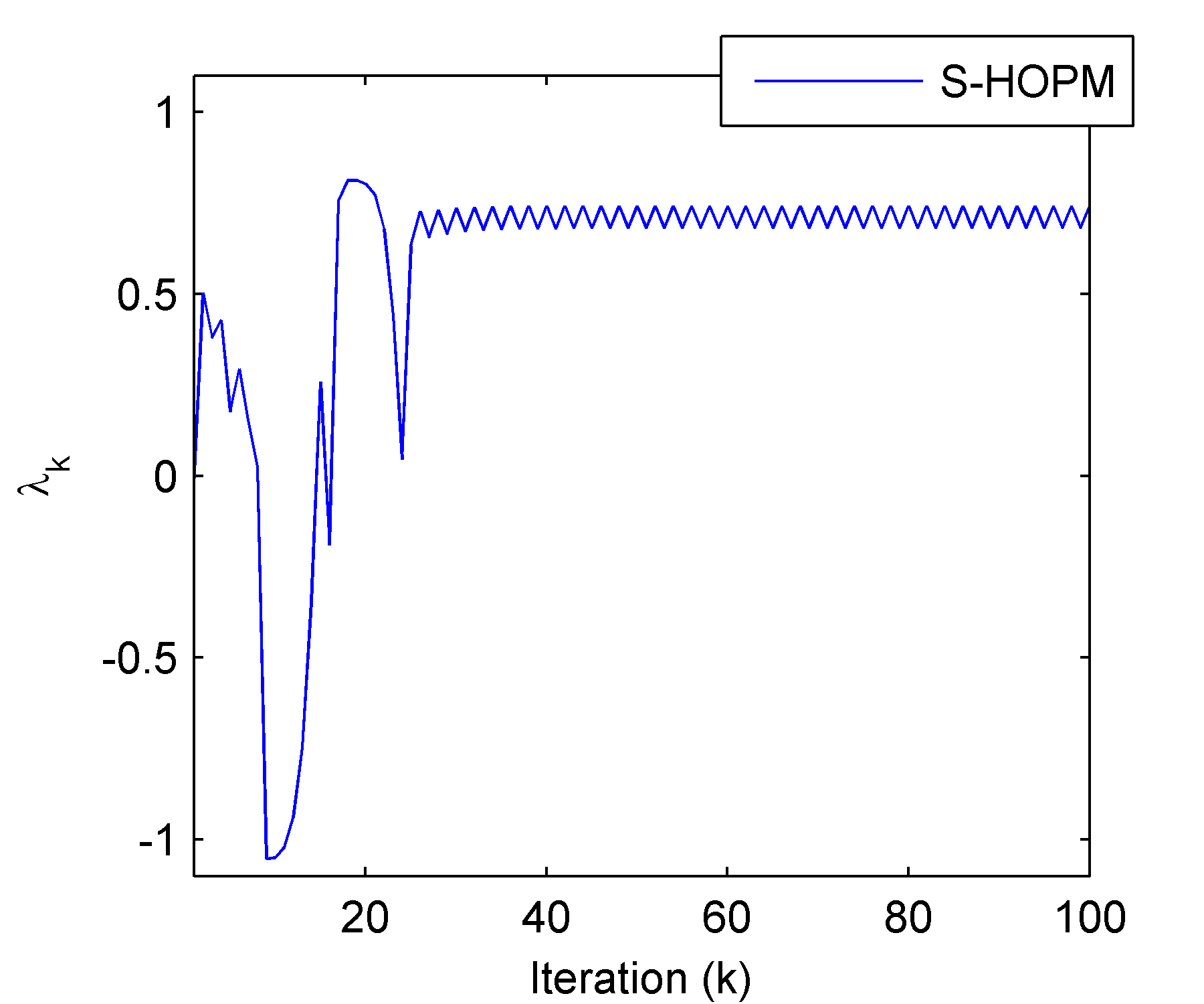
Kofidis and Regalia [11] observed that Algorithm 1 does not converge for this tensor. Because this problem is small, all eigenpairs can be calculated by Mathematica as described in §2.1. From Theorem 5.44, this problem has at most 13 eigenpairs; we list the 11 real eigenpairs in Table 1. We ran 100 trials of S-HOPM using different random starting points 𝐱0subscript𝐱0{\bm{\mathbf{{x}}}}_{0} chosen from a uniform distribution on [1,1]nsuperscript11𝑛[-1,1]^{n}. For these experiments, we allow up to 1000 iterations and say that the algorithm has converged if |λk+1λk|<1016subscript𝜆𝑘1subscript𝜆𝑘superscript1016|\lambda_{k+1}-\lambda_{k}|<10^{-16}. In every single trial for this tensor, the algorithm failed to converge. In Figure 1, we show an example {λk}subscript𝜆𝑘\{\lambda_{k}\} sequence with 𝐱0=[0.26950.19720.3370]Tsubscript𝐱0superscriptmatrix0.26950.19720.3370𝑇{\bm{\mathbf{{x}}}}_{0}=\begin{bmatrix}-0.2695&0.1972&0.3370\end{bmatrix}^{T}. This coincides with the results reported previously [11].   \square

Table 1: Eigenpairs for 𝓐[4,3]𝓐superscript43\bm{\mathscr{{A}}}\in\mathbb{R}^{[4,3]} from Example 3.23.
λ𝜆\lambda 𝐱Tsuperscript𝐱𝑇{\bm{\mathbf{{x}}}}^{T} Eigenvalues of C(λ,𝐱)𝐶𝜆𝐱C(\lambda,{\bm{\mathbf{{x}}}}) Type
0.88930.8893\phantom{-}0.8893 [ 0.66720.6672\phantom{-}0.6672 0.24710.2471\phantom{-}0.2471 0.70270.7027-0.7027 ] {{\{ 0.88570.8857-0.8857, 1.84591.8459-1.8459 }}\} Neg. stable
0.81690.8169\phantom{-}0.8169 [ 0.84120.8412\phantom{-}0.8412 0.26350.2635-0.2635 0.47220.4722\phantom{-}0.4722 ] {{\{ 0.90240.9024-0.9024, 2.25802.2580-2.2580 }}\} Neg. stable
0.51050.5105\phantom{-}0.5105 [ 0.35980.3598\phantom{-}0.3598 0.77800.7780-0.7780 0.51500.5150\phantom{-}0.5150 ] {{\{ 0.59400.5940\phantom{-}0.5940, 2.33982.3398-2.3398 }}\} Unstable
0.36330.3633\phantom{-}0.3633 [ 0.26760.2676\phantom{-}0.2676 0.64470.6447\phantom{-}0.6447 0.71600.7160\phantom{-}0.7160 ] {{\{ 1.17651.1765-1.1765, 0.57130.5713-0.5713 }}\} Neg. stable
0.26820.2682\phantom{-}0.2682 [ 0.60990.6099\phantom{-}0.6099 0.43620.4362\phantom{-}0.4362 0.66160.6616\phantom{-}0.6616 ] {{\{ 0.78520.7852\phantom{-}0.7852, 1.17931.1793-1.1793 }}\} Unstable
0.26280.2628\phantom{-}0.2628 [ 0.13180.1318\phantom{-}0.1318 0.44250.4425-0.4425 0.88700.8870-0.8870 ] {{\{ 0.61810.6181\phantom{-}0.6181, 2.17442.1744-2.1744 }}\} Unstable
0.24330.2433\phantom{-}0.2433 [ 0.98950.9895\phantom{-}0.9895 0.09470.0947\phantom{-}0.0947 0.10880.1088-0.1088 ] {{\{ 1.19421.1942-1.1942, 1.46271.4627\phantom{-}1.4627 }}\} Unstable
0.17350.1735\phantom{-}0.1735 [ 0.33570.3357\phantom{-}0.3357 0.90730.9073\phantom{-}0.9073 0.25310.2531\phantom{-}0.2531 ] {{\{ 1.09661.0966-1.0966, 0.86290.8629\phantom{-}0.8629 }}\} Unstable
0.04510.0451-0.0451 [ 0.77970.7797\phantom{-}0.7797 0.61350.6135\phantom{-}0.6135 0.12500.1250\phantom{-}0.1250 ] {{\{ 0.82090.8209\phantom{-}0.8209, 1.24561.2456\phantom{-}1.2456 }}\} Pos. stable
0.56290.5629-0.5629 [ 0.17620.1762\phantom{-}0.1762 0.17960.1796-0.1796 0.96780.9678\phantom{-}0.9678 ] {{\{ 1.62871.6287\phantom{-}1.6287, 2.38222.3822\phantom{-}2.3822 }}\} Pos. stable
1.09541.0954-1.0954 [ 0.59150.5915\phantom{-}0.5915 0.74670.7467-0.7467 0.30430.3043-0.3043 ] {{\{ 1.86281.8628\phantom{-}1.8628, 2.74692.7469\phantom{-}2.7469 }}\} Pos. stable
Refer to caption
Fig. 1: Example λksubscript𝜆𝑘\lambda_{k} values for S-HOPM on 𝓐[4,3]𝓐superscript43\bm{\mathscr{{A}}}\in\mathbb{R}^{[4,3]} from Example 3.23.
Example 3.24.

As a second illustrative example, we consider an odd-order tensor 𝓐[3,3]𝓐superscript33\bm{\mathscr{{A}}}\in\mathbb{R}^{[3,3]} defined by

a111subscript𝑎111\displaystyle a_{111} =0.1281,absent0.1281\displaystyle=-0.1281, a112subscript𝑎112\displaystyle a_{112} =0.0516,absent0.0516\displaystyle=\phantom{-}0.0516, a113subscript𝑎113\displaystyle a_{113} =0.0954,absent0.0954\displaystyle=-0.0954, a122subscript𝑎122\displaystyle a_{122} =0.1958,absent0.1958\displaystyle=-0.1958,
a123subscript𝑎123\displaystyle a_{123} =0.1790,absent0.1790\displaystyle=-0.1790, a133subscript𝑎133\displaystyle a_{133} =0.2676,absent0.2676\displaystyle=-0.2676, a222subscript𝑎222\displaystyle a_{222} =0.3251,absent0.3251\displaystyle=\phantom{-}0.3251, a223subscript𝑎223\displaystyle a_{223} =0.2513,absent0.2513\displaystyle=\phantom{-}0.2513,
a233subscript𝑎233\displaystyle a_{233} =0.1773,absent0.1773\displaystyle=\phantom{-}0.1773, a333subscript𝑎333\displaystyle a_{333} =0.0338.absent0.0338\displaystyle=\phantom{-}0.0338.

From Theorem 5.44, 𝓐𝓐\bm{\mathscr{{A}}} has at most 7 eigenpairs; in this case we achieve that bound and the eigenpairs are listed in Table 2. We ran 100 trials of S-HOPM as described for Example 3.23. Every trial converged to either λ=0.8730𝜆0.8730\lambda=0.8730 or λ=0.4306𝜆0.4306\lambda=0.4306, as summarized in Table 3. Therefore, S-HOPM finds 2 of the 7 possible eigenvalues.

Table 2: Eigenpairs for 𝓐[3,3]𝓐superscript33\bm{\mathscr{{A}}}\in\mathbb{R}^{[3,3]} from Example 3.24.
λ𝜆\lambda 𝐱Tsuperscript𝐱𝑇{\bm{\mathbf{{x}}}}^{T} Eigenvalues of C(λ,𝐱)𝐶𝜆𝐱C(\lambda,{\bm{\mathbf{{x}}}}) Type
0.87300.87300.8730 [ 0.39220.3922-0.3922 0.72490.7249\phantom{-}0.7249 0.56640.5664\phantom{-}0.5664 ] {{\{ 1.12931.1293-1.1293, 0.88070.8807-0.8807 }}\} Neg. stable
0.43060.43060.4306 [ 0.71870.7187-0.7187 0.12450.1245-0.1245 0.68400.6840-0.6840 ] {{\{ 0.44200.4420-0.4420, 0.82750.8275-0.8275 }}\} Neg. stable
0.22940.22940.2294 [ 0.84460.8446-0.8446 0.43860.4386\phantom{-}0.4386 0.30700.3070-0.3070 ] {{\{ 0.26410.2641-0.2641, 0.71510.7151\phantom{-}0.7151 }}\} Unstable
0.01800.01800.0180 [ 0.71320.7132\phantom{-}0.7132 0.50930.5093\phantom{-}0.5093 0.48170.4817-0.4817 ] {{\{ 0.40210.4021-0.4021, 0.13200.1320-0.1320 }}\} Neg. stable
0.00330.00330.0033 [ 0.44770.4477\phantom{-}0.4477 0.77400.7740\phantom{-}0.7740 0.44780.4478-0.4478 ] {{\{ 0.10110.1011-0.1011, 0.24610.2461\phantom{-}0.2461 }}\} Unstable
0.00180.00180.0018 [ 0.33050.3305\phantom{-}0.3305 0.63140.6314\phantom{-}0.6314 0.70150.7015-0.7015 ] {{\{ 0.15920.1592\phantom{-}0.1592, 0.12410.1241-0.1241 }}\} Unstable
0.00060.00060.0006 [ 0.29070.2907\phantom{-}0.2907 0.73590.7359\phantom{-}0.7359 0.61150.6115-0.6115 ] {{\{ 0.14050.1405\phantom{-}0.1405, 0.09680.0968\phantom{-}0.0968 }}\} Pos. stable
Table 3: Eigenpairs for 𝓐[3,3]𝓐superscript33\bm{\mathscr{{A}}}\in\mathbb{R}^{[3,3]} from Example 3.24 computed by S-HOPM with 100 random starts.
# Occurrences λ𝜆\lambda 𝐱𝐱{\bm{\mathbf{{x}}}} Median Its.
62 0.87300.8730\phantom{-}0.8730 [ 0.39220.3922-0.3922 0.72490.7249\phantom{-}0.7249 0.56640.5664\phantom{-}0.5664 ] 19
38 0.43060.4306\phantom{-}0.4306 [ 0.71870.7187-0.7187 0.12450.1245-0.1245 0.68400.6840-0.6840 ] 184

In their analysis, Kofidis and Regalia [11] proved that the sequence {λk}subscript𝜆𝑘\{\lambda_{k}\} in Algorithm 1 converges if 𝓐[m,n]𝓐superscript𝑚𝑛\bm{\mathscr{{A}}}\in\mathbb{R}^{[m,n]} is even-order and the function f(𝐱)𝑓𝐱f({\bm{\mathbf{{x}}}}) is convex or concave on nsuperscript𝑛\mathbb{R}^{n}. Since m=2𝑚2m=2\ell (because m𝑚m is even), f𝑓f can be expressed as

f(𝐱)=(𝐱𝐱 times)T𝐀(𝐱𝐱 times),𝑓𝐱superscriptsubscripttensor-product𝐱𝐱 times𝑇𝐀subscripttensor-product𝐱𝐱 timesf({\bm{\mathbf{{x}}}})=(\,\underbrace{{\bm{\mathbf{{x}}}}\otimes\cdots\otimes{\bm{\mathbf{{x}}}}}_{\text{$\ell$ times}}\,)^{T}{\bm{\mathbf{{A}}}}\,(\,\underbrace{{\bm{\mathbf{{x}}}}\otimes\cdots\otimes{\bm{\mathbf{{x}}}}}_{\text{$\ell$ times}}\,),

where 𝐀n×n𝐀superscriptsuperscript𝑛superscript𝑛{\bm{\mathbf{{A}}}}\in\mathbb{R}^{n^{\ell}\times n^{\ell}} is an unfolded version of the tensor 𝓐𝓐\bm{\mathscr{{A}}}.222Specifically, 𝐀𝐀(×𝒞)𝐀subscript𝐀𝒞{\bm{\mathbf{{A}}}}\equiv{\bm{\mathbf{{A}}}}_{(\mathcal{R}\times\mathcal{C})} with ={1,,}1\mathcal{R}=\{1,\dots,\ell\} and 𝒞={+1,,m}𝒞1𝑚\mathcal{C}=\{\ell+1,\dots,m\} in matricization notation [12]. Since 𝓐𝓐\bm{\mathscr{{A}}} is symmetric, it follows that 𝐀𝐀{\bm{\mathbf{{A}}}} is symmetric. The condition that f𝑓f is convex (concave) is satisfied if the Hessian

2f(𝐱)=(𝐈𝐱𝐱1 times)T𝐀(𝐈𝐱𝐱1 times)superscript2𝑓𝐱superscripttensor-product𝐈subscripttensor-product𝐱𝐱1 times𝑇𝐀tensor-product𝐈subscripttensor-product𝐱𝐱1 times\nabla^{2}f({\bm{\mathbf{{x}}}})=(\,{\bm{\mathbf{{I}}}}\otimes\underbrace{{\bm{\mathbf{{x}}}}\otimes\cdots\otimes{\bm{\mathbf{{x}}}}}_{\text{$\ell-1$ times}}\,)^{T}{\bm{\mathbf{{A}}}}\,(\,{\bm{\mathbf{{I}}}}\otimes\underbrace{{\bm{\mathbf{{x}}}}\otimes\cdots\otimes{\bm{\mathbf{{x}}}}}_{\text{$\ell-1$ times}}\,)

is positive (negative) semidefinite for all 𝐱n𝐱superscript𝑛{\bm{\mathbf{{x}}}}\in\mathbb{R}^{n}.

We make a few notes regarding these results. First, even though f𝑓f is convex, its restriction to the nonconvex set ΣΣ\Sigma is not. Second, {λk}subscript𝜆𝑘\{\lambda_{k}\} is increasing if f𝑓f is convex and decreasing if f𝑓f is concave. Third, only {λk}subscript𝜆𝑘\{\lambda_{k}\} is proved to converge for S-HOPM [11, Theorem 4]; the iterates {𝐱k}subscript𝐱𝑘\{{\bm{\mathbf{{x}}}}_{k}\} may not. In particular, it is easy to observe that the sign of 𝐱ksubscript𝐱𝑘{\bm{\mathbf{{x}}}}_{k} may flip back and forth if the concave case is not handled correctly.

4 Shifted symmetric higher-order power method (SS-HOPM)

In this section, we show that S-HOPM can be modified by adding a “shift” that guarantees that the method will always converge to an eigenpair. In the context of ICA, this idea has also been proposed by Regalia and Kofidis [23] and Erdogen [8]. Based on the observation that S-HOPM is guaranteed to converge if the underlying function is convex or concave on nsuperscript𝑛\mathbb{R}^{n}, our method works with a suitably modified function

f^(𝐱)f(𝐱)+α(𝐱T𝐱)m/2.^𝑓𝐱𝑓𝐱𝛼superscriptsuperscript𝐱𝑇𝐱𝑚2\hat{f}({\bm{\mathbf{{x}}}})\equiv f({\bm{\mathbf{{x}}}})+\alpha({\bm{\mathbf{{x}}}}^{T}{\bm{\mathbf{{x}}}})^{m/2}. (11)

Maximizing f^^𝑓\hat{f} on ΣΣ\Sigma is the same as maximizing f𝑓f plus a constant, yet the properties of the modified function force convexity or concavity and consequently guarantee convergence to a KKT point (not necessary the global maximum or minimum). Note that previous papers [23, 8] have proposed similar shifted functions that are essentially of the form f^(𝐱)f(𝐱)+α𝐱T𝐱,^𝑓𝐱𝑓𝐱𝛼superscript𝐱𝑇𝐱\hat{f}({\bm{\mathbf{{x}}}})\equiv f({\bm{\mathbf{{x}}}})+\alpha{\bm{\mathbf{{x}}}}^{T}{\bm{\mathbf{{x}}}}, differing only in the exponent.

An advantage of our choice of f^^𝑓\hat{f} in (11) is that, for even m𝑚m, it can be interpreted as

f^(𝐱)=𝓐^𝐱m(𝓐+α𝓔)𝐱m,^𝑓𝐱^𝓐superscript𝐱𝑚𝓐𝛼𝓔superscript𝐱𝑚\hat{f}({\bm{\mathbf{{x}}}})=\hat{\bm{\mathscr{{A}}}}{\bm{\mathbf{{x}}}}^{m}\equiv(\bm{\mathscr{{A}}}+\alpha\bm{\mathscr{{E}}}){\bm{\mathbf{{x}}}}^{m},

where 𝓔𝓔\bm{\mathscr{{E}}} is the identity tensor as defined in (4). Thus, for even m𝑚m, our proposed method can be interpreted as S-HOPM applied to a modified tensor that directly satisfies the convexity properties to guarantee convergence [11]. Because 𝓔𝐱m1=𝐱𝓔superscript𝐱𝑚1𝐱\bm{\mathscr{{E}}}{\bm{\mathbf{{x}}}}^{m-1}={\bm{\mathbf{{x}}}} for 𝐱Σ𝐱Σ{\bm{\mathbf{{x}}}}\in\Sigma, the eigenvectors of 𝓐^^𝓐\hat{\bm{\mathscr{{A}}}} are the same as those of 𝓐𝓐\bm{\mathscr{{A}}} and the eigenvalues are shifted by α𝛼\alpha. Our results, however, are for both odd- and even-order tensors.

Algorithm 2 presents the shifted symmetric higher-order power method (SS-HOPM). Without loss of generality, we assume that a positive shift (α0𝛼0\alpha\geq 0) is used to make the modified function in (11) convex and a negative shift (α<0𝛼0\alpha<0) to make it concave. We have two key results. Theorem 4.31 shows that for any starting point 𝐱0Σsubscript𝐱0Σ{\bm{\mathbf{{x}}}}_{0}\in\Sigma, the sequence {λk}subscript𝜆𝑘\{\lambda_{k}\} produced by Algorithm 2 is guaranteed to converge to an eigenvalue in the convex case if

α>β(𝓐)(m1)max𝐱Σρ(𝓐𝐱m2).𝛼𝛽𝓐𝑚1subscript𝐱Σ𝜌𝓐superscript𝐱𝑚2\alpha>\beta(\bm{\mathscr{{A}}})\equiv(m-1)\cdot\max_{{\bm{\mathbf{{x}}}}\in\Sigma}\rho(\bm{\mathscr{{A}}}{\bm{\mathbf{{x}}}}^{m-2}). (12)

Corollary 4.34 handles the concave case where we require α<β(𝓐)𝛼𝛽𝓐\alpha<-\beta(\bm{\mathscr{{A}}}). Theorem 4.37 further shows that Algorithm 2 in the convex case will generically converge to an eigenpair (λ,𝐱)𝜆𝐱(\lambda,{\bm{\mathbf{{x}}}}) that is negative stable. Corollary 4.39 proves that Algorithm 2 in the concave case will generically converge to an eigenpair that is positive stable. Generally, neither version will converge to an eigenpair that is unstable.

Algorithm 2 Shifted Symmetric Higher-Order Power Method (SS-HOPM)

Given a tensor 𝓐[m,n]𝓐superscript𝑚𝑛\bm{\mathscr{{A}}}\in\mathbb{R}^{[m,n]}.

1:𝐱0nsubscript𝐱0superscript𝑛{\bm{\mathbf{{x}}}}_{0}\in\mathbb{R}^{n} with 𝐱0=1normsubscript𝐱01\|{\bm{\mathbf{{x}}}}_{0}\|=1. Let λ0=𝓐𝐱0msubscript𝜆0𝓐superscriptsubscript𝐱0𝑚\lambda_{0}=\bm{\mathscr{{A}}}{\bm{\mathbf{{x}}}}_{0}^{m}.
2:α𝛼\alpha\in\mathbb{R}
3:for k=0,1,𝑘01k=0,1,\dots do
4:     if α0𝛼0\alpha\geq 0 then
5:         𝐱^k+1𝓐𝐱km1+α𝐱ksubscript^𝐱𝑘1𝓐superscriptsubscript𝐱𝑘𝑚1𝛼subscript𝐱𝑘\hat{\bm{\mathbf{{x}}}}_{k+1}\leftarrow\bm{\mathscr{{A}}}{\bm{\mathbf{{x}}}}_{k}^{m-1}+\alpha{\bm{\mathbf{{x}}}}_{k} \triangleright Assumed Convex
6:     else
7:         𝐱^k+1(𝓐𝐱km1+α𝐱k)subscript^𝐱𝑘1𝓐superscriptsubscript𝐱𝑘𝑚1𝛼subscript𝐱𝑘\hat{\bm{\mathbf{{x}}}}_{k+1}\leftarrow-(\bm{\mathscr{{A}}}{\bm{\mathbf{{x}}}}_{k}^{m-1}+\alpha{\bm{\mathbf{{x}}}}_{k}) \triangleright Assumed Concave
8:     end if
9:     𝐱k+1𝐱^k+1/𝐱^k+1subscript𝐱𝑘1subscript^𝐱𝑘1normsubscript^𝐱𝑘1{\bm{\mathbf{{x}}}}_{k+1}\leftarrow\hat{\bm{\mathbf{{x}}}}_{k+1}/\|\hat{\bm{\mathbf{{x}}}}_{k+1}\|
10:     λk+1𝓐𝐱k+1msubscript𝜆𝑘1𝓐superscriptsubscript𝐱𝑘1𝑚\lambda_{k+1}\leftarrow\bm{\mathscr{{A}}}{\bm{\mathbf{{x}}}}_{k+1}^{m}
11:end for

4.1 SS-HOPM convergence analysis

We first establish a few key lemmas that guide the choice of the shift α>β(𝓐)𝛼𝛽𝓐\alpha>\beta(\bm{\mathscr{{A}}}) in SS-HOPM.

Lemma 4.25.

Let 𝓐[m,n]𝓐superscript𝑚𝑛\bm{\mathscr{{A}}}\in\mathbb{R}^{[m,n]} be symmetric and let β(𝓐)𝛽𝓐\beta(\bm{\mathscr{{A}}}) be as defined in (12). Then β(𝓐)(m1)i1,,im|ai1im|𝛽𝓐𝑚1subscriptsubscript𝑖1subscript𝑖𝑚subscript𝑎subscript𝑖1subscript𝑖𝑚\beta(\bm{\mathscr{{A}}})\leq(m-1)\sum_{i_{1},\dots,i_{m}}|{a}_{i_{1}\dots i_{m}}|.

Proof 4.26.

For all 𝐱,𝐲Σ𝐱𝐲Σ{\bm{\mathbf{{x}}}},{\bm{\mathbf{{y}}}}\in\Sigma, we obtain |𝐲T(𝓐𝐱m2)𝐲|i1,,im|ai1im|superscript𝐲𝑇𝓐superscript𝐱𝑚2𝐲subscriptsubscript𝑖1subscript𝑖𝑚subscript𝑎subscript𝑖1subscript𝑖𝑚|{\bm{\mathbf{{y}}}}^{T}(\bm{\mathscr{{A}}}{\bm{\mathbf{{x}}}}^{m-2}){\bm{\mathbf{{y}}}}|\leq\sum_{i_{1},\dots,i_{m}}|{a}_{i_{1}\dots i_{m}}| by applying the triangle inequality to the sum of nmsuperscript𝑛𝑚n^{m} terms. Thus ρ(𝓐𝐱m2)i1,,im|ai1im|𝜌𝓐superscript𝐱𝑚2subscriptsubscript𝑖1subscript𝑖𝑚subscript𝑎subscript𝑖1subscript𝑖𝑚\rho(\bm{\mathscr{{A}}}{\bm{\mathbf{{x}}}}^{m-2})\leq\sum_{i_{1},\dots,i_{m}}|{a}_{i_{1}\dots i_{m}}| for all 𝐱Σ𝐱Σ{\bm{\mathbf{{x}}}}\in\Sigma, and the result follows.

Lemma 4.27.

Let 𝓐[m,n]𝓐superscript𝑚𝑛\bm{\mathscr{{A}}}\in\mathbb{R}^{[m,n]} be symmetric, let f(𝐱)=𝓐𝐱m𝑓𝐱𝓐superscript𝐱𝑚f({\bm{\mathbf{{x}}}})=\bm{\mathscr{{A}}}{\bm{\mathbf{{x}}}}^{m}, and let β(𝓐)𝛽𝓐\beta(\bm{\mathscr{{A}}}) be as defined in (12). Then |f(𝐱)|β(𝓐)/(m1)𝑓𝐱𝛽𝓐𝑚1|f({\bm{\mathbf{{x}}}})|\leq\beta(\bm{\mathscr{{A}}})/(m-1) for all 𝐱Σ𝐱Σ{\bm{\mathbf{{x}}}}\in\Sigma.

Proof 4.28.

We have |𝓐𝐱m|=|𝐱T(𝓐𝐱m2)𝐱|ρ(𝓐𝐱m2)β(𝓐)/(m1)𝓐superscript𝐱𝑚superscript𝐱𝑇𝓐superscript𝐱𝑚2𝐱𝜌𝓐superscript𝐱𝑚2𝛽𝓐𝑚1|\bm{\mathscr{{A}}}{\bm{\mathbf{{x}}}}^{m}|=|{\bm{\mathbf{{x}}}}^{T}(\bm{\mathscr{{A}}}{\bm{\mathbf{{x}}}}^{m-2}){\bm{\mathbf{{x}}}}|\leq\rho(\bm{\mathscr{{A}}}{\bm{\mathbf{{x}}}}^{m-2})\leq\beta(\bm{\mathscr{{A}}})/(m-1).

The preceding lemma upper bounds the magnitude of any eigenvalue of 𝓐𝓐\bm{\mathscr{{A}}} by β(𝓐)/(m1)𝛽𝓐𝑚1\beta(\bm{\mathscr{{A}}})/(m-1) since any eigenpair (λ,𝐱)𝜆𝐱(\lambda,{\bm{\mathbf{{x}}}}) satisfies λ=f(𝐱)𝜆𝑓𝐱\lambda=f({\bm{\mathbf{{x}}}}). Thus, choosing α>β(𝓐)𝛼𝛽𝓐\alpha>\beta(\bm{\mathscr{{A}}}) implies that α𝛼\alpha is greater than the magnitude of any eigenvalue of 𝓐𝓐\bm{\mathscr{{A}}}.

Lemma 4.29.

Let 𝓐[m,n]𝓐superscript𝑚𝑛\bm{\mathscr{{A}}}\in\mathbb{R}^{[m,n]} be symmetric and let H(𝐱)𝐻𝐱H({\bm{\mathbf{{x}}}}) and β(𝓐)𝛽𝓐\beta(\bm{\mathscr{{A}}}) be as defined in (9) and (12). Then ρ(H(𝐱))mβ(𝓐)𝜌𝐻𝐱𝑚𝛽𝓐\rho(H({\bm{\mathbf{{x}}}}))\leq m\beta(\bm{\mathscr{{A}}}) for all 𝐱Σ𝐱Σ{\bm{\mathbf{{x}}}}\in\Sigma.

Proof 4.30.

This follows directly from (9) and (12).

The following theorem proves that Algorithm 2 will always converge. Choosing α>(m1)i1,,im|ai1im|𝛼𝑚1subscriptsubscript𝑖1subscript𝑖𝑚subscript𝑎subscript𝑖1subscript𝑖𝑚\alpha>(m-1)\sum_{i_{1},\dots,i_{m}}|{a}_{i_{1}\dots i_{m}}| is a conservative choice that is guaranteed to work by Lemma 4.25, but this may slow down convergence considerably, as we show in subsequent analysis and examples.

Theorem 4.31.

Let 𝓐[m,n]𝓐superscript𝑚𝑛\bm{\mathscr{{A}}}\in\mathbb{R}^{[m,n]} be symmetric. For α>β(𝓐)𝛼𝛽𝓐\alpha>\beta(\bm{\mathscr{{A}}}), where β(𝓐)𝛽𝓐\beta(\bm{\mathscr{{A}}}) is defined in (12), the iterates {λk,𝐱k}subscript𝜆𝑘subscript𝐱𝑘\{\lambda_{k},{\bm{\mathbf{{x}}}}_{k}\} produced by Algorithm 2 satisfy the following properties. (a) The sequence {λk}subscript𝜆𝑘\{\lambda_{k}\} is nondecreasing, and there exists λsubscript𝜆\lambda_{*} such that λkλsubscript𝜆𝑘subscript𝜆\lambda_{k}\rightarrow\lambda_{*}. (b) The sequence {𝐱k}subscript𝐱𝑘\{{\bm{\mathbf{{x}}}}_{k}\} has an accumulation point. (c) For every such accumulation point 𝐱subscript𝐱{\bm{\mathbf{{x}}}}_{*}, the pair (λ,𝐱)subscript𝜆subscript𝐱(\lambda_{*},{\bm{\mathbf{{x}}}}_{*}) is an eigenpair of 𝓐𝓐\bm{\mathscr{{A}}}. (d) If 𝓐𝓐\bm{\mathscr{{A}}} has finitely many real eigenvectors, then there exists 𝐱subscript𝐱{\bm{\mathbf{{x}}}}_{*} such that 𝐱k𝐱subscript𝐱𝑘subscript𝐱{\bm{\mathbf{{x}}}}_{k}\rightarrow{\bm{\mathbf{{x}}}}_{*}.

Proof 4.32.

Our analysis depends on the modified function f^^𝑓\hat{f} defined in (11). Its gradient and Hessian for 𝐱𝟎𝐱0{\bm{\mathbf{{x}}}}\neq{\bm{\mathbf{{0}}}} are

g^(𝐱)^𝑔𝐱\displaystyle\hat{g}({\bm{\mathbf{{x}}}}) f^(𝐱)=g(𝐱)+mα(𝐱T𝐱)m/21𝐱,absent^𝑓𝐱𝑔𝐱𝑚𝛼superscriptsuperscript𝐱𝑇𝐱𝑚21𝐱\displaystyle\equiv\nabla\hat{f}({\bm{\mathbf{{x}}}})=g({\bm{\mathbf{{x}}}})+m\alpha({\bm{\mathbf{{x}}}}^{T}{\bm{\mathbf{{x}}}})^{m/2-1}{\bm{\mathbf{{x}}}}, (13)
H^(𝐱)^𝐻𝐱\displaystyle\hat{H}({\bm{\mathbf{{x}}}}) 2f^(𝐱)=H(𝐱)+mα(𝐱T𝐱)m/21𝐈+m(m2)α(𝐱T𝐱)m/22𝐱𝐱T,absentsuperscript2^𝑓𝐱𝐻𝐱𝑚𝛼superscriptsuperscript𝐱𝑇𝐱𝑚21𝐈𝑚𝑚2𝛼superscriptsuperscript𝐱𝑇𝐱𝑚22superscript𝐱𝐱𝑇\displaystyle\equiv\nabla^{2}\hat{f}({\bm{\mathbf{{x}}}})=H({\bm{\mathbf{{x}}}})+m\alpha({\bm{\mathbf{{x}}}}^{T}{\bm{\mathbf{{x}}}})^{m/2-1}{\bm{\mathbf{{I}}}}+m(m-2)\alpha({\bm{\mathbf{{x}}}}^{T}{\bm{\mathbf{{x}}}})^{m/2-2}{\bm{\mathbf{{x}}}}{\bm{\mathbf{{x}}}}^{T}, (14)

where g𝑔g and H𝐻H are the gradient and Hessian of f𝑓f from Lemma 3.16 and Lemma 3.20, respectively. And because f^(𝐱)=O(𝐱m)^𝑓𝐱𝑂superscriptnorm𝐱𝑚\hat{f}({\bm{\mathbf{{x}}}})=O(\|{\bm{\mathbf{{x}}}}\|^{m}), as 𝐱𝟎𝐱0{\bm{\mathbf{{x}}}}\to{\bm{\mathbf{{0}}}}, it follows that f^(𝐱)^𝑓𝐱\hat{f}({\bm{\mathbf{{x}}}}) is of third or higher order in 𝐱𝐱{\bm{\mathbf{{x}}}} for m3𝑚3m\geq 3; thus g^(𝟎)=𝟎^𝑔00\hat{g}({\bm{\mathbf{{0}}}})={\bm{\mathbf{{0}}}} and H^(𝟎)=𝟎^𝐻00\hat{H}({\bm{\mathbf{{0}}}})={\bm{\mathbf{{0}}}}.

Because it is important for the entire proof, we first show that f^^𝑓\hat{f} is convex on nsuperscript𝑛\mathbb{R}^{n} for α>β(𝓐)𝛼𝛽𝓐\alpha>\beta(\bm{\mathscr{{A}}}). As noted, if 𝐱=𝟎𝐱0{\bm{\mathbf{{x}}}}={\bm{\mathbf{{0}}}}, we have H^(𝐱)=𝟎^𝐻𝐱0\hat{H}({\bm{\mathbf{{x}}}})={\bm{\mathbf{{0}}}} for m3𝑚3m\geq 3. Consider nonzero 𝐱n𝐱superscript𝑛{\bm{\mathbf{{x}}}}\in\mathbb{R}^{n} and define 𝐱¯=𝐱/𝐱Σ¯𝐱𝐱norm𝐱Σ\bar{\bm{\mathbf{{x}}}}={\bm{\mathbf{{x}}}}/\|{\bm{\mathbf{{x}}}}\|\in\Sigma; then H^(𝐱)^𝐻𝐱\hat{H}({\bm{\mathbf{{x}}}}) is positive semidefinite (in fact, positive definite) by Lemma 4.29 since

𝐲TH^(𝐱)𝐲superscript𝐲𝑇^𝐻𝐱𝐲\displaystyle{\bm{\mathbf{{y}}}}^{T}\hat{H}({\bm{\mathbf{{x}}}}){\bm{\mathbf{{y}}}} =𝐱m2(𝐲TH(𝐱¯)𝐲+mα+m(m1)α(𝐱¯T𝐲)2)absentsuperscriptnorm𝐱𝑚2superscript𝐲𝑇𝐻¯𝐱𝐲𝑚𝛼𝑚𝑚1𝛼superscriptsuperscript¯𝐱𝑇𝐲2\displaystyle=\|{\bm{\mathbf{{x}}}}\|^{m-2}\left({\bm{\mathbf{{y}}}}^{T}H(\bar{\bm{\mathbf{{x}}}}){\bm{\mathbf{{y}}}}+m\alpha+m(m-1)\alpha(\bar{\bm{\mathbf{{x}}}}^{T}{\bm{\mathbf{{y}}}})^{2}\right)
𝐱m2(mβ(𝓐)+mα+0)>0for all𝐲Σ.formulae-sequenceabsentsuperscriptnorm𝐱𝑚2𝑚𝛽𝓐𝑚𝛼00for all𝐲Σ\displaystyle\geq\|{\bm{\mathbf{{x}}}}\|^{m-2}\left(-m\beta(\bm{\mathscr{{A}}})+m\alpha+0\right)>0\quad\text{for all}\quad{\bm{\mathbf{{y}}}}\in\Sigma.

By Property 2.8, f^^𝑓\hat{f} is convex on nsuperscript𝑛\mathbb{R}^{n} because its Hessian is positive semidefinite.

We also note that α𝛼-\alpha must be an eigenvalue of 𝓐𝓐\bm{\mathscr{{A}}} if g^(𝐱)=𝟎^𝑔𝐱0\hat{g}({\bm{\mathbf{{x}}}})={\bm{\mathbf{{0}}}} for some 𝐱Σ𝐱Σ{\bm{\mathbf{{x}}}}\in\Sigma, since

g^(𝐱)=𝟎implies𝓐𝐱m1+α𝐱=𝟎.formulae-sequence^𝑔𝐱0implies𝓐superscript𝐱𝑚1𝛼𝐱0\hat{g}({\bm{\mathbf{{x}}}})={\bm{\mathbf{{0}}}}\quad\text{implies}\quad\bm{\mathscr{{A}}}{\bm{\mathbf{{x}}}}^{m-1}+\alpha{\bm{\mathbf{{x}}}}={\bm{\mathbf{{0}}}}.

By Lemma 4.27, choosing α>β(𝓐)𝛼𝛽𝓐\alpha>\beta(\bm{\mathscr{{A}}}) ensures that α𝛼\alpha is greater than the magnitude of any eigenvalue, and so g^(𝐱)𝟎^𝑔𝐱0\hat{g}({\bm{\mathbf{{x}}}})\neq{\bm{\mathbf{{0}}}} for all 𝐱Σ𝐱Σ{\bm{\mathbf{{x}}}}\in\Sigma. This ensures that the update in Algorithm 2, which reduces to

𝐱k+1=g^(𝐱k)g^(𝐱k)subscript𝐱𝑘1^𝑔subscript𝐱𝑘norm^𝑔subscript𝐱𝑘{\bm{\mathbf{{x}}}}_{k+1}=\frac{\hat{g}({\bm{\mathbf{{x}}}}_{k})}{\|\hat{g}({\bm{\mathbf{{x}}}}_{k})\|} (15)

in the convex case, is always well defined.

  1. (a)

    Since f^^𝑓\hat{f} is convex on ΓΓ\Gamma and 𝐱k+1,𝐱kΣsubscript𝐱𝑘1subscript𝐱𝑘Σ{\bm{\mathbf{{x}}}}_{k+1},{\bm{\mathbf{{x}}}}_{k}\in\Sigma and 𝐱k+1=f^(𝐱k)/f^(𝐱k)subscript𝐱𝑘1^𝑓subscript𝐱𝑘norm^𝑓subscript𝐱𝑘{\bm{\mathbf{{x}}}}_{k+1}=\nabla\hat{f}({\bm{\mathbf{{x}}}}_{k})/\|\nabla\hat{f}({\bm{\mathbf{{x}}}}_{k})\|, Theorem 2.9 yields

    λk+1λk=f^(𝐱k+1)f^(𝐱k)0,subscript𝜆𝑘1subscript𝜆𝑘^𝑓subscript𝐱𝑘1^𝑓subscript𝐱𝑘0\lambda_{k+1}-\lambda_{k}=\hat{f}({\bm{\mathbf{{x}}}}_{k+1})-\hat{f}({\bm{\mathbf{{x}}}}_{k})\geq 0,

    where the nonstrict inequality covers the possibility that 𝐱k+1=𝐱ksubscript𝐱𝑘1subscript𝐱𝑘{\bm{\mathbf{{x}}}}_{k+1}={\bm{\mathbf{{x}}}}_{k}. Thus, {λk}subscript𝜆𝑘\{\lambda_{k}\} is a nondecreasing sequence. By Lemma 4.27, λk=f(𝐱k)subscript𝜆𝑘𝑓subscript𝐱𝑘\lambda_{k}=f({\bm{\mathbf{{x}}}}_{k}) is bounded, so the sequence must converge to a limit point λsubscript𝜆\lambda_{*}.333Note that the similar approach proposed for ICA [23, Theorem 2] allows the shift α𝛼\alpha to vary at each iteration so long as the underlying function remains convex.

  2. (b)

    Since {𝐱k}subscript𝐱𝑘\{{\bm{\mathbf{{x}}}}_{k}\} is an infinite sequence on a compact set ΣΣ\Sigma, it must have an accumulation point 𝐱Σsubscript𝐱Σ{\bm{\mathbf{{x}}}}_{*}\in\Sigma by the Bolzano-Weierstrass theorem. Note also that continuity of f𝑓f implies that λ=𝓐𝐱msubscript𝜆𝓐superscriptsubscript𝐱𝑚\lambda_{*}=\bm{\mathscr{{A}}}{\bm{\mathbf{{x}}}}_{*}^{m}.

  3. (c)

    By part (a) of the proof, convexity of f^^𝑓\hat{f}, and Property 2.7, we have

    f^(𝐱k+1)f^(𝐱k)0^𝑓subscript𝐱𝑘1^𝑓subscript𝐱𝑘0\hat{f}({\bm{\mathbf{{x}}}}_{k+1})-\hat{f}({\bm{\mathbf{{x}}}}_{k})\rightarrow 0

    and thus

    g^(𝐱k)T(𝐱k+1𝐱k)0.^𝑔superscriptsubscript𝐱𝑘𝑇subscript𝐱𝑘1subscript𝐱𝑘0\hat{g}({\bm{\mathbf{{x}}}}_{k})^{T}({\bm{\mathbf{{x}}}}_{k+1}-{\bm{\mathbf{{x}}}}_{k})\rightarrow 0.

    Using (15), we can rewrite the above formula as

    g^(𝐱k)g^(𝐱k)T𝐱k0.norm^𝑔subscript𝐱𝑘^𝑔superscriptsubscript𝐱𝑘𝑇subscript𝐱𝑘0\|\hat{g}({\bm{\mathbf{{x}}}}_{k})\|-\hat{g}({\bm{\mathbf{{x}}}}_{k})^{T}{\bm{\mathbf{{x}}}}_{k}\rightarrow 0. (16)

    By continuity of g^^𝑔\hat{g}, an accumulation point 𝐱subscript𝐱{\bm{\mathbf{{x}}}}_{*} must satisfy

    g^(𝐱)g^(𝐱)T𝐱=0,norm^𝑔subscript𝐱^𝑔superscriptsubscript𝐱𝑇subscript𝐱0\|\hat{g}({\bm{\mathbf{{x}}}}_{*})\|-\hat{g}({\bm{\mathbf{{x}}}}_{*})^{T}{\bm{\mathbf{{x}}}}_{*}=0, (17)

    which implies

    g^(𝐱)=g^(𝐱)T𝐱=(m𝓐𝐱m1+mα𝐱)T𝐱=m(λ+α).norm^𝑔subscript𝐱^𝑔superscriptsubscript𝐱𝑇subscript𝐱superscript𝑚𝓐superscriptsubscript𝐱𝑚1𝑚𝛼subscript𝐱𝑇subscript𝐱𝑚subscript𝜆𝛼\|\hat{g}({\bm{\mathbf{{x}}}}_{*})\|=\hat{g}({\bm{\mathbf{{x}}}}_{*})^{T}{\bm{\mathbf{{x}}}}_{*}=(m\,\bm{\mathscr{{A}}}{\bm{\mathbf{{x}}}}_{*}^{m-1}+m\alpha{\bm{\mathbf{{x}}}}_{*})^{T}{\bm{\mathbf{{x}}}}_{*}=m(\lambda_{*}+\alpha).

    Because 𝐱Σsubscript𝐱Σ{\bm{\mathbf{{x}}}}_{*}\in\Sigma, (17) can hold only if

    𝐱=g^(𝐱)g^(𝐱)=m𝓐𝐱m1+mα𝐱m(λ+α),subscript𝐱^𝑔subscript𝐱norm^𝑔subscript𝐱𝑚𝓐superscriptsubscript𝐱𝑚1𝑚𝛼subscript𝐱𝑚subscript𝜆𝛼{\bm{\mathbf{{x}}}}_{*}=\frac{\hat{g}({\bm{\mathbf{{x}}}}_{*})}{\|\hat{g}({\bm{\mathbf{{x}}}}_{*})\|}=\frac{m\,\bm{\mathscr{{A}}}{\bm{\mathbf{{x}}}}_{*}^{m-1}+m\alpha{\bm{\mathbf{{x}}}}_{*}}{m(\lambda_{*}+\alpha)},

    that is,

    𝓐𝐱m1=λ𝐱.𝓐superscriptsubscript𝐱𝑚1subscript𝜆subscript𝐱\bm{\mathscr{{A}}}{\bm{\mathbf{{x}}}}_{*}^{m-1}=\lambda_{*}{\bm{\mathbf{{x}}}}_{*}.

    Hence (λ,𝐱)subscript𝜆subscript𝐱(\lambda_{*},{\bm{\mathbf{{x}}}}_{*}) is an eigenpair of 𝓐𝓐\bm{\mathscr{{A}}}.

  4. (d)

    Equation (16) gives

    g^(𝐱k)(1𝐱k+1T𝐱k)0.norm^𝑔subscript𝐱𝑘1superscriptsubscript𝐱𝑘1𝑇subscript𝐱𝑘0\|\hat{g}({\bm{\mathbf{{x}}}}_{k})\|(1-{\bm{\mathbf{{x}}}}_{k+1}^{T}{\bm{\mathbf{{x}}}}_{k})\to 0.

    Because g^(𝐱k)norm^𝑔subscript𝐱𝑘\|\hat{g}({\bm{\mathbf{{x}}}}_{k})\| is bounded away from 0 and because 𝐱k,𝐱k+1Σsubscript𝐱𝑘subscript𝐱𝑘1Σ{\bm{\mathbf{{x}}}}_{k},{\bm{\mathbf{{x}}}}_{k+1}\in\Sigma, this requires that

    𝐱k𝐱k+10.normsubscript𝐱𝑘subscript𝐱𝑘10\|{\bm{\mathbf{{x}}}}_{k}-{\bm{\mathbf{{x}}}}_{k+1}\|\to 0. (18)

    Recall that every accumulation point of {𝐱k}subscript𝐱𝑘\{{\bm{\mathbf{{x}}}}_{k}\} must be a (real) eigenvector of 𝓐𝓐\bm{\mathscr{{A}}}. If these eigenvectors are finite in number and thus isolated, consider removing an arbitrarily small open neighborhood of each from ΣΣ\Sigma, leaving a closed and thus compact space YΣ𝑌ΣY\subset\Sigma containing no accumulation points of {𝐱k}subscript𝐱𝑘\{{\bm{\mathbf{{x}}}}_{k}\}. If {𝐱k}subscript𝐱𝑘\{{\bm{\mathbf{{x}}}}_{k}\} had infinitely many iterates in Y𝑌Y, it would have an accumulation point in Y𝑌Y by the Bolzano-Weierstrass theorem, creating a contradiction. Therefore at most finitely many iterates are in Y𝑌Y, and {𝐱k}subscript𝐱𝑘\{{\bm{\mathbf{{x}}}}_{k}\} is ultimately confined to arbitrarily small neighborhoods of the eigenvectors. By (18), however, 𝐱k𝐱k+1normsubscript𝐱𝑘subscript𝐱𝑘1\|{\bm{\mathbf{{x}}}}_{k}-{\bm{\mathbf{{x}}}}_{k+1}\| eventually remains smaller than the minimum distance between any two of these neighborhoods. Consequently, the iteration ultimately cannot jump from one neighborhood to another, and so in the limit {𝐱k}subscript𝐱𝑘\{{\bm{\mathbf{{x}}}}_{k}\} is confined to an arbitrarily small neighborhood of a single eigenvector 𝐱subscript𝐱{\bm{\mathbf{{x}}}}_{*}, to which it therefore converges.

Hence, the proof is complete.

Note that the condition of finitely many real eigenvectors in part (d) holds for generic tensors. We conjecture that the convergence of {𝐱k}subscript𝐱𝑘\{{\bm{\mathbf{{x}}}}_{k}\} is guaranteed even without this condition.

Example 4.33.

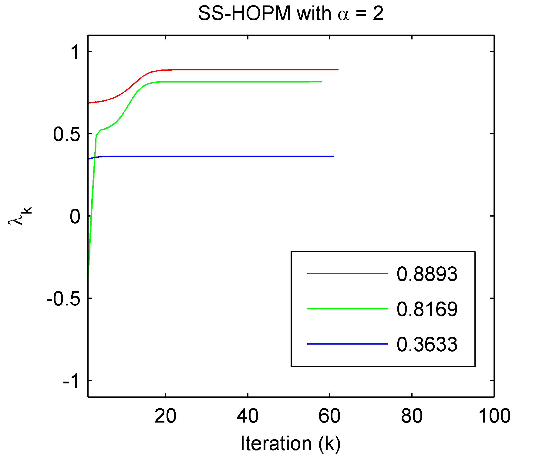
Again consider 𝓐[4,3]𝓐superscript43\bm{\mathscr{{A}}}\in\mathbb{R}^{[4,3]} from Example 3.23. We show results using a shift of α=2𝛼2\alpha=2. We ran 100 trials of SS-HOPM using the experimental conditions described in Example 3.23. We found 3 real eigenpairs; the results are summarized in Table 4a. Three example runs (one for each eigenvalue) are shown in Figure 2a.

We also considered the “conservative” choice of α=(m1)i1,,im|ai1im|=55.6620𝛼𝑚1subscriptsubscript𝑖1subscript𝑖𝑚subscript𝑎subscript𝑖1subscript𝑖𝑚55.6620\alpha=(m-1)\sum_{i_{1},\dots,i_{m}}|{a}_{i_{1}\dots i_{m}}|=55.6620. We ran 100 trials of SS-HOPM using the experimental conditions described in Example 3.23, except that we increased the maximum number of iterations to 10,000. Every trial converged to one of the same 3 real eigenpairs, but the number of iterations was around 1000 (versus around 60 for α=2𝛼2\alpha=2); in §4.2, we see that the rate of convergence asymptotically decreases as α𝛼\alpha increases.

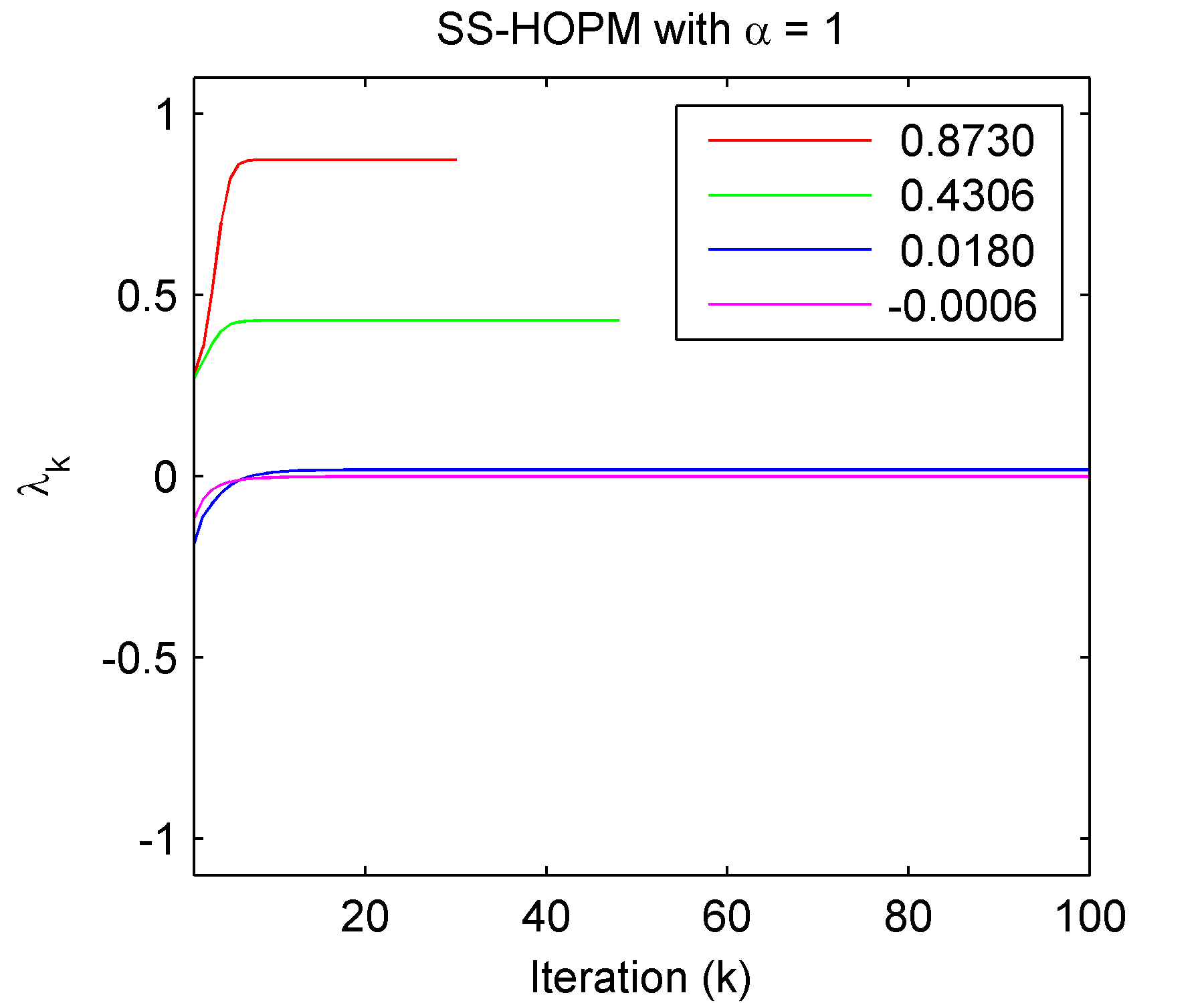
Analogous results are shown for 𝓐[3,3]𝓐superscript33\bm{\mathscr{{A}}}\in\mathbb{R}^{[3,3]} from Example 3.24 with a shift of α=1𝛼1\alpha=1 in Table 4b and Figure 2b. Here SS-HOPM finds 2 additional eigenpairs compared to S-HOPM. In this case, we also considered α=(m1)i1,,im|ai1im|=9.3560𝛼𝑚1subscriptsubscript𝑖1subscript𝑖𝑚subscript𝑎subscript𝑖1subscript𝑖𝑚9.3560\alpha=(m-1)\sum_{i_{1},\dots,i_{m}}|{a}_{i_{1}\dots i_{m}}|=9.3560, but this again increased the number of iterations up to a factor of ten.

For both tensors, {λk}subscript𝜆𝑘\{\lambda_{k}\} is always a nondecreasing sequence. Observe further that SS-HOPM converges only to eigenpairs that are negative stable.

# Occurrences λ𝜆\lambda 𝐱𝐱{\bm{\mathbf{{x}}}} Median Its.
46 0.88930.8893\phantom{-}0.8893 [ 0.66720.6672\phantom{-}0.6672 0.24710.2471\phantom{-}0.2471 0.70270.7027-0.7027 ] 63
24 0.81690.8169\phantom{-}0.8169 [ 0.84120.8412\phantom{-}0.8412 0.26350.2635-0.2635 0.47220.4722\phantom{-}0.4722 ] 52
30 0.36330.3633\phantom{-}0.3633 [ 0.26760.2676\phantom{-}0.2676 0.64470.6447\phantom{-}0.6447 0.71600.7160\phantom{-}0.7160 ] 65
(a) 𝓐[4,3]𝓐superscript43\bm{\mathscr{{A}}}\in\mathbb{R}^{[4,3]} from Example 3.23 with α=2𝛼2\alpha=2.
# Occurrences λ𝜆\lambda 𝐱𝐱{\bm{\mathbf{{x}}}} Median Its.
40 0.87300.8730\phantom{-}0.8730 [ 0.39220.3922-0.3922 0.72490.7249\phantom{-}0.7249 0.56640.5664\phantom{-}0.5664 ] 32
29 0.43060.4306\phantom{-}0.4306 [ 0.71870.7187-0.7187 0.12450.1245-0.1245 0.68400.6840-0.6840 ] 48
18 0.01800.0180\phantom{-}0.0180 [ 0.71320.7132\phantom{-}0.7132 0.50930.5093\phantom{-}0.5093 0.48170.4817-0.4817 ] 116
13 0.00060.0006-0.0006 [ 0.29070.2907-0.2907 0.73590.7359-0.7359 0.61150.6115\phantom{-}0.6115 ] 145
(b) 𝓐[3,3]𝓐superscript33\bm{\mathscr{{A}}}\in\mathbb{R}^{[3,3]} from Example 3.24 with α=1𝛼1\alpha=1.
Table 4: Eigenpairs computed by SS-HOPM (convex) with 100 random starts.
Refer to caption
(a) 𝓐[4,3]𝓐superscript43\bm{\mathscr{{A}}}\in\mathbb{R}^{[4,3]} from Example 3.23 with α=2𝛼2\alpha=2.
Refer to caption
(b) 𝓐[3,3]𝓐superscript33\bm{\mathscr{{A}}}\in\mathbb{R}^{[3,3]} from Example 3.24 with α=1𝛼1\alpha=1.
Fig. 2: Example λksubscript𝜆𝑘\lambda_{k} values for SS-HOPM (convex). One sequence is shown for each distinct eigenvalue.

Using a large enough negative value of α𝛼\alpha makes f^^𝑓\hat{f} concave. It was observed [11] that f(𝐱)=f(𝐱)𝑓𝐱𝑓𝐱f({\bm{\mathbf{{x}}}})=f(-{\bm{\mathbf{{x}}}}) for even-order tensors and so the sequence {λk}subscript𝜆𝑘\{\lambda_{k}\} converges regardless of correctly handling the minus sign. The only minor problem in the concave case is that the sequence of iterates {𝐱k}subscript𝐱𝑘\{{\bm{\mathbf{{x}}}}_{k}\} does not converge. This is easily fixed, however, by correctly handling the sign as we do in Algorithm 2. The corresponding theory for the concave case is presented in Corollary 4.34. In this case we choose α𝛼\alpha to be negative, i.e., the theory suggests α<β(𝓐)𝛼𝛽𝓐\alpha<-\beta(\bm{\mathscr{{A}}}).

Corollary 4.34.

Let 𝓐[m,n]𝓐superscript𝑚𝑛\bm{\mathscr{{A}}}\in\mathbb{R}^{[m,n]} be symmetric. For α<β(𝓐)𝛼𝛽𝓐\alpha<-\beta(\bm{\mathscr{{A}}}), where β(𝓐)𝛽𝓐\beta(\bm{\mathscr{{A}}}) is defined in (12), the iterates {λk,𝐱k}subscript𝜆𝑘subscript𝐱𝑘\{\lambda_{k},{\bm{\mathbf{{x}}}}_{k}\} produced by Algorithm 2 satisfy the following properties. (a) The sequence {λk}subscript𝜆𝑘\{\lambda_{k}\} is nonincreasing, and there exists λsubscript𝜆\lambda_{*} such that λkλsubscript𝜆𝑘subscript𝜆\lambda_{k}\rightarrow\lambda_{*}. (b) The sequence {𝐱k}subscript𝐱𝑘\{{\bm{\mathbf{{x}}}}_{k}\} has an accumulation point. (c) For any such accumulation point 𝐱subscript𝐱{\bm{\mathbf{{x}}}}_{*}, the pair (λ,𝐱)subscript𝜆subscript𝐱(\lambda_{*},{\bm{\mathbf{{x}}}}_{*}) is an eigenpair of 𝓐𝓐\bm{\mathscr{{A}}}. (d) If the eigenvalues of 𝓐𝓐\bm{\mathscr{{A}}} are isolated, then 𝐱k𝐱subscript𝐱𝑘subscript𝐱{\bm{\mathbf{{x}}}}_{k}\to{\bm{\mathbf{{x}}}}_{*}.

Proof 4.35.

Apply the proof of Theorem 4.31 with f(𝐱)=𝓐𝐱m𝑓𝐱𝓐superscript𝐱𝑚f({\bm{\mathbf{{x}}}})=-\bm{\mathscr{{A}}}{\bm{\mathbf{{x}}}}^{m}.

Example 4.36.

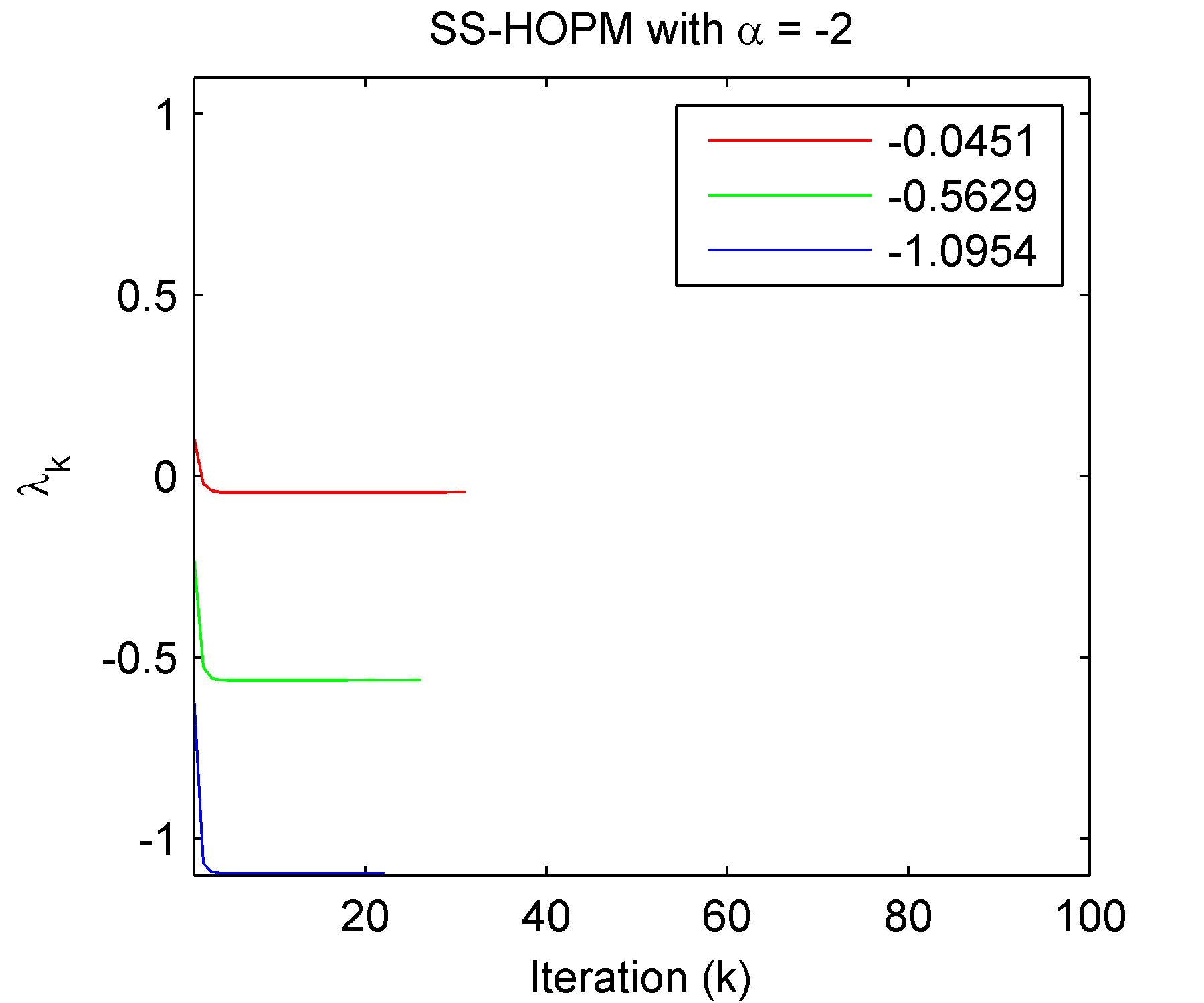
Revisiting 𝓐[4,3]𝓐superscript43\bm{\mathscr{{A}}}\in\mathbb{R}^{[4,3]} in Example 3.23 again, we run another 100 trials using α=2𝛼2\alpha=-2. We find 3 (new) real eigenpairs; the results are summarized in Table 5a. Three example runs (one for each eigenvalue) are shown in Figure 3a.

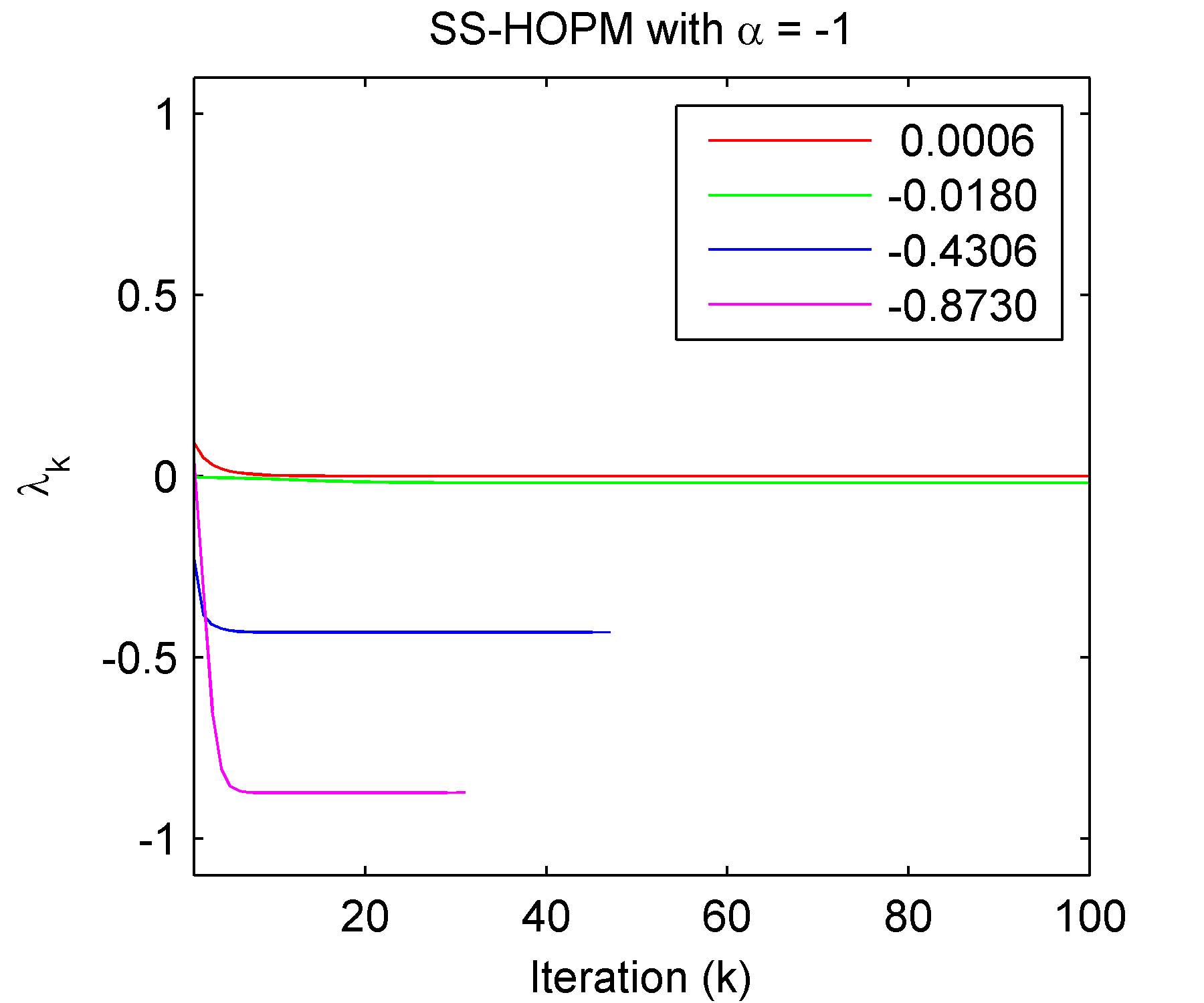
We also revisit 𝓐[3,3]𝓐superscript33\bm{\mathscr{{A}}}\in\mathbb{R}^{[3,3]} from Example 3.24 and use α=1𝛼1\alpha=-1. In this case, we find the opposites, i.e., (λ,𝐱)𝜆𝐱(-\lambda,-{\bm{\mathbf{{x}}}}), of the eigenpairs found with α=1𝛼1\alpha=1, as shown in Table 5b. This is to be expected for odd-order tensors since there is symmetry, i.e., f(𝐱)=f(𝐱)𝑓𝐱𝑓𝐱f({\bm{\mathbf{{x}}}})=-f(-{\bm{\mathbf{{x}}}}), C(λ,𝐱)=C(λ,𝐱)𝐶𝜆𝐱𝐶𝜆𝐱C(\lambda,{\bm{\mathbf{{x}}}})=-C(-\lambda,-{\bm{\mathbf{{x}}}}), etc. Observe that the median number of iterations is nearly unchanged; this is explained in the subsequent subsection where we discuss the rate of convergence. Four example runs (one per eigenvalue) are shown in Figure 3b.

The sequence {λk}subscript𝜆𝑘\{\lambda_{k}\} is nonincreasing in every case. Each of the eigenpairs found in the concave case is positive stable.

# Occurrences λ𝜆\lambda 𝐱𝐱{\bm{\mathbf{{x}}}} Median Its.
15 0.04510.0451-0.0451 [ 0.77970.7797-0.7797 0.61350.6135-0.6135 0.12500.1250-0.1250 ] 35
40 0.56290.5629-0.5629 [ 0.17620.1762-0.1762 0.17960.1796\phantom{-}0.1796 0.96780.9678-0.9678 ] 23
45 1.09541.0954-1.0954 [ 0.59150.5915-0.5915 0.74670.7467\phantom{-}0.7467 0.30430.3043\phantom{-}0.3043 ] 23
(a) 𝓐[4,3]𝓐superscript43\bm{\mathscr{{A}}}\in\mathbb{R}^{[4,3]} from Example 3.23 with α=2𝛼2\alpha=-2.
# Occurrences λ𝜆\lambda 𝐱𝐱{\bm{\mathbf{{x}}}} Median Its.
19 0.00060.0006\phantom{-}0.0006 [ 0.29070.2907\phantom{-}0.2907 0.73590.7359\phantom{-}0.7359 0.61150.6115-0.6115 ] 146
18 0.01800.0180-0.0180 [ 0.71320.7132-0.7132 0.50930.5093-0.5093 0.48170.4817\phantom{-}0.4817 ] 117
29 0.43060.4306-0.4306 [ 0.71870.7187\phantom{-}0.7187 0.12450.1245\phantom{-}0.1245 0.68400.6840\phantom{-}0.6840 ] 49
34 0.87300.8730-0.8730 [ 0.39220.3922\phantom{-}0.3922 0.72490.7249-0.7249 0.56640.5664-0.5664 ] 33
(b) 𝓐[3,3]𝓐superscript33\bm{\mathscr{{A}}}\in\mathbb{R}^{[3,3]} from Example 3.24 with α=1𝛼1\alpha=-1.
Table 5: Eigenpairs computed by SS-HOPM (concave) with 100 random starts.
Refer to caption
(a) 𝓐[4,3]𝓐superscript43\bm{\mathscr{{A}}}\in\mathbb{R}^{[4,3]} from Example 3.23 with α=2𝛼2\alpha=2.
Refer to caption
(b) 𝓐[3,3]𝓐superscript33\bm{\mathscr{{A}}}\in\mathbb{R}^{[3,3]} from Example 3.24 with α=1𝛼1\alpha=1.
Fig. 3: Example λksubscript𝜆𝑘\lambda_{k} values for SS-HOPM (concave). One sequence is shown for each distinct eigenvalue.

4.2 SS-HOPM fixed point analysis

In this section, we show that fixed point analysis allows us to easily characterize convergence to eigenpairs according to whether they are positive stable, negative stable, or unstable. The convex version of SS-HOPM will generically converge to eigenpairs that are negative stable; the concave version will generically converge to eigenpairs that are positive stable.

To justify these conclusions, we consider Algorithm 2 in the convex case as a fixed point iteration 𝐱k+1=ϕ(𝐱k;α)subscript𝐱𝑘1italic-ϕsubscript𝐱𝑘𝛼{\bm{\mathbf{{x}}}}_{k+1}=\phi({\bm{\mathbf{{x}}}}_{k};\alpha), where ϕitalic-ϕ\phi is defined as

ϕ(𝐱;α)=ϕ1(ϕ2(𝐱;α)) with ϕ1(𝐱)=𝐱(𝐱T𝐱)12 and ϕ2(𝐱;α)=𝓐𝐱m1+α𝐱.italic-ϕ𝐱𝛼subscriptitalic-ϕ1subscriptitalic-ϕ2𝐱𝛼 with subscriptitalic-ϕ1𝐱𝐱superscriptsuperscript𝐱𝑇𝐱12 and subscriptitalic-ϕ2𝐱𝛼𝓐superscript𝐱𝑚1𝛼𝐱\phi({\bm{\mathbf{{x}}}};\alpha)=\phi_{1}(\phi_{2}({\bm{\mathbf{{x}}}};\alpha))\text{ with }\phi_{1}({\bm{\mathbf{{x}}}})=\frac{{\bm{\mathbf{{x}}}}}{({\bm{\mathbf{{x}}}}^{T}{\bm{\mathbf{{x}}}})^{\frac{1}{2}}}\text{ and }\phi_{2}({\bm{\mathbf{{x}}}};\alpha)=\bm{\mathscr{{A}}}{\bm{\mathbf{{x}}}}^{m-1}+\alpha{\bm{\mathbf{{x}}}}. (19)

Note that an eigenpair (λ,𝐱)𝜆𝐱(\lambda,{\bm{\mathbf{{x}}}}) is a fixed point if and only if λ+α>0𝜆𝛼0\lambda+\alpha>0, which is always true for α>β(𝓐)𝛼𝛽𝓐\alpha>\beta(\bm{\mathscr{{A}}}).

From [9], the Jacobian of the operator ϕitalic-ϕ\phi is

J(𝐱;α)=ϕ1(ϕ2(𝐱;α))ϕ2(𝐱;α),𝐽𝐱𝛼superscriptsubscriptitalic-ϕ1subscriptitalic-ϕ2𝐱𝛼superscriptsubscriptitalic-ϕ2𝐱𝛼J({\bm{\mathbf{{x}}}};\alpha)=\phi_{1}^{\prime}(\phi_{2}({\bm{\mathbf{{x}}}};\alpha))\phi_{2}^{\prime}({\bm{\mathbf{{x}}}};\alpha),

where derivatives are taken with respect to 𝐱𝐱{\bm{\mathbf{{x}}}} and

ϕ1(𝐱)=(𝐱T𝐱)𝐈𝐱𝐱T(𝐱T𝐱)32andϕ2(𝐱;α)=(m1)𝓐𝐱m2+α𝐈.formulae-sequencesuperscriptsubscriptitalic-ϕ1𝐱superscript𝐱𝑇𝐱𝐈superscript𝐱𝐱𝑇superscriptsuperscript𝐱𝑇𝐱32andsuperscriptsubscriptitalic-ϕ2𝐱𝛼𝑚1𝓐superscript𝐱𝑚2𝛼𝐈\phi_{1}^{\prime}({\bm{\mathbf{{x}}}})=\frac{({\bm{\mathbf{{x}}}}^{T}{\bm{\mathbf{{x}}}}){\bm{\mathbf{{I}}}}-{\bm{\mathbf{{x}}}}{\bm{\mathbf{{x}}}}^{T}}{({\bm{\mathbf{{x}}}}^{T}{\bm{\mathbf{{x}}}})^{\frac{3}{2}}}\quad\text{and}\quad\phi_{2}^{\prime}({\bm{\mathbf{{x}}}};\alpha)=(m-1)\bm{\mathscr{{A}}}{\bm{\mathbf{{x}}}}^{m-2}+\alpha{\bm{\mathbf{{I}}}}.

At any eigenpair (λ,𝐱)𝜆𝐱(\lambda,{\bm{\mathbf{{x}}}}), we have

ϕ2(𝐱;α)=(λ+α)𝐱,ϕ1(ϕ2(𝐱;α))=(𝐈𝐱𝐱T)λ+α,formulae-sequencesubscriptitalic-ϕ2𝐱𝛼𝜆𝛼𝐱superscriptsubscriptitalic-ϕ1subscriptitalic-ϕ2𝐱𝛼𝐈superscript𝐱𝐱𝑇𝜆𝛼\displaystyle\phi_{2}({\bm{\mathbf{{x}}}};\alpha)=(\lambda+\alpha){\bm{\mathbf{{x}}}},\quad\phi_{1}^{\prime}(\phi_{2}({\bm{\mathbf{{x}}}};\alpha))=\frac{({\bm{\mathbf{{I}}}}-{\bm{\mathbf{{x}}}}{\bm{\mathbf{{x}}}}^{T})}{\lambda+\alpha},
andϕ2(𝐱;α)=(m1)𝓐𝐱m2+α𝐈.andsuperscriptsubscriptitalic-ϕ2𝐱𝛼𝑚1𝓐superscript𝐱𝑚2𝛼𝐈\displaystyle\quad\text{and}\quad\phi_{2}^{\prime}({\bm{\mathbf{{x}}}};\alpha)=(m-1)\bm{\mathscr{{A}}}{\bm{\mathbf{{x}}}}^{m-2}+\alpha{\bm{\mathbf{{I}}}}.

Thus, the Jacobian at 𝐱𝐱{\bm{\mathbf{{x}}}} is

J(𝐱;α)=(m1)(𝓐𝐱m2λ𝐱𝐱T)+α(𝐈𝐱𝐱T)λ+α.𝐽𝐱𝛼𝑚1𝓐superscript𝐱𝑚2𝜆superscript𝐱𝐱𝑇𝛼𝐈superscript𝐱𝐱𝑇𝜆𝛼J({\bm{\mathbf{{x}}}};\alpha)=\frac{(m-1)(\bm{\mathscr{{A}}}{\bm{\mathbf{{x}}}}^{m-2}-\lambda{\bm{\mathbf{{x}}}}{\bm{\mathbf{{x}}}}^{T})+\alpha({\bm{\mathbf{{I}}}}-{\bm{\mathbf{{x}}}}{\bm{\mathbf{{x}}}}^{T})}{\lambda+\alpha}. (20)

Observe that the Jacobian is symmetric.

Theorem 4.37.

Let (λ,𝐱)𝜆𝐱(\lambda,{\bm{\mathbf{{x}}}}) be an eigenpair of a symmetric tensor 𝓐[m,n]𝓐superscript𝑚𝑛\bm{\mathscr{{A}}}\in\mathbb{R}^{[m,n]}. Assume α𝛼\alpha\in\mathbb{R} such that α>β(𝓐)𝛼𝛽𝓐\alpha>\beta(\bm{\mathscr{{A}}}), where β(𝓐)𝛽𝓐\beta(\bm{\mathscr{{A}}}) is as defined in (12). Let ϕ(𝐱)italic-ϕ𝐱\phi({\bm{\mathbf{{x}}}}) be given by (19). Then (λ,𝐱)𝜆𝐱(\lambda,{\bm{\mathbf{{x}}}}) is negative stable if and only if 𝐱𝐱{\bm{\mathbf{{x}}}} is a linearly attracting fixed point of ϕitalic-ϕ\phi.

Proof 4.38.

Assume that (λ,𝐱)𝜆𝐱(\lambda,{\bm{\mathbf{{x}}}}) is negative stable. The Jacobian J(𝐱;α)𝐽𝐱𝛼J({\bm{\mathbf{{x}}}};\alpha) is given by (20). By Theorem 2.14, we need to show that ρ(J(𝐱;α))<1𝜌𝐽𝐱𝛼1\rho(J({\bm{\mathbf{{x}}}};\alpha))<1 or, equivalently since J(𝐱;α)𝐽𝐱𝛼J({\bm{\mathbf{{x}}}};\alpha) is symmetric, |𝐲TJ(𝐱;α)𝐲|<1superscript𝐲𝑇𝐽𝐱𝛼𝐲1|{\bm{\mathbf{{y}}}}^{T}J({\bm{\mathbf{{x}}}};\alpha){\bm{\mathbf{{y}}}}|<1 for all 𝐲Σ𝐲Σ{\bm{\mathbf{{y}}}}\in\Sigma. We restrict our attention to 𝐲𝐱bottom𝐲𝐱{\bm{\mathbf{{y}}}}\bot{\bm{\mathbf{{x}}}} since J(𝐱;α)𝐱=𝟎𝐽𝐱𝛼𝐱0J({\bm{\mathbf{{x}}}};\alpha){\bm{\mathbf{{x}}}}={\bm{\mathbf{{0}}}}.

Let 𝐲Σ𝐲Σ{\bm{\mathbf{{y}}}}\in\Sigma with 𝐲𝐱bottom𝐲𝐱{\bm{\mathbf{{y}}}}\bot{\bm{\mathbf{{x}}}}. Then

|𝐲TJ(𝐱;α)𝐲|=|𝐲T((m1)𝓐𝐱m2)𝐲+αλ+α|superscript𝐲𝑇𝐽𝐱𝛼𝐲superscript𝐲𝑇𝑚1𝓐superscript𝐱𝑚2𝐲𝛼𝜆𝛼|{\bm{\mathbf{{y}}}}^{T}J({\bm{\mathbf{{x}}}};\alpha){\bm{\mathbf{{y}}}}|=\left|\frac{{\bm{\mathbf{{y}}}}^{T}\left((m-1)\bm{\mathscr{{A}}}{\bm{\mathbf{{x}}}}^{m-2}\right){\bm{\mathbf{{y}}}}+\alpha}{\lambda+\alpha}\right|

The assumption that (λ,𝐱)𝜆𝐱(\lambda,{\bm{\mathbf{{x}}}}) is negative stable means that C(λ,𝐱)𝐶𝜆𝐱C(\lambda,{\bm{\mathbf{{x}}}}) is negative definite; therefore, 𝐲T((m1)𝓐𝐱m2)𝐲<λ.superscript𝐲𝑇𝑚1𝓐superscript𝐱𝑚2𝐲𝜆{\bm{\mathbf{{y}}}}^{T}\left((m-1)\bm{\mathscr{{A}}}{\bm{\mathbf{{x}}}}^{m-2}\right){\bm{\mathbf{{y}}}}<\lambda. On the other hand, by the definition of β𝛽\beta,

ρ((m1)𝓐𝐱m2)β(𝓐).𝜌𝑚1𝓐superscript𝐱𝑚2𝛽𝓐\rho\!\left((m-1)\bm{\mathscr{{A}}}{\bm{\mathbf{{x}}}}^{m-2}\right)\leq\beta(\bm{\mathscr{{A}}}).

Thus, using the fact that λ+α𝜆𝛼\lambda+\alpha is positive, we have

0<β(𝓐)+αλ+α𝐲T((m1)𝓐𝐱m2)𝐲+αλ+α<λ+αλ+α=10𝛽𝓐𝛼𝜆𝛼superscript𝐲𝑇𝑚1𝓐superscript𝐱𝑚2𝐲𝛼𝜆𝛼𝜆𝛼𝜆𝛼10<\frac{-\beta(\bm{\mathscr{{A}}})+\alpha}{\lambda+\alpha}\leq\frac{{\bm{\mathbf{{y}}}}^{T}\left((m-1)\bm{\mathscr{{A}}}{\bm{\mathbf{{x}}}}^{m-2}\right){\bm{\mathbf{{y}}}}+\alpha}{\lambda+\alpha}<\frac{\lambda+\alpha}{\lambda+\alpha}=1

Hence, ρ(J(𝐱;α))<1𝜌𝐽𝐱𝛼1\rho(J({\bm{\mathbf{{x}}}};\alpha))<1, and 𝐱𝐱{\bm{\mathbf{{x}}}} is a linearly attracting fixed point.

On the other hand, if (λ,𝐱)𝜆𝐱(\lambda,{\bm{\mathbf{{x}}}}) is not negative stable, then there exists 𝐰Σ𝐰Σ{\bm{\mathbf{{w}}}}\in\Sigma such that 𝐰𝐱bottom𝐰𝐱{\bm{\mathbf{{w}}}}\bot{\bm{\mathbf{{x}}}} and 𝐰T((m1)𝓐𝐱m2)𝐰λsuperscript𝐰𝑇𝑚1𝓐superscript𝐱𝑚2𝐰𝜆{\bm{\mathbf{{w}}}}^{T}\left((m-1)\bm{\mathscr{{A}}}{\bm{\mathbf{{x}}}}^{m-2}\right){\bm{\mathbf{{w}}}}\geq\lambda. Thus,

𝐰TJ(𝐱;α)𝐰=𝐰T((m1)𝓐𝐱m2)𝐰+αλ+αλ+αλ+α=1.superscript𝐰𝑇𝐽𝐱𝛼𝐰superscript𝐰𝑇𝑚1𝓐superscript𝐱𝑚2𝐰𝛼𝜆𝛼𝜆𝛼𝜆𝛼1{\bm{\mathbf{{w}}}}^{T}J({\bm{\mathbf{{x}}}};\alpha){\bm{\mathbf{{w}}}}=\frac{{\bm{\mathbf{{w}}}}^{T}\left((m-1)\bm{\mathscr{{A}}}{\bm{\mathbf{{x}}}}^{m-2}\right){\bm{\mathbf{{w}}}}+\alpha}{\lambda+\alpha}\geq\frac{\lambda+\alpha}{\lambda+\alpha}=1.

Consequently, ρ(J(𝐱;α))1𝜌𝐽𝐱𝛼1\rho(J({\bm{\mathbf{{x}}}};\alpha))\geq 1, and 𝐱𝐱{\bm{\mathbf{{x}}}} is not a linearly attracting fixed point by Theorem 2.14 and Theorem 2.15.

In fact, we can see from the proof of Theorem 4.37 that if the eigenpair (λ,𝐱)𝜆𝐱(\lambda,{\bm{\mathbf{{x}}}}) is not negative stable, there is no choice of α𝛼\alpha\in\mathbb{R} that will make ρ(J(𝐱;α))<1𝜌𝐽𝐱𝛼1\rho(J({\bm{\mathbf{{x}}}};\alpha))<1. For 𝐱𝐱{\bm{\mathbf{{x}}}} to be a fixed point at all, we must have λ+α>0𝜆𝛼0\lambda+\alpha>0, and this is sufficient to obtain ρ(J(𝐱;α))1𝜌𝐽𝐱𝛼1\rho(J({\bm{\mathbf{{x}}}};\alpha))\geq 1 if (λ,𝐱)𝜆𝐱(\lambda,{\bm{\mathbf{{x}}}}) is not negative stable. In other words, smaller values of α𝛼\alpha do not induce “accidental” convergence to any additional eigenpairs.

An alternative argument establishes, for α>β(𝓐)𝛼𝛽𝓐\alpha>\beta(\bm{\mathscr{{A}}}), the slightly broader result that any attracting fixed point, regardless of order of convergence, must be a strict constrained local maximum of f(𝐱)=𝓐𝐱m𝑓𝐱𝓐superscript𝐱𝑚f({\bm{\mathbf{{x}}}})=\bm{\mathscr{{A}}}{\bm{\mathbf{{x}}}}^{m} on ΣΣ\Sigma. That is, the marginally attracting case corresponds to a stationary point that has degenerate C(λ,𝐱)𝐶𝜆𝐱C(\lambda,{\bm{\mathbf{{x}}}}) but is still a maximum. This follows from Theorem 2.9, where the needed convexity holds for α>β(𝓐)𝛼𝛽𝓐\alpha>\beta(\bm{\mathscr{{A}}}), so that any vector 𝐱Σsuperscript𝐱Σ{\bm{\mathbf{{x}}}}^{\prime}\in\Sigma in the neighborhood of convergence of 𝐱𝐱{\bm{\mathbf{{x}}}} must satisfy f(𝐱)<f(𝐱)𝑓superscript𝐱𝑓𝐱f({\bm{\mathbf{{x}}}}^{\prime})<f({\bm{\mathbf{{x}}}}). One can convince oneself that the converse also holds for α>β(𝓐)𝛼𝛽𝓐\alpha>\beta(\bm{\mathscr{{A}}}), i.e., any strict local maximum corresponds to an attracting fixed point. This is because the strict monotonicity of f𝑓f under iteration (other than at a fixed point) implies that the iteration acts as a contraction on the region of closed contours of f𝑓f around the maximum.

The counterpart of Theorem 4.37 for the concave case is as follows.

Corollary 4.39.

Let (λ,𝐱)𝜆𝐱(\lambda,{\bm{\mathbf{{x}}}}) be an eigenpair of a symmetric tensor 𝓐[m,n]𝓐superscript𝑚𝑛\bm{\mathscr{{A}}}\in\mathbb{R}^{[m,n]}. Assume α𝛼\alpha\in\mathbb{R} such that α<β(𝓐)𝛼𝛽𝓐\alpha<-\beta(\bm{\mathscr{{A}}}), where β(𝓐)𝛽𝓐\beta(\bm{\mathscr{{A}}}) is as defined in (12). Let ϕ(𝐱)italic-ϕ𝐱\phi({\bm{\mathbf{{x}}}}) be given by (19). Then (λ,𝐱)𝜆𝐱(\lambda,{\bm{\mathbf{{x}}}}) is positive stable if and only if 𝐱𝐱{\bm{\mathbf{{x}}}} is a linearly attracting fixed point of ϕitalic-ϕ-\phi.

Example 4.40.

We return again to 𝓐[4,3]𝓐superscript43\bm{\mathscr{{A}}}\in\mathbb{R}^{[4,3]} as defined in Example 3.23. Figure 4a shows the spectral radius of the Jacobian of the fixed point iteration for varying values of α𝛼\alpha for all eigenpairs that are positive or negative stable. At α=0𝛼0\alpha=0, the spectral radius is greater than 1 for every eigenvalue, and this is why S-HOPM never converges. At α=2𝛼2\alpha=2, on the other hand, we see that the spectral radius is less than 1 for all of the negative stable eigenpairs. Furthermore, the spectral radius stays less than 1 as α𝛼\alpha increases. Conversely, at α=2𝛼2\alpha=-2, the spectral radius is less than 1 for all the eigenpairs that are positive stable.

In Figure 5a, we plot example iteration sequences for 𝐱k+1𝐱/𝐱k𝐱normsubscript𝐱𝑘1subscript𝐱normsubscript𝐱𝑘subscript𝐱\|{\bm{\mathbf{{x}}}}_{k+1}-{\bm{\mathbf{{x}}}}_{*}\|/\|{\bm{\mathbf{{x}}}}_{k}-{\bm{\mathbf{{x}}}}_{*}\| for each eigenpair, using α=2𝛼2\alpha=2 for the negative stable eigenpairs and α=2𝛼2\alpha=-2 for the positive stable eigenpairs. We expect 𝐱k+1𝐱=σ𝐱k𝐱normsubscript𝐱𝑘1subscript𝐱𝜎normsubscript𝐱𝑘subscript𝐱\|{\bm{\mathbf{{x}}}}_{k+1}-{\bm{\mathbf{{x}}}}_{*}\|=\sigma\|{\bm{\mathbf{{x}}}}_{k}-{\bm{\mathbf{{x}}}}_{*}\| where σ𝜎\sigma is the spectral radius of the Jacobian J(𝐱;α)𝐽𝐱𝛼J({\bm{\mathbf{{x}}}};\alpha). For example, for λ=1.0954𝜆1.0954\lambda=-1.0954, we have σ=0.4𝜎0.4\sigma=0.4 (shown as a dashed line) and this precisely matched the observed rate of convergence (shown as a solid line).

Figure 6a plots f(𝐱)𝑓𝐱f({\bm{\mathbf{{x}}}}) on the unit sphere using color to indicate function value. We show the front and back of the sphere. Notice that the horizontal axis is from 111 to 11-1 in the left plot and from 11-1 to 111 in the right plot, as if walking around the sphere. In this image, the horizontal axis corresponds to x2subscript𝑥2x_{2} and the vertical axis to x3subscript𝑥3x_{3}; the left image is centered at x1=1subscript𝑥11x_{1}=1 and the right image at x1=1subscript𝑥11x_{1}=-1. Since m𝑚m is even, the function is symmetric, i.e., f(𝐱)=f(𝐱)𝑓𝐱𝑓𝐱f({\bm{\mathbf{{x}}}})=f(-{\bm{\mathbf{{x}}}}). The eigenvectors are shown as white, gray, and black circles corresponding to their classification as negative stable, positive stable, and unstable, respectively; in turn, these correspond to maxima, minima, and saddle points of f(𝐱)𝑓𝐱f({\bm{\mathbf{{x}}}}).

Figure 6b shows the basins of attraction for SS-HOPM with α=2𝛼2\alpha=2. Every grid point on the sphere was used as a starting point for SS-HOPM, and it is colored444Specifically, each block on the sphere is colored according to the convergence of its lower left point. according to which eigenvalue it converged to. In this case, every run converges to a negative stable eigenpair (labeled with a white circle). Recall that SS-HOPM must converge to some eigenpair per Theorem 4.31, and Theorem 4.37 says that it is generically a negative stable eigenpair. Thus, the non-attracting points lie on the boundaries of the domains of attraction.

Figure 6c shows the basins of attraction for SS-HOPM with α=2𝛼2\alpha=-2. In this case, every starting point converges to an eigenpair that is positive stable (shown as gray circles).
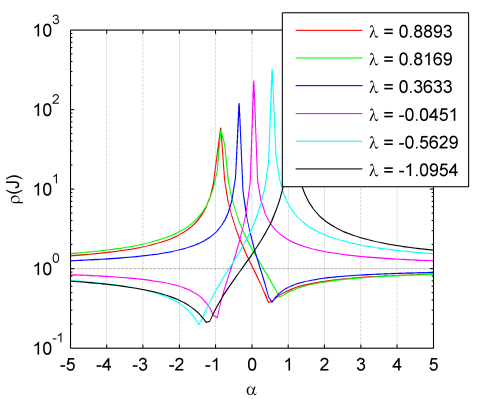
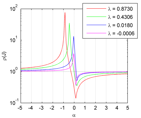
Refer to caption
(a) 𝓐[4,3]𝓐superscript43\bm{\mathscr{{A}}}\in\mathbb{R}^{[4,3]} from Example 3.23.
Refer to caption
(b) 𝓐[3,3]𝓐superscript33\bm{\mathscr{{A}}}\in\mathbb{R}^{[3,3]} from Example 3.24.
Fig. 4: Spectral radii of the Jacobian J(𝐱;α)𝐽𝐱𝛼J({\bm{\mathbf{{x}}}};\alpha) for different eigenpairs as α𝛼\alpha varies.
Refer to caption
(a) 𝓐[4,3]𝓐superscript43\bm{\mathscr{{A}}}\in\mathbb{R}^{[4,3]} from Example 3.23 using α=±2𝛼plus-or-minus2\alpha=\pm 2, as appropriate.
Refer to caption
(b) 𝓐[3,3]𝓐superscript33\bm{\mathscr{{A}}}\in\mathbb{R}^{[3,3]} from Example 3.24 using α=1𝛼1\alpha=1.
Fig. 5: Example plots of 𝐱k+1𝐱/𝐱k𝐱normsubscript𝐱𝑘1subscript𝐱normsubscript𝐱𝑘subscript𝐱\|{\bm{\mathbf{{x}}}}_{k+1}-{\bm{\mathbf{{x}}}}_{*}\|/\|{\bm{\mathbf{{x}}}}_{k}-{\bm{\mathbf{{x}}}}_{*}\|. The expected rate of convergence from J(𝐱;α)𝐽subscript𝐱𝛼J({\bm{\mathbf{{x}}}}_{*};\alpha) is shown as a dashed line.
Refer to caption
(a) Function values for f(𝐱)=𝓐𝐱m𝑓𝐱𝓐superscript𝐱𝑚f({\bm{\mathbf{{x}}}})=\bm{\mathscr{{A}}}{\bm{\mathbf{{x}}}}^{m}.
Refer to caption
(b) SS-HOPM basins of attraction using α=2𝛼2\alpha=2.
Refer to caption
(c) SS-HOPM basins of attraction using α=2𝛼2\alpha=-2.
Fig. 6: Illustrations for 𝓐[4,3]𝓐superscript43\bm{\mathscr{{A}}}\in\mathbb{R}^{[4,3]} from Example 3.23. The horizontal axis corresponds to x2subscript𝑥2{x}_{2} and the vertical axis to x3subscript𝑥3{x}_{3}; the left image is centered at x1=1subscript𝑥11{x}_{1}=1 and the right at x1=1subscript𝑥11{x}_{1}=-1. White, gray, and black dots indicate eigenvectors that are negative stable, positive stable, and unstable, respectively.
Refer to caption
(a) Function values for f(𝐱)=𝓐𝐱m𝑓𝐱𝓐superscript𝐱𝑚f({\bm{\mathbf{{x}}}})=\bm{\mathscr{{A}}}{\bm{\mathbf{{x}}}}^{m}.
Refer to caption
(b) SS-HOPM basins of attraction using α=0𝛼0\alpha=0.
Refer to caption
(c) SS-HOPM basins of attraction using α=1𝛼1\alpha=1.
Fig. 7: Illustrations for 𝓐[3,3]𝓐superscript33\bm{\mathscr{{A}}}\in\mathbb{R}^{[3,3]} from Example 3.24. The horizontal axis corresponds to x2subscript𝑥2{x}_{2} and the vertical axis to x3subscript𝑥3{x}_{3}; the left image is centered at x1=1subscript𝑥11{x}_{1}=1 and the right at x1=1subscript𝑥11{x}_{1}=-1. White, gray, and black dots indicate eigenvectors that are negative stable, positive stable, and unstable, respectively.
Example 4.41.

We return again to 𝓐[3,3]𝓐superscript33\bm{\mathscr{{A}}}\in\mathbb{R}^{[3,3]} from Example 3.24, which is interesting because S-HOPM was able to find 2 of its eigenpairs without any shift. In Figure 7a, f(𝐱)𝑓𝐱f({\bm{\mathbf{{x}}}}) is plotted on the unit sphere, along with each eigenvector, colored white, gray, or black based on whether it is negative stable, positive stable, or unstable, respectively. Observe that the function is antisymmetric, i.e., f(𝐱)=f(𝐱)𝑓𝐱𝑓𝐱f({\bm{\mathbf{{x}}}})=-f(-{\bm{\mathbf{{x}}}}). Figure 7b shows the basins of attraction for S-HOPM (i.e., SS-HOPM with α=0𝛼0\alpha=0). Every starting point converges to one of the 2 labeled eigenpairs. This is not surprising because Figure 4b shows that there are 2 eigenvalues for which the spectral radius of the Jacobian is less than 1 (λ=0.8730𝜆0.8730\lambda=0.8730 and 0.43060.43060.4306). The other 2 eigenvalues are non-attracting for α=0𝛼0\alpha=0. Figure 5b shows the observed rates of convergence.

Figure 7c shows the basins of attraction for SS-HOPM with α=1𝛼1\alpha=1; each negative stable eigenpair (shown as a white circle) is an attracting eigenpair. The concave case is just a mirror image and is not shown.

As the previous example reminds us, for odd order, there is no need to try both positive and negative α𝛼\alpha because the definiteness of C𝐶C flips for eigenvectors of opposite sign.

Two additional examples of SS-HOPM are presented in Appendix A.

4.3 Relationship to power method for matrix eigenpairs

The power method for matrix eigenpairs is a technique for finding the largest-magnitude eigenvalue (and corresponding eigenvector) of a diagonalizable symmetric matrix [10]. Let 𝐀𝐀{\bm{\mathbf{{A}}}} be a symmetric real-valued n×n𝑛𝑛n\times n matrix. Then the matrix power method is defined by

𝐱k+1=𝐀𝐱k𝐀𝐱k.subscript𝐱𝑘1subscript𝐀𝐱𝑘normsubscript𝐀𝐱𝑘{\bm{\mathbf{{x}}}}_{k+1}=\frac{{\bm{\mathbf{{A}}}}{\bm{\mathbf{{x}}}}_{k}}{\|{\bm{\mathbf{{A}}}}{{\bm{\mathbf{{x}}}}_{k}}\|}.

Assume that 𝐕𝚲𝐕T𝐕𝚲superscript𝐕𝑇{\bm{\mathbf{{V}}}}{\bm{\mathbf{{\Lambda}}}}{\bm{\mathbf{{V}}}}^{T} is the Schur decomposition of 𝐀𝐀{\bm{\mathbf{{A}}}} with eigenvalues satisfying |λ1|>|λ2||λn|subscript𝜆1subscript𝜆2subscript𝜆𝑛|\lambda_{1}|>|\lambda_{2}|\geq\cdots\geq|\lambda_{n}| (note the strict difference in the first 2 eigenvalues). The sequence {𝐱k}subscript𝐱𝑘\{{\bm{\mathbf{{x}}}}_{k}\} produced by the matrix power method always converges (up to sign) to the eigenvector associated with λ1subscript𝜆1\lambda_{1}. Shifting the matrix by 𝐀𝐀+α𝐈𝐀𝐀𝛼𝐈{\bm{\mathbf{{A}}}}\leftarrow{\bm{\mathbf{{A}}}}+\alpha{\bm{\mathbf{{I}}}} shifts the eigenvalues by λjλj+αsubscript𝜆𝑗subscript𝜆𝑗𝛼\lambda_{j}\leftarrow\lambda_{j}+\alpha, potentially altering which eigenvalue has the largest magnitude.

In the matrix case, the eigenvalues of the Jacobian defined by (20) for an eigenpair (λj,𝐱j)subscript𝜆𝑗subscript𝐱𝑗(\lambda_{j},{\bm{\mathbf{{x}}}}_{j}) are given by

{0}{λi+αλj+α:1in with ij}.0conditional-setsubscript𝜆𝑖𝛼subscript𝜆𝑗𝛼1𝑖𝑛 with 𝑖𝑗\{0\}\cup\left\{\frac{\lambda_{i}+\alpha}{\lambda_{j}+\alpha}:1\leq i\leq n\text{ with }i\neq j\right\}.

Thus, the Jacobian at 𝐱1subscript𝐱1{\bm{\mathbf{{x}}}}_{1} is the only one such that ρ(J(𝐱;α))<1𝜌𝐽𝐱𝛼1\rho(J({\bm{\mathbf{{x}}}};\alpha))<1; no other eigenvectors are stable fixed points of the iteration. This corresponds to Theorem 4.37 (or Corollary 4.39), since the most positive eigenvalue is negative stable, the most negative eigenvalue is positive stable, and every other eigenvalue is unstable. The eigenpair (λ1,𝐱1)subscript𝜆1subscript𝐱1(\lambda_{1},{\bm{\mathbf{{x}}}}_{1}) is an attractor for ordinary (convex) power iteration if λ1>0subscript𝜆10\lambda_{1}>0 or for flipped (concave) power iteration if λ1<0subscript𝜆10\lambda_{1}<0.

In contrast to the matrix power method, SS-HOPM can find multiple eigenpairs since there may be multiple positive and negative stable eigenpairs. But, as for matrices, since the most positive and most negative eigenvalues correspond to the global maximum and minimum of f(𝐱)𝑓𝐱f({\bm{\mathbf{{x}}}}), they must be negative stable and positive stable respectively. Thus, choosing α𝛼\alpha positive is necessary for finding the most positive tensor eigenvalue; conversely, α𝛼\alpha negative is necessary for finding the most negative tensor eigenvalue. Unfortunately, the ability to find multiple eigenpairs means that there is no guarantee that the iterates will converge to an extremal eigenpair from every starting point. In fact, multiple starting points may be needed.

4.4 Comparison to other methods

SS-HOPM is useful for its guaranteed convergence properties and its simple implementation based on tensor-vector multiplication. For fixed m𝑚m and large n𝑛n, the computational complexity of each iteration of SS-HOPM is O(nm)𝑂superscript𝑛𝑚O(n^{m}), which is the number of individual terms to be computed in 𝓐𝐱m1𝓐superscript𝐱𝑚1\bm{\mathscr{{A}}}{\bm{\mathbf{{x}}}}^{m-1}. This is analogous to the O(n2)𝑂superscript𝑛2O(n^{2}) complexity of matrix-vector multiplication as used in the matrix power method. We do not yet know how the number of iterations needed for numerical convergence of SS-HOPM depends on m𝑚m and n𝑛n.

The convergence of SS-HOPM to only a subset of eigenvalues, which tend to be among the largest in magnitude, is beneficial when the large eigenvalues are of primary interest, as in the rank-1 approximation problem [11]. In particular, the most positive eigenvalue and most negative eigenvalue always have a region of stable convergence for a suitable choice of shift. However, the lack of stable convergence to certain other eigenvalues is a disadvantage if those eigenvalues are of interest.

One evident computational approach for finding tensor eigenpairs should be compared with SS-HOPM. This is to apply a numerical solver for nonlinear equation systems, such as Newton’s method, directly to the eigenvalue equations (2). The computational complexity of each iteration of Newton’s method for this system is that of SS-HOPM plus the construction and inversion of the (n+1)×(n+1)𝑛1𝑛1(n+1)\times(n+1) Jacobian for (λ,𝐱)𝜆𝐱(\lambda,{\bm{\mathbf{{x}}}}). The Jacobian construction is effectively included in SS-HOPM, since it is dominated by computing 𝓐𝐱m2𝓐superscript𝐱𝑚2\bm{\mathscr{{A}}}{\bm{\mathbf{{x}}}}^{m-2}, which is a precursor of 𝓐𝐱m1𝓐superscript𝐱𝑚1\bm{\mathscr{{A}}}{\bm{\mathbf{{x}}}}^{m-1}. The additional work for inversion is O(n3)𝑂superscript𝑛3O(n^{3}), and for m3𝑚3m\geq 3 it does not affect the complexity scaling, which remains O(nm)𝑂superscript𝑛𝑚O(n^{m}).

Two advantages of an approach such as Newton’s method are generic locally stable convergence, which enables finding eigenpairs not found by SS-HOPM, and the quadratic order of convergence, which can be expected to require fewer iterations than the linearly convergent SS-HOPM. On the other hand, there is no known guarantee of global convergence as there is for SS-HOPM, and it is possible that many starting points fail to converge. Even those that do converge may lead to eigenpairs of less interest for a particular application. Furthermore, certain tensor structures can be more efficiently handled with SS-HOPM than with Newton’s method. For example, consider a higher-order symmetric tensor expressed as a sum of terms, each of which is an outer product of matrices. The computation of 𝓐𝐱m1𝓐superscript𝐱𝑚1\bm{\mathscr{{A}}}{\bm{\mathbf{{x}}}}^{m-1} then reduces to a series of matrix-vector multiplications, which are O(n2)𝑂superscript𝑛2O(n^{2}). This compares favorably to the O(n3)𝑂superscript𝑛3O(n^{3}) of Newton’s method for the same tensor. Further investigation of general nonlinear solver approaches to the tensor eigenvalue problem will be beneficial.

Finally, we consider a polynomial solver approach, such as we implemented in Mathematica. This can find all eigenpairs (subject to numerical conditioning issues) but becomes computationally expensive for large m𝑚m and n𝑛n. In part this is simply because, from Theorem 5.44, the number of eigenpairs grows exponentially with n𝑛n. The solver in Mathematica is designed to find all solutions; it is not clear whether a substantial improvement in efficiency would be possible if only one or a few solutions were required.

Nevertheless, for comparison with the iterative approaches discussed above, we have measured the computational time per eigenpair on a desktop computer for various values of m𝑚m and n𝑛n, as shown in Figure 8. The complexity of the polynomial solution, even measured per eigenpair, is seen to increase extremely rapidly (faster than exponentially) with n𝑛n. Thus the polynomial solver approach is not expected to be practical for large n𝑛n.

Refer to caption
Fig. 8: Average time (over 10 trials) required to compute all eigenpairs, divided by the number of eigenpairs, for random symmetric tensors in [m,n]superscript𝑚𝑛\mathbb{R}^{[m,n]}. Note logarithmic vertical scale. Measured using NSolve in Mathematica on a 4 GHz Intel Core i7.

5 Complex case

We present the more general definition of complex eigenpairs and some related results, and propose an extension of the SS-HOPM algorithm to this case.

5.1 Eigenrings

Some of the solutions of the polynomial system that results from the eigenvalue equations may be complex; thus, the definition can be extended to the complex case as follows, where denotes the conjugate transpose.

Definition 5.42.

Assume that 𝓐𝓐\bm{\mathscr{{A}}} is a symmetric mthsuperscript𝑚thm^{\text{th}}-order n𝑛n-dimensional real-valued tensor. Then λ𝜆\lambda\in\mathbb{C} is an eigenvalue of 𝓐𝓐\bm{\mathscr{{A}}} if there exists 𝐱n𝐱superscript𝑛{\bm{\mathbf{{x}}}}\in\mathbb{C}^{n} such that

𝓐𝐱m1=λ𝐱and𝐱𝐱=1.formulae-sequence𝓐superscript𝐱𝑚1𝜆𝐱andsuperscript𝐱𝐱1\bm{\mathscr{{A}}}{\bm{\mathbf{{x}}}}^{m-1}=\lambda{\bm{\mathbf{{x}}}}\quad\text{and}\quad{\bm{\mathbf{{x}}}}^{\dagger}{\bm{\mathbf{{x}}}}=1. (21)

The vector 𝐱𝐱{\bm{\mathbf{{x}}}} is a corresponding eigenvector, and (λ,𝐱)𝜆𝐱(\lambda,{\bm{\mathbf{{x}}}}) is called an eigenpair.

Definition 5.42 is closely related to the E-eigenpairs defined by Qi [18, 19] but differs in the constraint on 𝐱𝐱{\bm{\mathbf{{x}}}}.555Qi [18, 19] requires 𝐱T𝐱=1superscript𝐱𝑇𝐱1{\bm{\mathbf{{x}}}}^{T}{\bm{\mathbf{{x}}}}=1 rather than 𝐱𝐱=1superscript𝐱𝐱1{\bm{\mathbf{{x}}}}^{\dagger}{\bm{\mathbf{{x}}}}=1. It can also be considered as the obvious extension of (l2superscript𝑙2l^{2}-)eigenpairs to \mathbb{C}.

It has been observed [19, 3] that the complex eigenpairs of a tensor form equivalence classes under a multiplicative transformation. Specifically, if (λ,𝐱)𝜆𝐱(\lambda,{\bm{\mathbf{{x}}}}) is an eigenpair of 𝓐[m,n]𝓐superscript𝑚𝑛\bm{\mathscr{{A}}}\in\mathbb{R}^{[m,n]} and 𝐲=eiφ𝐱𝐲superscript𝑒𝑖𝜑𝐱{\bm{\mathbf{{y}}}}=e^{i\varphi}{\bm{\mathbf{{x}}}} with φ𝜑\varphi\in\mathbb{R}, then 𝐲𝐲=𝐱𝐱=1superscript𝐲𝐲superscript𝐱𝐱1{\bm{\mathbf{{y}}}}^{\dagger}{\bm{\mathbf{{y}}}}={\bm{\mathbf{{x}}}}^{\dagger}{\bm{\mathbf{{x}}}}=1 and

𝓐𝐲m1=ei(m1)φ𝓐𝐱m1=ei(m1)φλ𝐱=ei(m2)φλ𝐲.𝓐superscript𝐲𝑚1superscript𝑒𝑖𝑚1𝜑𝓐superscript𝐱𝑚1superscript𝑒𝑖𝑚1𝜑𝜆𝐱superscript𝑒𝑖𝑚2𝜑𝜆𝐲\bm{\mathscr{{A}}}{\bm{\mathbf{{y}}}}^{m-1}=e^{i(m-1)\varphi}\bm{\mathscr{{A}}}{\bm{\mathbf{{x}}}}^{m-1}=e^{i(m-1)\varphi}\lambda{\bm{\mathbf{{x}}}}=e^{i(m-2)\varphi}\lambda{\bm{\mathbf{{y}}}}.

Therefore (ei(m2)φλ,eiφ𝐱)superscript𝑒𝑖𝑚2𝜑𝜆superscript𝑒𝑖𝜑𝐱(e^{i(m-2)\varphi}\lambda,e^{i\varphi}{\bm{\mathbf{{x}}}}) is also an eigenpair of 𝓐𝓐\bm{\mathscr{{A}}} for any φ𝜑\varphi\in\mathbb{R}. Consequently, if λ𝜆\lambda is an eigenvalue, then any other λsuperscript𝜆\lambda^{\prime}\in\mathbb{C} with |λ|=|λ|superscript𝜆𝜆|\lambda^{\prime}|=|\lambda| is also an eigenvalue. This leads to the notion of an eigenring.

Definition 5.43 (Eigenring).

For any (λ,𝐱)×n𝜆𝐱superscript𝑛(\lambda,{\bm{\mathbf{{x}}}})\in\mathbb{C}\times\mathbb{C}^{n} that is an eigenpair of 𝓐[m,n]𝓐superscript𝑚𝑛\bm{\mathscr{{A}}}\in\mathbb{R}^{[m,n]}, we define a corresponding equivalence class of (vector-normalized) eigenpairs

𝒫(λ,𝐱)={(λ,𝐱):λ=ei(m2)φλ,𝐱=eiφ𝐱,φ},𝒫𝜆𝐱conditional-setsuperscript𝜆superscript𝐱formulae-sequencesuperscript𝜆superscript𝑒𝑖𝑚2𝜑𝜆formulae-sequencesuperscript𝐱superscript𝑒𝑖𝜑𝐱𝜑\mathcal{P}(\lambda,{\bm{\mathbf{{x}}}})=\{(\lambda^{\prime},{\bm{\mathbf{{x}}}}^{\prime}):\lambda^{\prime}=e^{i(m-2)\varphi}\lambda,{\bm{\mathbf{{x}}}}^{\prime}=e^{i\varphi}{\bm{\mathbf{{x}}}},\varphi\in\mathbb{R}\},

as well as a corresponding eigenring

(λ)={λ:|λ|=|λ|}.𝜆conditional-setsuperscript𝜆superscript𝜆𝜆\mathcal{R}(\lambda)=\{\lambda^{\prime}\in\mathbb{C}:|\lambda^{\prime}|=|\lambda|\}.

Thus, any eigenring contains either 1 or 2 real eigenvalues. The special case of real eigenpairs occurs whenever the corresponding eigenvector for one of those real eigenvalues is also real.

Since we assume that 𝓐𝓐\bm{\mathscr{{A}}} is real-valued, any nonreal eigenpairs must come in sets of 2 related by complex conjugation, because taking the conjugate of the eigenvalue equation does not change it. Such conjugate eigenpairs are not members of the same equivalence class unless they are equivalent to a real eigenpair.

An elegant result has recently been derived for the number of distinct (non-equivalent) eigenvalues of a symmetric tensor. The result was first derived for even-order tensors by Ni et al. [16] and later generalized by Cartwright and Sturmfels [3] for all cases. The case of m=2𝑚2m=2 requires application of l’Hôpital’s rule to see that there are n𝑛n eigenvalues.

Theorem 5.44 (Cartwright and Sturmfels [3]).

A generic symmetric tensor 𝓐[m,n]𝓐superscript𝑚𝑛\bm{\mathscr{{A}}}\in\mathbb{R}^{[m,n]} has ((m1)n1)/(m2)superscript𝑚1𝑛1𝑚2((m-1)^{n}-1)/(m-2) distinct eigenvalue equivalence classes.

These papers [16, 3] use the condition 𝐱T𝐱=1superscript𝐱𝑇𝐱1{\bm{\mathbf{{x}}}}^{T}{\bm{\mathbf{{x}}}}=1 to normalize eigenpairs, but in the generic case the result is the same for our condition 𝐱𝐱=1superscript𝐱𝐱1{\bm{\mathbf{{x}}}}^{\dagger}{\bm{\mathbf{{x}}}}=1. This is because the eigenpairs with 𝐱𝐱=1superscript𝐱𝐱1{\bm{\mathbf{{x}}}}^{\dagger}{\bm{\mathbf{{x}}}}=1 generically consist of isolated equivalence classes that have 𝐱T𝐱0superscript𝐱𝑇𝐱0{\bm{\mathbf{{x}}}}^{T}{\bm{\mathbf{{x}}}}\neq 0 and thus can be rescaled to satisfy 𝐱T𝐱=1superscript𝐱𝑇𝐱1{\bm{\mathbf{{x}}}}^{T}{\bm{\mathbf{{x}}}}=1, giving a one-to-one correspondence between the distinct eigenvalues in the two normalizations. In special cases, however, the condition 𝐱𝐱=1superscript𝐱𝐱1{\bm{\mathbf{{x}}}}^{\dagger}{\bm{\mathbf{{x}}}}=1 admits additional eigenpairs with 𝐱T𝐱=0superscript𝐱𝑇𝐱0{\bm{\mathbf{{x}}}}^{T}{\bm{\mathbf{{x}}}}=0. Furthermore, tensors can be constructed with a continuous family of non-equivalent eigenvectors that correspond to the same eigenvalue when normalized by 𝐱T𝐱superscript𝐱𝑇𝐱{\bm{\mathbf{{x}}}}^{T}{\bm{\mathbf{{x}}}} but to infinitely many distinct eigenvalues when normalized by 𝐱𝐱superscript𝐱𝐱{\bm{\mathbf{{x}}}}^{\dagger}{\bm{\mathbf{{x}}}} [3, Example 5.7].

The polynomial system solver using Gröbner bases mentioned earlier can also be used to find complex solutions. A complication is that our normalization condition 𝐱𝐱=1superscript𝐱𝐱1{\bm{\mathbf{{x}}}}^{\dagger}{\bm{\mathbf{{x}}}}=1 is nonpolynomial due to the complex conjugation. The system, however, becomes polynomial if the alternate normalization condition 𝐱T𝐱=1superscript𝐱𝑇𝐱1{\bm{\mathbf{{x}}}}^{T}{\bm{\mathbf{{x}}}}=1 is temporarily adopted. Any such 𝐱𝐱{\bm{\mathbf{{x}}}} can be rescaled to satisfy 𝐱𝐱=1superscript𝐱𝐱1{\bm{\mathbf{{x}}}}^{\dagger}{\bm{\mathbf{{x}}}}=1. Complex eigenvectors with 𝐱T𝐱=0superscript𝐱𝑇𝐱0{\bm{\mathbf{{x}}}}^{T}{\bm{\mathbf{{x}}}}=0 will not be found, but, as just noted, these do not occur generically. Any nonreal solutions are transformed to a representative of the eigenring with positive real λ𝜆\lambda by setting

(λ,𝐱)(|λ|(𝐱𝐱)m/21,(|λ|λ)1/(m2)𝐱(𝐱𝐱)1/2).𝜆𝐱𝜆superscriptsuperscript𝐱𝐱𝑚21superscript𝜆𝜆1𝑚2𝐱superscriptsuperscript𝐱𝐱12(\lambda,{\bm{\mathbf{{x}}}})\leftarrow\left(\frac{|\lambda|}{({\bm{\mathbf{{x}}}}^{\dagger}{\bm{\mathbf{{x}}}})^{m/2-1}},\,\left(\frac{|\lambda|}{\lambda}\right)^{1/(m-2)}\!\frac{{\bm{\mathbf{{x}}}}}{({\bm{\mathbf{{x}}}}^{\dagger}{\bm{\mathbf{{x}}}})^{1/2}}\right).

This polynomial system solution becomes prohibitively expensive for large m𝑚m or n𝑛n; however, for Example 3.23, the nonreal eigenpairs can be computed this way and are presented in Table 6. Thus, from this and Table 1, we have found the 13 eigenvalue equivalence classes (real and nonreal) guaranteed by Theorem 5.44.

λ𝜆\lambda 𝐱Tsuperscript𝐱𝑇{\bm{\mathbf{{x}}}}^{T}
0.66940.6694\phantom{-}0.6694 [ 0.2930+0.0571i0.29300.0571𝑖\phantom{-}0.2930+0.0571i 0.81710.0365i0.81710.0365𝑖\phantom{-}0.8171-0.0365i 0.49120.0245i0.49120.0245𝑖-0.4912-0.0245i ]
0.66940.6694\phantom{-}0.6694 [ 0.29300.0571i0.29300.0571𝑖\phantom{-}0.2930-0.0571i 0.8171+0.0365i0.81710.0365𝑖\phantom{-}0.8171+0.0365i 0.4912+0.0245i0.49120.0245𝑖-0.4912+0.0245i ]
Table 6: Nonreal eigenpairs for 𝓐[4,3]𝓐superscript43\bm{\mathscr{{A}}}\in\mathbb{R}^{[4,3]} from Example 3.23.

5.2 SS-HOPM for Complex Eigenpairs

We propose an extension of the SS-HOPM algorithm to the case of complex vectors in Algorithm 3. Observe that the division by λk+αsubscript𝜆𝑘𝛼\lambda_{k}+\alpha keeps the phase of 𝐱ksubscript𝐱𝑘{\bm{\mathbf{{x}}}}_{k} from changing unintentionally. It is akin to taking the negative in the concave case in Algorithm 2. It is important to note that even if an eigenpair is real, there is no guarantee that the complex SS-HOPM will converge to the real eigenpair; instead, it will converge to some random rotation in the complex plane. We have no convergence theory in the convex case, but we present several promising numerical examples.

Algorithm 3 Complex SS-HOPM

Given a tensor 𝓐[m,n]𝓐superscript𝑚𝑛\bm{\mathscr{{A}}}\in\mathbb{R}^{[m,n]}.

1:𝐱0nsubscript𝐱0superscript𝑛{\bm{\mathbf{{x}}}}_{0}\in\mathbb{C}^{n} with 𝐱0=1normsubscript𝐱01\|{\bm{\mathbf{{x}}}}_{0}\|=1. Let λ0=𝓐𝐱0msubscript𝜆0𝓐superscriptsubscript𝐱0𝑚\lambda_{0}=\bm{\mathscr{{A}}}{\bm{\mathbf{{x}}}}_{0}^{m}.
2:α𝛼\alpha\in\mathbb{C}
3:for k=0,1,𝑘01k=0,1,\dots do
4:     𝐱^k+1(𝓐𝐱km1+α𝐱k)/(λk+α)subscript^𝐱𝑘1𝓐superscriptsubscript𝐱𝑘𝑚1𝛼subscript𝐱𝑘subscript𝜆𝑘𝛼\hat{\bm{\mathbf{{x}}}}_{k+1}\leftarrow(\bm{\mathscr{{A}}}{\bm{\mathbf{{x}}}}_{k}^{m-1}+\alpha{\bm{\mathbf{{x}}}}_{k})/(\lambda_{k}+\alpha)
5:     𝐱k+1𝐱^k+1/𝐱^k+1subscript𝐱𝑘1subscript^𝐱𝑘1normsubscript^𝐱𝑘1{\bm{\mathbf{{x}}}}_{k+1}\leftarrow\hat{\bm{\mathbf{{x}}}}_{k+1}/\|\hat{\bm{\mathbf{{x}}}}_{k+1}\|
6:     λk+1𝐱k+1𝓐𝐱k+1m1subscript𝜆𝑘1superscriptsubscript𝐱𝑘1𝓐superscriptsubscript𝐱𝑘1𝑚1\lambda_{k+1}\leftarrow{\bm{\mathbf{{x}}}}_{k+1}^{\dagger}\bm{\mathscr{{A}}}{\bm{\mathbf{{x}}}}_{k+1}^{m-1}
7:end for
Example 5.45.

We once again revisit 𝓐[4,3]𝓐superscript43\bm{\mathscr{{A}}}\in\mathbb{R}^{[4,3]} from Example 3.23 and test the complex version of SS-HOPM in Algorithm 3. Table 7a shows the results of 100 runs using the same experimental conditions as in Example 3.23 except with complex random starting vectors. We find 7 distinct eigenrings — the 6 stable real eigenpairs as well as a ring corresponding to the 2 complex eigenpairs. Figure 9a shows the individual λsubscript𝜆\lambda_{*} values plotted on the complex plane. As mentioned above, it may converge anywhere on the eigenring, though there is clear bias toward the value of α𝛼\alpha.

To investigate this phenomenon further, we do another experiment with α=(1+i)/2𝛼1𝑖2\alpha=-(1+i)/\sqrt{2}. It finds the same eigenrings as before as shown in Table 7b, but this time the λsubscript𝜆\lambda_{*} values are distributed mostly in the lower left quadrant of the complex plane as shown in Figure 9b, again close to the value of α𝛼\alpha. In the case of the 2 complex eigenpairs with the same eigenring, the method finds the 2 distinct eigenvectors (i.e., defining 2 different equivalence classes) in the 4 different times it converges to that eigenvalue; this is not surprising since the complex eigenvalue has 2 different eigenvectors as shown in Table 1.

We also ran an experiment with α=0𝛼0\alpha=0. In this case, 95 trials converged, but to non-eigenpairs (all with |λ|=0.3656𝜆0.3656|\lambda|=0.3656). In each case, even though {λk}subscript𝜆𝑘\{\lambda_{k}\} converged, we had 𝐱k+1𝐱k1.1993normsubscript𝐱𝑘1subscript𝐱𝑘1.1993\|{\bm{\mathbf{{x}}}}_{k+1}-{\bm{\mathbf{{x}}}}_{k}\|\rightarrow 1.1993, indicating that the sequence {𝐱k}subscript𝐱𝑘\{{\bm{\mathbf{{x}}}}_{k}\} had not converged and hence we did not obtain an 𝐱subscript𝐱{\bm{\mathbf{{x}}}}_{*} satisfying the eigenvalue equation (21). Although it is not shown, in all the convergent examples with the shifts mentioned above, the {𝐱k}subscript𝐱𝑘\{{\bm{\mathbf{{x}}}}_{k}\} sequence converged.

Table 7: Eigenrings computed for 𝓐[4,3]𝓐superscript43\bm{\mathscr{{A}}}\in\mathbb{R}^{[4,3]} from Example 3.23 by complex SS-HOPM with 100 random starts.
# Occurrences |λ|𝜆|\lambda|
18 1.0954
18 0.8893
21 0.8169
1 0.6694
22 0.5629
8 0.3633
12 0.0451
(a) α=2𝛼2\alpha=2.
# Occurrences |λ|𝜆|\lambda|
22 1.0954
15 0.8893
12 0.8169
4 0.6694
16 0.5629
9 0.3633
20 0.0451
(b) α=2(1+i)𝛼21𝑖\alpha=\sqrt{2}(1+i) (2 failures).
Refer to caption
(a) α=2𝛼2\alpha=2.
Refer to caption
(b) α=2(1+i)𝛼21𝑖\alpha=-\sqrt{2}(1+i) (2 failures).
Fig. 9: For 𝓐[4,3]𝓐superscript43\bm{\mathscr{{A}}}\in\mathbb{R}^{[4,3]} from Example 3.23, final λ𝜆\lambda values (indicated by red asterisks) for 100 runs of complex SS-HOPM. The green lines denote the eigenrings.

6 Conclusions

We have developed the shifted symmetric higher-order power method (SS-HOPM) for finding tensor eigenvalues. The method can be considered as a higher-order analogue to the power method for matrices. Just as in the matrix case, it cannot find all possible eigenvalues, but it is guaranteed to be able to find the largest-magnitude eigenvalue. Unlike the matrix case, it can find multiple eigenvalues; multiple starting points are typically needed to find the largest eigenvalue. A GPU-based implementation of SS-HOPM has been reported [1].

Building on previous work [11, 23, 8], we show that SS-HOPM will always converge to a real eigenpair for an appropriate choice of α𝛼\alpha. Moreover, using fixed point analysis, we characterize exactly which real eigenpairs can be found by the method, i.e., those that are positive or negative stable. Alternative methods will need to be developed for finding the unstable real eigenpairs, i.e., eigenpairs for which C(λ,𝐱)𝐶𝜆𝐱C(\lambda,{\bm{\mathbf{{x}}}}) is indefinite. A topic for future investigation is that the boundaries of the basins of attraction for SS-HOPM seem to be defined by the non-attracting eigenvectors.

We present a complex version of SS-HOPM and limited experimental results indicating that it finds eigenpairs, including complex eigenpairs. Analysis of the complex version is a topic for future study.

Much is still unknown about tensor eigenpairs. For example, how do the eigenpairs change with small perturbations of the tensor entries? Is there an eigendecomposition of a tensor? Can the convergence rate of the current method be accelerated? How does one numerically compute unstable eigenpairs? For computing efficiency, what is the optimal storage for symmetric tensors? These are all potential topics of future research.

Acknowledgments

We thank Fangxiang Jiao and Chris Johnson (U. Utah), David Rogers (Sandia), and Dennis Bernstein (U. Michigan) for contacting us with interesting applications and providing test data. We thank Arindam Banergee (U. Minnesota) for providing yet another motivating application. We thank Dustin Cartwright and Bernd Sturmfels (UC Berkeley) for helpful discussions, especially about the number of eigenpairs for a problem of a given size. We also thank our colleagues at Sandia for numerous helpful conversations in the course of this work, especially Grey Ballad (intern from UC Berkeley). We are grateful to the three anonymous referees for identifying important references that we missed and for constructive feedback that greatly improved the manuscript.

\opt

draft,siam

References

\opt

arXiv

References

Appendix A Further examples

For additional insight, we consider two analytical examples. In the experiments in this section, each random trial used a point 𝐱0subscript𝐱0{\bm{\mathbf{{x}}}}_{0} chosen from a uniform distribution on [1,1]nsuperscript11𝑛[-1,1]^{n}. We allow up to 1000 iterations and say that the algorithm has converged if |λk+1λk|<1015subscript𝜆𝑘1subscript𝜆𝑘superscript1015|\lambda_{k+1}-\lambda_{k}|<10^{-15}.

Consider the tensor 𝓐[3,3]𝓐superscript33\bm{\mathscr{{A}}}\in\mathbb{R}^{[3,3]} whose entries are 0 except where the indices are all unequal, in which case the entries are 1, i.e.,

aijk={1if (i,j,k) is some permutation of (1,2,3),0otherwise.subscript𝑎𝑖𝑗𝑘cases1if (i,j,k) is some permutation of (1,2,3)0otherwise{a}_{ijk}=\begin{cases}1&\text{if $(i,j,k)$ is some permutation of $(1,2,3)$},\\ 0&\text{otherwise}.\end{cases} (22)

Any eigenpair (λ,𝐱)𝜆𝐱(\lambda,{\bm{\mathbf{{x}}}}) must satisfy the following system of equations:

2x2x22subscript𝑥2subscript𝑥2\displaystyle 2x_{2}x_{2} =λx1,absent𝜆subscript𝑥1\displaystyle=\lambda x_{1}, 2x1x32subscript𝑥1subscript𝑥3\displaystyle 2x_{1}x_{3} =λx2,absent𝜆subscript𝑥2\displaystyle=\lambda x_{2}, 2x1x22subscript𝑥1subscript𝑥2\displaystyle 2x_{1}x_{2} =λx3,absent𝜆subscript𝑥3\displaystyle=\lambda x_{3}, x12+x22+x32superscriptsubscript𝑥12superscriptsubscript𝑥22superscriptsubscript𝑥32\displaystyle x_{1}^{2}+x_{2}^{2}+x_{3}^{2} =1.absent1\displaystyle=1.

The 7 real eigenpairs can be computed analytically and are listed in Table 8a, from which we can see that there are 4 negative stable eigenpairs that should be identifiable by SS-HOPM. Figure 10a shows the spectral radius of the Jacobian as α𝛼\alpha varies; the curve is identical for all 4 negative stable eigenpairs.

Another example is given as follows. Define the tensor 𝓐[4,2]𝓐superscript42\bm{\mathscr{{A}}}\in\mathbb{R}^{[4,2]} by

aijkl=0for alli,j,k,lexcepta1111=1anda2222=1.formulae-sequencesubscript𝑎𝑖𝑗𝑘𝑙0for all𝑖𝑗𝑘𝑙exceptformulae-sequencesubscript𝑎11111andsubscript𝑎22221a_{ijkl}=0\quad\text{for all}\quad i,j,k,l\quad\text{except}\quad a_{1111}=1\quad\text{and}\quad a_{2222}=-1. (23)

The eigenpairs can be computed analytically as solutions to the following system:

x13superscriptsubscript𝑥13\displaystyle x_{1}^{3} =λx1,absent𝜆subscript𝑥1\displaystyle=\lambda x_{1}, x23superscriptsubscript𝑥23\displaystyle-x_{2}^{3} =λx2,absent𝜆subscript𝑥2\displaystyle=\lambda x_{2}, x12+x22superscriptsubscript𝑥12superscriptsubscript𝑥22\displaystyle x_{1}^{2}+x_{2}^{2} =1.absent1\displaystyle=1.

The 2 real eigenpairs are listed in Table 8b, from which we can see that one is negative stable and the other is positive stable. Figure 10a shows the spectral radius of the Jacobian as α𝛼\alpha varies. In this case, the spectral radius of the Jacobian can be computed analytically; for λ=1𝜆1\lambda=1, it is α1+α𝛼1𝛼\frac{\alpha}{1+\alpha} and hence there is a singularity for α=1𝛼1\alpha=-1.

Table 8: Eigenpairs for two analytical problems.
λ𝜆\lambda 𝐱𝐱{\bm{\mathbf{{x}}}} eigenvalues of C(λ,𝐱)𝐶𝜆𝐱C(\lambda,{\bm{\mathbf{{x}}}}) Type
00 [ 111 00 00 ] {{\{ 22-2 , 222 }}\} Unstable
00 [ 00 111 00 ] {{\{ 22-2 , 222 }}\} Unstable
00 [ 00 00 111 ] {{\{ 22-2 , 222 }}\} Unstable
2/3232/\sqrt{3} [ 1/313\phantom{-}1/\sqrt{3} 1/313\phantom{-}1/\sqrt{3} 1/313\phantom{-}1/\sqrt{3} ] {{\{ 2.30942.3094-2.3094 , 2.30942.3094-2.3094 }}\} Neg. Stable
2/3232/\sqrt{3} [ 1/313\phantom{-}1/\sqrt{3} 1/313-1/\sqrt{3} 1/313-1/\sqrt{3} ] {{\{ 2.30942.3094-2.3094 , 2.30942.3094-2.3094 }}\} Neg. Stable
2/3232/\sqrt{3} [ 1/313-1/\sqrt{3} 1/313\phantom{-}1/\sqrt{3} 1/313-1/\sqrt{3} ] {{\{ 2.30942.3094-2.3094 , 2.30942.3094-2.3094 }}\} Neg. Stable
2/3232/\sqrt{3} [ 1/313-1/\sqrt{3} 1/313-1/\sqrt{3} 1/313\phantom{-}1/\sqrt{3} ] {{\{ 2.30942.3094-2.3094 , 2.30942.3094-2.3094 }}\} Neg. Stable
(a) Eigenpairs for 𝓐[3,3]𝓐superscript33\bm{\mathscr{{A}}}\in\mathbb{R}^{[3,3]} from (22).
λ𝜆\lambda 𝐱𝐱{\bm{\mathbf{{x}}}} eigenvalues of C(λ,𝐱)𝐶𝜆𝐱C(\lambda,{\bm{\mathbf{{x}}}}) Type
111 [ 111 00 ] {{\{ 11-1 }}\} Neg. Stable
11-1 [ 00 111 ] {{\{ 111 }}\} Pos. Stable
(b) Eigenpairs for 𝓐[4,2]𝓐superscript42\bm{\mathscr{{A}}}\in\mathbb{R}^{[4,2]} from (23).
Refer to caption
(a) (22) (All four are identical.)
Refer to caption
(b) (23)
Fig. 10: Spectral radii of the Jacobian J(𝐱;α)𝐽𝐱𝛼J({\bm{\mathbf{{x}}}};\alpha) for different eigenpairs as α𝛼\alpha varies.

For (22), we ran 100 trials with α=0𝛼0\alpha=0, and none converged, as expected per Figure 10a. The results of 100 random trials with α=12𝛼12\alpha=12 (the “conservative choice”) is shown in Table 9a, in which case every trial converged to one of the 4 negative stable eigenpairs. (Note that 2/31.1547231.15472/\sqrt{3}\approx 1.1547 and 1/30.5774130.57741/\sqrt{3}\approx 0.5774.) Table 9b shows the results of 100 random trials with α=1𝛼1\alpha=1. As expected (per Figure 10a), the convergence is much faster.

Table 9: Eigenpairs for 𝓐[3,3]𝓐superscript33\bm{\mathscr{{A}}}\in\mathbb{R}^{[3,3]} from (22) computed by SS-HOPM.
# Occurrences λ𝜆\lambda 𝐱𝐱{\bm{\mathbf{{x}}}} Median Its.
22 1.15471.1547\phantom{-}1.1547 [ 0.57740.5774-0.5774 0.57740.5774\phantom{-}0.5774 0.57740.5774-0.5774 ] 92
18 1.15471.1547\phantom{-}1.1547 [ 0.57740.5774\phantom{-}0.5774 0.57740.5774\phantom{-}0.5774 0.57740.5774\phantom{-}0.5774 ] 90
29 1.15471.1547\phantom{-}1.1547 [ 0.57740.5774-0.5774 0.57740.5774-0.5774 0.57740.5774\phantom{-}0.5774 ] 91
31 1.15471.1547\phantom{-}1.1547 [ 0.57740.5774\phantom{-}0.5774 0.57740.5774-0.5774 0.57740.5774-0.5774 ] 94
(a) α=12𝛼12\alpha=12
# Occurrences λ𝜆\lambda 𝐱𝐱{\bm{\mathbf{{x}}}} Median Its.
22 1.15471.1547\phantom{-}1.1547 [ 0.57740.5774\phantom{-}0.5774 0.57740.5774-0.5774 0.57740.5774-0.5774 ] 9
25 1.15471.1547\phantom{-}1.1547 [ 0.57740.5774-0.5774 0.57740.5774\phantom{-}0.5774 0.57740.5774-0.5774 ] 9
26 1.15471.1547\phantom{-}1.1547 [ 0.57740.5774\phantom{-}0.5774 0.57740.5774\phantom{-}0.5774 0.57740.5774\phantom{-}0.5774 ] 9
27 1.15471.1547\phantom{-}1.1547 [ 0.57740.5774-0.5774 0.57740.5774-0.5774 0.57740.5774\phantom{-}0.5774 ] 9
(b) α=1𝛼1\alpha=1

For (23), we ran 100 trials with α=0.5𝛼0.5\alpha=0.5 (Table 10a) and 100 trials with α=0.5𝛼0.5\alpha=-0.5 (Table 10b). We find the negative stable and positive stable eigenvalues as expected.

Table 10: Eigenpairs for 𝓐[4,2]𝓐superscript42\bm{\mathscr{{A}}}\in\mathbb{R}^{[4,2]} from (23) computed by SS-HOPM.
# Occurrences λ𝜆\lambda 𝐱𝐱{\bm{\mathbf{{x}}}} Median Its.
100 1.00001.0000\phantom{-}1.0000 [ 1.00001.0000-1.0000 0.00000.0000\phantom{-}0.0000 ] 16
(a) α=0.5𝛼0.5\alpha=0.5
# Occurrences λ𝜆\lambda 𝐱𝐱{\bm{\mathbf{{x}}}} Median Its.
100 1.00001.0000-1.0000 [ 0.00000.0000\phantom{-}-0.0000 1.00001.0000\phantom{-}1.0000 ] 16
(b) α=0.5𝛼0.5\alpha=-0.5