A study of high-order non-Gaussianity
with applications to massive clusters and large voids

Abstract

The statistical meaning of the local non-Gaussianity parameters $f_{\mbox{\scriptsize NL}}$ and $g_{\mbox{\scriptsize NL}}$ is examined in detail. Their relations to the skewness and the kurtosis of the probability distribution of density fluctuations are shown to obey simple fitting formulae, accurate on galaxy-cluster scales. We argue that the knowledge of $f_{\mbox{\scriptsize NL}}$ and $g_{\mbox{\scriptsize NL}}$ is insufficient for reconstructing a well-defined distribution of density fluctuations. However, by weakening the statistical significance of $f_{\mbox{\scriptsize NL}}$ and $g_{\mbox{\scriptsize NL}}$, it is possible to reconstruct a well-defined pdf by using a truncated Edgeworth series. We give some general guidelines on the use of such a series, noting in particular that 1) the Edgeworth series cannot represent models with nonzero $f_{\mbox{\scriptsize NL}}$, unless $g_{\mbox{\scriptsize NL}}$ is nonzero also, 2) the series cannot represent models with $g_{\mbox{\scriptsize NL}}<0$, unless some higher-order non-Gaussianities are known. Finally, we apply the Edgeworth series to calculate the effects of $g_{\mbox{\scriptsize NL}}$ on the abundances of massive clusters and large voids. We show that the abundance of voids may generally be more sensitive to high-order non-Gaussianities than the cluster abundance.

1. Introduction

One of the great challenges for 21st-century cosmology is to understand the statistical distribution of primordial seeds that eventually grew to become large-scale structures. If these primordial seeds, or density fluctuations, were laid down by a simple inflationary mechanism consisting of a single scalar field, the initial distribution is expected to be very close to Gaussian (see e.g. Bartolo et al. (2004a) or Chen (2010) for reviews). However, primordial non-Gaussianity can be large in more complex models such as multi-field inflation (Rigopoulos et al., 2006; Byrnes & Choi, 2010), brane inflation (Chen, 2005; Langlois et al., 2008) or in the curvaton model (Bartolo et al., 2004b; Sasaki et al., 2006).

Given a physical model that generates primordial density fluctuations, it has become common practice to calculate the ‘local’ type of non-Gaussianity parametrized by constants $f_{\mbox{\scriptsize NL}}$ and, less commonly, $g_{\mbox{\scriptsize NL}}$, defined by the expansion of the non-linear Newtonian potential

$$\Phi=\phi+f_{\mbox{\scriptsize NL}}(\phi^{2}-\langle\phi^{2}\rangle)+g_{\mbox{\scriptsize NL}}\phi^{3}+\ldots,$$ (1)

where $\phi$ is a Gaussian random field. Observational constraints on $f_{\mbox{\scriptsize NL}}$ from the cosmic microwave background (CMB) anisotropies are currently consistent with $f_{\mbox{\scriptsize NL}}=32\pm 42$ ($2\sigma$)(Komatsu et al., 2010). Constraints on $g_{\mbox{\scriptsize NL}}$ are much weaker, with $|g_{\mbox{\scriptsize NL}}|\lesssim 6\times 10^{5}$ reported by Vielva & Sanz (2010). These limits should improve by at least an order of magnitude with results from the Planck satellite.

But what do these numbers actually tell us about the distribution of density fluctuations? After all, non-Gaussianity is a property of probability density functions (pdf) and thus it is important to understand exactly how $f_{\mbox{\scriptsize NL}}$ and $g_{\mbox{\scriptsize NL}}$ relate to the statistics of the density fluctuations. At leading order, $f_{\mbox{\scriptsize NL}}$ and $g_{\mbox{\scriptsize NL}}$ are proportional to the skewness and the excess kurtosis of the distribution of primordial density fluctuations (Desjacques et al., 2008). But as we shall see in this paper, the knowledge of $f_{\mbox{\scriptsize NL}}$ and $g_{\mbox{\scriptsize NL}}$ is insufficient for the reconstruction the distribution of density fluctuations at late times, as the corresponding pdf cannot be positive definite.

It has been said that characterising non-Gaussianity is akin to characterising a “non-dog”. Whilst this is true in the sense that there are infinite possibilities of probability distributions that are not Gaussian, it is misleading because different types of non-Gaussianity can be systematically characterised, for instance, by the deviations in the moments or cumulants from the Gaussian values. This is, in fact, the idea behind the Edgeworth expansion, which expresses a weakly non-Gaussian distribution as the Gaussian distribution multiplied by a Taylor series consisting of cumulants (see Blinnikov & Moessner (1998) for a review).

There have been a number of works that use the Edgeworth series to study the distribution of density fluctuations (Bernardeau & Kofman, 1995; Juszkiewicz et al., 1995; Amendola, 2002; LoVerde et al., 2008). However, these works invariably truncate the Edgeworth expansion at just a few terms. In calculations of the abundance of massive clusters, the truncated series is often implicitly assumed to remain valid far out into the exponential tail of the distribution. In our opinion, it is very difficult to judge the validity of such calculations without establishing first the accuracy of the truncated Edgeworth series rigorously. In this paper, we shall address this issue by quantifying how sensitive the abundances of rare objects are to changes in the truncation order.

Many previous applications of the Edgeworth series also faced with the problem that the resulting pdf is negative in some region. This is often attributed to fact that there are an insufficient number of terms in the Edgeworth series. The conditions needed for the truncated Edgeworth expansions to be non-negative have been addressed in simple cases by a few works in the statistical literature (Draper & Tierney, 1972; Balitskaya & Zolotuhina, 1988; Jondeau & Rockinger, 2001). In this paper, we shall investigate this problem numerically and show that the positivity of the pdf generally depends not only on the number of terms in the series, but also on the available information on higher-order moments. We shall present some general guidelines on how the Edgeworth expansion could be used to model a non-negative non-Gaussian pdf.

Having developed the necessary background for proper use of the Edgeworth expansion, we shall apply it to study the effects of $g_{\mbox{\scriptsize NL}}$ on the number densities of massive clusters and large voids.

2. The primordial density fluctuations

First, let us introduce the necessary parameters which will allow us to describe the distribution of density fluctuations statistically.

Let $\rho_{c}$, $\rho_{b}$, $\rho_{r}$, $\rho_{\Lambda}$ be the time-dependent energy densities of cold dark matter, baryons, radiation and dark energy. Let $\rho_{m}=\rho_{c}+\rho_{b}$. We define the density parameter for species $i$ as

$$\Omega_{i}\equiv{\rho_{i}(z=0)\over\rho_{\mbox{\scriptsize{crit}}}},$$ (2)

where $\rho_{\mbox{\scriptsize{crit}}}$ is the critical density defined by $\rho_{\mbox{\scriptsize{crit}}}\equiv 3H_{0}^{2}/8\pi G$. The Hubble constant, $H_{0}$, is parametrized by the usual formula $H_{0}\equiv 100h\mbox{ km\phantom{.}s}^{-1}\mbox{Mpc}^{-1}$. Results from a range of astrophysical observations are consistent with $h\simeq 0.7$, $\Omega_{c}\simeq 0.23$, $\Omega_{b}\simeq 0.046$ and $\Omega_{r}\simeq 8.6\times 10^{-5}$, with $\Omega_{\Lambda}=1-\Omega_{m}-\Omega_{r}$ [see e.g. Komatsu et al. (2010); Lahav & Liddle (2010)].

The density fluctuation field, $\delta$, is defined as

$$\delta(\mathbf{x},t)\equiv{\rho_{m}(\mathbf{x},t)-\langle\rho_{m}(t)\rangle\over\langle\rho_{m}(t)\rangle},$$ (3)

where $\langle\rho_{m}\rangle$ is the mean matter energy density. In Fourier space, the density fluctuation field can be decomposed as

$$\delta(\mathbf{x},t)=\int{d{\mathbf{k}}\over(2\pi)^{3}}\phantom{.}\delta(\mathbf{k},t)e^{i\mathbf{k}\cdot\mathbf{x}}.$$ (4)

As we shall be dealing mainly with observables measured at the present time, $t_{0}$, we simply write $\delta(\mathbf{k})$ to mean $\delta(\mathbf{k},t_{0})$.

The gravitational Newtonian potential $\Phi$ is related to the density fluctuation by the cosmological Poisson equation. For a Fourier mode $\mathbf{k}$, this reads

$$\delta(\mathbf{k})={2\over 3\Omega_{m}}\left(k\over H_{0}\right)^{2}\Phi(\mathbf{k}).$$ (5)

Statistical information on $\delta(\mathbf{x})$ can be deduced from that of $\delta(\mathbf{k})$. The finite resolution of any observation, however, means that we can only empirically obtain information on the smoothed moments of the distribution. More precisely, given a length scale $R$, the smoothed density field, $\delta_{R}$, observed today is given by

$$\delta_{R}(\mathbf{k})=W(kR)D(0)T(k)\delta(\mathbf{k}),$$ (6)

where $k=|\mathbf{k}|$ and $D(0)\approx 0.76$ is the linear growth factor evaluated at $z=0$. We choose $W$ to be the spherical top-hat function of radius $R$. In Fourier space, we have

$$W(kR)=3\left[{\sin(kR)\over(kR)^{3}}-{\cos(kR)\over(kR)^{2}}\right].$$ (7)

It is also useful to define the mass of matter enclosed by the top-hat window as

$$M\equiv{4\over 3}\pi R^{3}\rho_{m}\approx 1.16\times 10^{12}\left({R\over h^{-1}\mbox{Mpc}}\right)^{3}\phantom{.}h^{-1}M_{\sun}.$$ (8)

We follow the approach outlined in Weinberg (2008) and use the transfer function $T$ of Dicus

$$T(x)={\ln[1+(0.124x)^{2}]\over(0.124x)^{2}}\left[1+(1.257x)^{2}+(0.4452x)^{4}+(0.2197x)^{6}\over 1+(1.606x)^{2}+(0.8568x)^{4}+(0.3927x)^{6}\right]^{1/2}.$$ (9)

In addition, we also incorporate the baryonic correction of Eisenstein & Hu (1998), whereby the transfer function is evaluated at

$$x_{\mbox{\scriptsize{EH}}}={k\Omega_{r}^{1/2}\over H_{0}\Omega_{m}}\left[\alpha+{{1-\alpha}\over{1+(0.43ks)^{4}}}\right]^{-1},$$ (10)

with

$$\alpha=1-0.328\ln(431\Omega_{m}h^{2}){\Omega_{b}\over\Omega_{m}}+0.38\ln(22.3\Omega_{m}h^{2})\left(\Omega_{b}\over\Omega_{m}\right)^{2},$$

and

$$s={44.5\ln(9.83/\Omega_{m}h^{2})\over\sqrt{1+10(\Omega_{b}h^{2})^{3/4}}}\phantom{.}\mbox{Mpc}.$$

The matter power spectrum, $P(k)$, can be defined via the two-point correlation function in Fourier space as

$$\langle\delta(\mathbf{k_{1}}),\delta(\mathbf{k_{2}})\rangle=(2\pi)^{3}\delta_{D}(\mathbf{k_{1}}+\mathbf{k_{2}})P(k),$$ (11)

where $\delta_{D}$ is the 3-dimensional Dirac delta function. In linear perturbation theory, it is usually assumed that inflation laid down an initial spectrum of the form $k^{n_{s}}$, where $n_{s}$ is the scalar spectral index (assumed to be 0.96 in this work). Physical processes which evolve $P(k)$ through the various cosmological epochs can simply be condensed into the equation

$$P(k)\propto P_{\phi}(k)T^{2}(k),$$ (12)

where $P_{\phi}(k)\propto k^{n_{s}-4}$. It is also common to define the dimensionless power spectrum $\mathcal{P}(k)$ as

$$\mathcal{P}(k)\equiv{k^{3}\over 2\pi^{2}}P_{\phi}(k)\propto\left(k\over H_{0}\right)^{n_{s}-1}.$$ (13)

Consequently, the variance of density fluctuations smoothed on scale $R$ can be written as

$$\sigma^{2}_{R}=\int_{0}^{\infty}{dk\over k}\phantom{.}A^{2}(k)\mathcal{P}(k),$$ (14)

where

$$A(k)={2\over 3\Omega_{m}}\left(k\over H_{0}\right)^{2}W(kR)D(0)T(x_{\mbox{\scriptsize{EH}}}).$$ (15)

In our numerical work, we shall normalise $\mathcal{P}(k)$ so that

$$\sigma_{8}\equiv\sigma(R=8h^{-1}\mbox{Mpc})=0.8.$$ (16)

3. Statistical information in $f_{\mbox{\scriptsize NL}}$ and $g_{\mbox{\scriptsize NL}}$

The most widely studied type of non-Gaussianity is the ‘local’ type parametrized, at lowest orders, by $f_{\mbox{\scriptsize NL}}$ and $g_{\mbox{\scriptsize NL}}$, which are the coefficients in the Taylor expansion of the non-linear Newtonian potential, $\Phi$, in terms of the linear, Gaussian field, $\phi$,

$$\Phi(\mathbf{x})=\phi(\mathbf{x})+f_{\mbox{\scriptsize NL}}\left(\phi^{2}(\mathbf{x})-\langle\phi^{2}\rangle\right)+g_{\mbox{\scriptsize NL}}\phi^{3}(\mathbf{x})+\ldots.$$ (17)

This form of non-Gaussianity arises in simple models of single and multi-field inflation (Bartolo et al., 2004a; Rigopoulos et al., 2006; Byrnes & Choi, 2010) as well as some curvaton models (Bartolo et al., 2004b; Sasaki et al., 2006). In this work, we shall assume non-Gaussianity only of this form. In general, it is possible that non-Gaussianity may be non-local. Mechanisms such as DBI inflation (Alishahiha et al., 2004) or inflation with a non-standard Lagrangian (Arkani-Hamed et al., 2004; Chen et al., 2007) are known to generate primarily non-local non-Gausssianity. We comment on these possibilities later, but leave a full investigation for future work.

We adopt the ‘large-scale-structure’ convention in which $\Phi$ is extrapolated to $z=0$. We also take $f_{\mbox{\scriptsize NL}}$ and $g_{\mbox{\scriptsize NL}}$ to be constant, although it is conceivable that they may be scale dependent (see Sefusatti et al. (2009); Cayon et al. (2010) for constraints on the ‘running’ of $f_{\mbox{\scriptsize NL}}$). In this section, we investigate how this form of non-Gaussianity is related to the reduced cumulants, $S_{n}$, defined by

$$S_{n}(R)\equiv{\langle\delta_{R}^{n}\rangle_{c}\over\sigma_{R}^{2n-2}},$$ (18)

where $\langle\delta_{R}^{n}\rangle_{c}$ is the $n$th cumulant. For a distribution with zero mean, the relationships between the first few cumulants and moments are

$$\langle\delta_{R}\rangle_{c} = 0,\qquad\langle\delta_{R}^{2}\rangle_{c}=\sigma_{R}^{2},$$

$$\langle\delta_{R}^{3}\rangle_{c} = \langle\delta_{R}^{3}\rangle,\quad\langle\delta_{R}^{4}\rangle_{c}=\langle\delta_{R}^{4}\rangle-3\sigma_{R}^{4}.$$ (19)

Throughout this work we shall often make references to the skewness and kurtosis, which are defined respectively as $\langle\delta_{R}^{3}\rangle/\sigma_{R}^{3}$ and $\langle\delta_{R}^{4}\rangle/\sigma_{R}^{4}$. The excess kurtosis is defined as $\langle\delta_{R}^{4}\rangle/\sigma_{R}^{4}-3$, with 3 being the kurtosis of the Gaussian distribution.

3.1. $f_{\mbox{\scriptsize{NL}}}$

At leading order, $f_{\mbox{\scriptsize NL}}$ is related to the skewness via the relation derived in Desjacques et al. (2008)

$$\sigma^{4}S_{3}(R)=f_{\mbox{\scriptsize NL}}\int_{0}^{\infty}\!\!{dk_{1}\over k_{1}}\phantom{.}A(k_{1})\mathcal{P}(k_{1})\int_{0}^{\infty}\!\!{dk_{2}\over k_{2}}\phantom{.}A(k_{2})\mathcal{P}(k_{2})\int_{-1}^{1}\!\!d\mu\phantom{.}A(k_{3})\left[1+2{P_{\phi}(k_{3})\over P_{\phi}(k_{2})}\right],$$ (20)

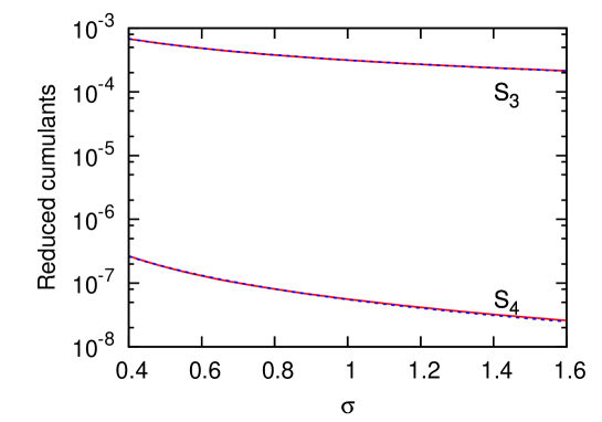
where $k_{3}^{2}=k_{1}^{2}+k_{2}^{2}+2\mu k_{1}k_{2}$. Figure 1 (upper curve) shows the cumulant $S_{3}$ as a function of $\sigma_{R}$ in the mass range $10^{13}-10^{16}\phantom{.}h^{-1}$Mpc. On these scales, the weak scale-dependence in $S_{3}$ can be accurately fitted by a simple formula

$$S_{3}\simeq{3.15\times 10^{-4}\times f_{\mbox{\scriptsize NL}}\over\sigma_{R}^{0.838}},$$ (21)

with sub-percent accuracy. This fitting formula offers an easy way to calculate the observational signatures of $f_{\mbox{\scriptsize NL}}$ without resorting to the integrals in (20).

Figure 1.— Solid lines show the reduced cumulants $S_{3}$ and $S_{4}$ for $f_{\mbox{\scriptsize NL}}=1$ and $g_{\mbox{\scriptsize NL}}=1$ as a function $\sigma(M)$, with mass $M$ ranging between $10^{13}-10^{16}\,h^{-1}M_{\sun}$. Higher values of $f_{\mbox{\scriptsize NL}}$ and $g_{\mbox{\scriptsize NL}}$ scale multiplicatively. The overlapping dashed lines show the fitting formulae given by equations (21) and (25).

3.2. $g_{\mbox{\scriptsize{NL}}}$

If $f_{\mbox{\scriptsize NL}}=0$, we can similarly derive the leading-order relation between $g_{\mbox{\scriptsize NL}}$ and the excess kurtosis

$$\sigma^{6}S_{4}(R) = {3\over 32\pi^{3}}g_{\mbox{\scriptsize NL}}\left(\prod_{i=1}^{3}\int_{0}^{\infty}{dk_{i}\over k_{i}}\phantom{.}A(k_{i})\mathcal{P}(k_{i})\int_{-1}^{1}\!\!d\mu_{i}\int_{0}^{2\pi}\!\!d\phi_{i}\right)A(k_{4})\left[1+3{P_{\phi}(k_{4})\over P_{\phi}(k_{3})}\right],$$ (22)

where

$$k_{4} \equiv \left(k_{1}^{2}+k_{2}^{2}+k_{3}^{2}+2k_{1}k_{2}\Theta_{12}+2k_{2}k_{3}\Theta_{23}+2k_{1}k_{3}\Theta_{13}\right)^{1/2},$$ (23)

$$\Theta_{ij} \equiv \left[(1-\mu_{i}^{2})(1-\mu_{j}^{2})\cos(\phi_{i}-\phi_{j})+\mu_{i}\mu_{j}\right]^{1/2}.$$ (24)

The result of this integration is shown as the lower curve in figure 1. As before, we found a fitting formula

$$S_{4}\simeq{5.53\times 10^{-8}\times g_{\mbox{\scriptsize NL}}\over{\sigma_{R}^{1.70}}},$$ (25)

accurate on the same mass scale.

In summary, we can easily emulate the effects of $f_{\mbox{\scriptsize NL}}$ and $g_{\mbox{\scriptsize NL}}$ using the fitting formulae (21) and (25) without having to compute the multidimensional integrals (20) and (22). Of course, these formulae depend on the choice the primordial power spectrum as well as the window and transfer functions. The fitting formulae are not expected to be very sensitive to the changes in any one these ingredients.

4. Non-Gaussianity based on $f_{\mbox{\scriptsize NL}}$ and $g_{\mbox{\scriptsize NL}}$ only

Much effort has been placed into using the parameters $f_{\mbox{\scriptsize NL}}$ and $g_{\mbox{\scriptsize NL}}$ to specify the deviation of the primordial distribution from Gaussianity. As shown in the previous section, these parameters correspond, at leading order, to deviations from Gaussianity in the 3rd and 4th moments of the distribution. It is important to examine if one can consistently parametrize a non-Gaussian distribution in this way without having to worry about deviations in the higher-order moments. We shall demonstrate that this cannot be the case.

The objective here is to reconstruct the pdf of density fluctuations given a sequence of moments $\{\alpha_{n}\equiv\langle\delta_{R}^{n}\rangle,n=0,1,2\ldots\}$, which, in practice, can be estimated from galaxy-survey data (Cappi & Maurogordato, 1995; Kurokawa et al., 1999). This is the classic moment problem which has been studied in great detail, beginning with the pioneering work of Stieltjes in 1894 and Hamburger in 1920 (see Kjeldsen (1993) for a historical review). In general, there is no guarantee that the resulting pdf will be non-negative, or, indeed, that a solution exists at all. A useful theorem regarding the existence of a solution to the Hamburger moment problem, i.e. when the pdf is defined on $(-\infty,\infty)$, is the following:

Theorem (Existence of solution to the Hamburger moment problem).

The sequence $\{\alpha_{n},n=0,1,2\ldots\}$ corresponds to moments of a non-negative pdf if and only if the determinants

$$D_{n}=\begin{vmatrix}\alpha_{0}&\alpha_{1}&\alpha_{2}&\ldots&\alpha_{n}\\ \alpha_{1}&\alpha_{2}&\alpha_{3}&\ldots&\alpha_{n+1}\\ \alpha_{2}&\alpha_{3}&\alpha_{4}&\ldots&\alpha_{n+2}\\ \vdots&\vdots&\vdots&\vdots&\vdots\\ \alpha_{n}&\alpha_{n+1}&\alpha_{n+2}&\ldots&\alpha_{2n}\end{vmatrix},\phantom{.}\phantom{.}\phantom{.}n=0,1,2\ldots$$ (26)

are all non-negative.

See Shohat & Tamarkin (1963) or Akheizer (1965) for proof.

Let us consider the standardised distribution of $x=\delta_{R}/\sigma_{R}$, so that $\alpha_{0}=1,\alpha_{1}=0$ and $\alpha_{2}=1$. Let us also suppose (as is implicit in some previous works) that non-Gaussianity weakly manifests in the skewness and kurtosis only (therefore $\alpha_{3}$ is close to 0 and $\alpha_{4}$ is close to 3). Higher moments are taken to be identical to those of the normal distribution

$$\alpha_{n}={\begin{cases}(n-1)!!=1\cdot 3\cdot 5\cdots(n-1),&\phantom{.}n\mbox{ even}\\ 0,&\phantom{.}n\mbox{ odd}\end{cases}}\quad(n\geq 5).$$ (27)

The expressions for $D_{n}$ up to $n=6$ are given below. For convenience, we write $\mathsf{s}=\alpha_{3}$ (skewness) and $\mathsf{k}=\alpha_{4}-3$ (excess kurtosis).

$$D_{3} = \mathsf{k}-\mathsf{s}^{2}+2,$$

$$D_{4} = -\mathsf{k}^{3}-8\mathsf{k}^{2}-6\mathsf{k}-3\mathsf{k}\mathsf{s}^{2}-24\mathsf{s}^{2}+\mathsf{s}^{4}+12,$$

$$D_{5} = \mathsf{k}^{5}+15\mathsf{k}^{4}-60\mathsf{k}^{3}-750\mathsf{k}^{2}+360\mathsf{k}-45\mathsf{k}\mathsf{s}^{2}+45\mathsf{k}^{2}\mathsf{s}^{2}-1890\mathsf{s}^{2}+105\mathsf{s}^{4}+288,$$

$$D_{6} = 945\mathsf{k}^{5}+11025\mathsf{k}^{4}-80100\mathsf{k}^{3}-324000\mathsf{k}^{2}-43200\mathsf{k}-132300\mathsf{k}\mathsf{s}^{2}+31500\mathsf{k}^{2}\mathsf{s}^{2}-518400\mathsf{s}^{2}+99225\mathsf{s}^{4}+34560.$$

Note that for the Gaussian distribution ($\mathsf{s}=\mathsf{k}=0$), these $D_{n}$’s are all positive as expected.

Figure 2.— Regions in which the determinant $D_{n}\geq 0$ [see theorem (26)]. The horizontal axis shows $\sigma S_{3}$ (skewness) and the vertical axis shows $\sigma^{2}S_{4}$ (excess kurtosis). The regions correspond to $n=5$ (outermost ellipse) to $n=10$ (innermost ellipse). The regions are nested, co-tangential and converge towards the origin as $n\rightarrow\infty$. The latter fact implies that there is no well-defined non-Gaussian pdf that can be described by deviations in the skewness and kurtosis alone.

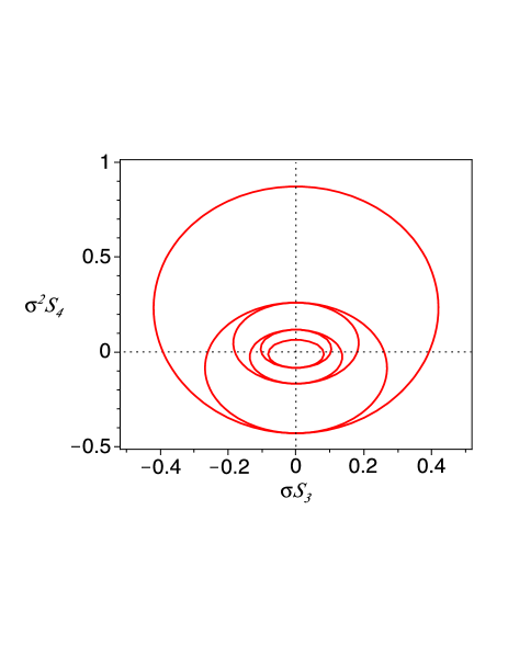
The condition $D_{n}\geq 0$ always describes a closed region in the $(\mathsf{s},\mathsf{k})$ plane containing the origin and bounded by the curve $D_{n}=0$. Figure (2) shows these regions for $n=5$ (outermost ellipse) to $n=10$ (innermost ellipse). To make a connection with later sections, we have labelled the axes as $(\sigma S_{3},\sigma^{2}S_{4})$, where

$$\sigma S_{3}=\mathsf{s},\quad\sigma^{2}S_{4}=\mathsf{k},$$ (28)

as can be easily shown using relation (18)-(19) (to avoid cluttering we sometimes write $\sigma$ to mean $\sigma_{R}$). As $n$ increases, the region corresponding to $D_{n}\geq 0$ becomes smaller. Interestingly, the regions for any two consecutive values of $n$ are nested and co-tangential. One can continue inductively this way to find that as $n\rightarrow\infty$, the ellipses converge to the origin, implying that there is no room for any deviation from Gaussianity. We conclude that deviations in the skewness and kurtosis alone cannot consistently parametrize a non-Gaussian pdf.

The upshot of all this is that $f_{\mbox{\scriptsize NL}}$ and $g_{\mbox{\scriptsize NL}}$ by themselves cannot completely describe a non-Gaussian pdf. Information on higher-order correlation must be available for the pdf to be well defined.

5. The Edgeworth Expansion

As described in the Introduction, the Edgeworth expansion is a convenient way to express a weakly non-Gaussian pdf as a series comprising its cumulants. Suppose that we only have estimates on $f_{\mbox{\scriptsize NL}}$ and $g_{\mbox{\scriptsize NL}}$, and no higher-order non-Gaussianity. The result of the previous section shows that the resulting pdf cannot be non-negative.

Nevertheless, this result only holds if we use an infinite number of cumulants in the reconstruction of the pdf. This is equivalent to having an infinite number terms in the Edgeworth expansion. In numerical implementations, however, one truncates the Edgeworth expansion after a finite number of terms. As we will see shortly, it now becomes possible to describe an entirely non-negative pdf with only $f_{\mbox{\scriptsize NL}}$ and $g_{\mbox{\scriptsize NL}}$, circumventing the result of the previous section. The disadvantage of the truncation is, of course, that the cumulants of the reconstructed pdf may not correspond exactly to those of the actual pdf, and thus the statistical significance of $f_{\mbox{\scriptsize NL}}$ and $g_{\mbox{\scriptsize NL}}$ is somewhat weakened. For very short series of just a few terms, the interpretations of $f_{\mbox{\scriptsize NL}}$ as skewness and $g_{\mbox{\scriptsize NL}}$ as excess kurtosis are especially dubious.

Given information on a finite number of cumulants, we shall investigate the sensitivity of the resulting pdf to the number of terms in the Edgeworth expansion. This sensitivity has been alluded to by several works in the literature (Juszkiewicz et al., 1995; LoVerde et al., 2008; Desjacques et al., 2008), though we believe that our analysis goes beyond those works. In particular, we shall argue that the truncated series cannot be used to deduce results for negative $g_{\mbox{\scriptsize NL}}$, unless some higher-order non-Gaussianities are known.

5.1. The Petrov development

In this paper, we shall be using the form of the Edgeworth series given by Petrov (1975), who gave a method of calculating the Edgeworth series to arbitrarily high order. Given a non-Gaussian pdf with zero mean and variance $\sigma_{R}^{2}$, we can express its deviation from Gaussianity as a product of the normal distribution and a Taylor series in $\sigma_{R}$:

$$p(\delta_{R})=N(\delta_{R})\left[1+\sum_{s=1}^{\infty}\sigma_{R}^{s}E_{s}\!\!\left(\delta_{R}\over\sigma_{R}\right)\right],$$ (29)

where $N(\delta_{R})$ is the normal distribution

$$N(\delta_{R})={1\over\sigma_{R}\sqrt{2\pi}}\exp\left(-\delta_{R}^{2}\over 2\sigma_{R}^{2}\right),$$ (30)

and the coefficients $E_{s}$ in the Taylor series are given by

$$E_{s}\left(\nu\right) = \!\sum_{\{k_{m}\}}\left[H_{s+2r}\!\left(\nu\right)\prod_{m=1}^{s}{1\over k_{m}!}\left(S_{m+2}\over(m+2)!\right)^{k_{m}}\!\right],\phantom{.}$$ (31)

$$\mbox{where}\quad\nu \equiv {\delta_{R}\over\sigma_{R}}.$$

We now explain the various components of the coefficient (31). Firstly, the sum is taken over all distinct sets of non-negative integers $\{k_{m}\}_{m=1}^{s}$ satisfying the Diophantine equation

$$k_{1}+2k_{2}+\ldots+sk_{s}=s.$$ (32)

We also define

$$r\equiv k_{1}+k_{2}+\ldots+k_{s}.$$ (33)

Next, the function $H_{n}(\nu)$ is the Hermite polynomial of degree $n$. They can be obtained by the Rodrigues’ formula

$$H_{n}(\nu)=(-1)^{n}e^{\nu^{2}/2}{d{{}^{n}}\over d{\nu^{n}}}\left(e^{-{\nu^{2}/2}}\right).$$ (34)

For example, $H_{0}(\nu)=1$ and $H_{1}(\nu)=\nu$. Higher order polynomials can be easily obtained via the recurrence relation

$$H_{n+1}(\nu)=\nu H_{n}(\nu)-nH_{n-1}(\nu).$$ (35)

Note that if $p(\delta_{R})$ is Gaussian, the cumulants of order $\geq 3$ vanish identically, and so do the expansion coefficients (31), as one might expect.

5.2. Validity of the truncated series

The Edgeworth expansion takes, as input, a sequence of cumulants $\{S_{n}\}$ which are combined with polynomials of various degrees up to order $N$. Therefore, when using the Edgeworth expansion, there are two factors which will determine its accuracy, namely 1) the number of available cumulants, and 2) the order $N$. These two issues are separate in the sense that it is possible to expand the Edgeworth series to arbitrarily high order given a limited number of cumulants. Both these issues must be analysed to properly monitor the sources of error.

5.2.1 Linear truncation

When the Edgeworth series (29) is truncated at linear order in $\sigma_{R}$, the resulting pdf is given by

$$p(\nu)=N(\nu)\left[1+{\sigma_{R}S_{3}\over 6}(\nu^{3}-3\nu)\right],$$ (36)

where $\nu\equiv\delta_{R}/\sigma_{R}$ as before. Observe that if $S_{3}>0$, a sufficiently large negative $\nu$ gives $p(\nu)<0$ and, similarly, if $S_{3}<0$, a sufficiently large positive $\nu$ gives $p(\nu)<0$. For instance, if $|S_{3}|=0.1$, $p(\nu)$ becomes negative as early as $|\nu|\simeq 3$. This implies that a linear truncation of the Edgeworth series is highly suspect and is certainly not suitable for calculating, for instance, the mass function whereby high values of density fluctuations are involved.

5.2.2 Quadratic truncation

The Edgeworth series truncated at quadratic order in $\sigma_{R}$ yields

$$p(\nu)=N(\nu)\left[1+{\sigma_{R}S_{3}\over 6}H_{3}(\nu)+\sigma_{R}^{2}\left({S_{4}\over 24}H_{4}(\nu)+{S_{3}^{2}\over 72}H_{6}(\nu)\right)\right].$$ (37)

We wish to determine the combination of $S_{3}$ and $S_{4}$ such that $p(\nu)$ is non-negative. The numerical evaluation of $p(\nu)$ over a grid of $S_{3}$ and $S_{4}$ is shown in figure 3. In the figure, we mark points for which $p(\nu)>0$ in the $(\sigma_{R}S_{3},\sigma_{R}^{2}S_{4})$ plane, in the domain $\nu\in[-20,20]$. This reveals a closed region in which $p(\nu)>0$. In fact, the bounding envelope can be found analytically by setting $p(\nu)=p^{\prime}(\nu)=0$, but the resulting equation has a very complicated parametric form which we shall not show here. For details of this technique see Jondeau & Rockinger (2001).

Figure 3.— Validity of the quadratic Edgeworth expansion (37). The shaded region corresponds to the combination of $S_{3}$ and $S_{4}$ for which there exists a non-negative pdf over the entire real line. See the text for further discussions and proof of the bound $0\leq\sigma^{2}S_{4}\leq 4$.

A curious feature of figure 3 is that the excess kurtosis, $\sigma^{2}S_{4}$, is limited to a small, non-negative range. We can prove this as follows. Setting $S_{3}=0$, the quadratic series can be written as

$${p(\nu)\over N(\nu)}=1+{\sigma_{R}^{2}S_{4}\over 24}\left[(\nu^{2}-3)^{2}-6\right].$$ (38)

This expression clearly achieves the minimum when $\nu^{2}-3=0$. Requiring the minimum to be non-negative establishes the upper bound $\sigma^{2}S_{4}\leq 4$. Next, if $S_{4}<0$, the quartic expression is unbounded from below and so the pdf will be negative for some large $x$. Thus, we must have $0\leq\sigma^{2}S_{4}\leq 4$

The bound for $\sigma S_{3}$ is more difficult to establish and we shall not go into the detail here. We simply note since an analytic expression describing the shaded region in figure 3 exists, the region in fact represents combinations of $S_{3}$ and $S_{4}$ ($f_{\mbox{\scriptsize NL}}$ and $g_{\mbox{\scriptsize NL}}$) for which the pdf is non-negative on the entire real line and not just in [-20,20]. For higher-order truncations, it becomes increasingly difficult to find such a region, as expected given the conclusion in section 4

Figure 4.— Validity of the Edgeworth expansion in the $(\sigma S_{3},\sigma^{2}S_{4})$ plane for $\nu\equiv\delta/\sigma$ in the range $[-5,5]$ (column on the left) and $[-20,20]$ (right) with the series is expanded up to (from top to bottom) $\sigma^{3}$, $\sigma^{5}$, $\sigma^{10}$ and $\sigma^{20}$. Only deviations in the skewness and the excess kurtosis are taken into account, with no higher-order non-Gaussianities. Points correspond to those combinations resulting in a non-negative pdf. See the text for further discussions on how the Edgeworth expansion may be properly used to produce non-negative pdfs.

5.2.3 Higher-order truncations

Figure 5.— Including non-zero 6th and 8th cumulants ($S_{6}$ and $S_{8}$) opens up the region of validity of the truncated Edgeworth series to include models with $S_{4}<0$ (compare with figure 4, 3rd row, right column). Only points with $S_{4}<0$ are shown. For all these points, the 8th cumulant, $S_{8}$, is positive, as explained in the text.

Figure 4 shows the same set of axes as figure 3 with the Edgeworth series now expanded up to terms of order $\sigma^{3}$, $\sigma^{5}$, $\sigma^{10}$ and $\sigma^{20}$ (top row to bottom row). In producing these figures, we have set the rest of the cumulants to zero. This is roughly equivalent to parametrizing the non-Gaussianity by $f_{\mbox{\scriptsize NL}}$ and $g_{\mbox{\scriptsize NL}}$ only. Note that if $n$ is odd, the series up to $n$ terms performs significantly worse than one with even $n$. This is simply because odd (Hermite) polynomials are not positive definite, whereas even ones are, provided the coefficients are properly chosen. When scanning over a sufficiently large range of $\nu$, an odd-ordered Edgeworth expansion will not produce any well-defined pdf whatsoever.

The sensitivity of the regions to the range of $\nu$ considered is clearly seen in the difference between the column on the left (in which $p(\nu)$ is only required to be non-negative for $|\nu|<5$) and on the right ($|\nu|<20$). As the range of $\nu$ increases, the cluster of points shrinks as it becomes increasingly difficult to find a closed region with $p(\nu)>0$.

Observe that for $\nu\in[-20,20]$, very few models with negative $S_{4}$ (i.e.$\phantom{.}g_{\mbox{\scriptsize NL}}<0$) are produced. In fact, if the range of $\nu$ is sufficiently large, no models with negative $S_{4}$ are produced at all. A simple explanation for this is as follows. If the highest non-zero cumulant of a non-Gaussian distribution is $S_{4}$, then, for large $\nu$, the Edgeworth series expanded to $n$ terms is of order $S_{4}\nu^{n}$. Hence, if $S_{4}<0$, a sufficiently large $\nu$ will render the expansion negative regardless of the value of $n$.

Therefore, it is necessary that higher-order non-Gaussianities are taken into account when modelling a non-Gaussian distribution with $g_{\mbox{\scriptsize NL}}<0$. For instance, including nonzero cumulants $S_{6}$ and $S_{8}$ opens up the parameter space to those with $S_{4}<0$, as shown in figure 5.

In summary, the Edgeworth series should be expanded up to even order in $\sigma_{R}$ to produce a well-defined pdf. The highest cumulant in that case is restricted to non-negative values. The Edgeworth expansion therefore can describe models with $g_{\mbox{\scriptsize NL}}<0$ if and only if cumulants of order at least $6$ or higher are included. If $g_{\mbox{\scriptsize NL}}=0$ and non-Gaussianity is parametrized by $f_{\mbox{\scriptsize NL}}$ only, the Edgeworth expansion is odd-ordered and the resulting pdf is not well-defined.

Although we have assumed that non-Gaussianity is characterised purely by the ‘local’ $f_{\mbox{\scriptsize NL}}$ and $g_{\mbox{\scriptsize NL}}$ parameters, the results in this section (as summarised in figures 3-5) have been established in terms of the cumulants, $S_{n}$, and so they hold even if there are other types of non-Gaussianity present. The only difference in this case is that it will be more complicated to translate the cumulants into $f_{\mbox{\scriptsize NL}}$-type parameters. For instance, $S_{3}$ will now comprise a mixture of local and non-local contributions

$$S_{3}=f_{\mbox{\scriptsize NL}}^{\mbox{\scriptsize{local}}}\mathcal{I}_{1}+f_{\mbox{\scriptsize NL}}^{\mbox{\scriptsize{nonlocal}}}\mathcal{I}_{2},$$ (39)

where $\mathcal{I}_{1}$ and $\mathcal{I}_{2}$ are some integral expressions. See LoVerde et al. (2008); Desjacques & Seljak (2010) for the expressions for $\mathcal{I}_{2}$ in the case where non-Gaussianity is of the so-called folded or equilateral-triangle type.

Having understood how to produce well-defined non-Gaussian pdfs using the Edgeworth expansion, we shall now look at two applications, namely, the non-Gaussian prediction for abundances of clusters and voids. In what follows, we shall focus on the case where $f_{\mbox{\scriptsize NL}}=0$ and $g_{\mbox{\scriptsize NL}}>0$.

6. Abundance of massive clusters

Large-scale structures are sensitive to primordial non-Gaussianity on scales much smaller than the CMB (see Desjacques & Seljak (2010) for a recent review). On these scales, non-Gaussianity can manifest in the changes in cluster number count and its redshift dependence (Lucchin & Matarrese, 1988; Robinson & Baker, 2000; LoVerde et al., 2008; Oguri, 2009) as well as a scale-dependent halo bias (Dalal et al., 2008; Matarrese & Verde, 2008; Wands & Slosar, 2009). In this work, we use the Edgeworth approach, in its correct formalism, together with Press-Schechter theory to study the effect of non-zero $g_{\mbox{\scriptsize NL}}$ on the number density of massive clusters. Redshift dependence and the effects on the correlation function will be examined in a later publication.

6.1. Press-Schechter theory

Let $n(M)$ be the number density of collapsed objects of mass above $M$. Press-Schechter theory (Press & Schechter, 1974) gives the differential number density of collapsed objects as

$${d{n}\over d{M}}=-2{\rho_{m}\over M}{d{}\over d{M}}\int_{\delta_{c}/\sigma(M)}^{\infty}p(\nu,M)d\nu,$$ (40)

where $p(\nu,M)$ is the pdf smoothed by a window function containing mass $M$ and $\delta_{c}\approx 1.686$ is the threshold overdensity for spherical collapse. For a non-Gaussian pdf , Grossi et al. (2009) suggest that a good fit to N-body simulations can be obtained by using the Press-Schechter mass function modified by the replacement

$$\delta_{c}\rightarrow 0.866\phantom{.}\delta_{c},$$ (41)

(see Maggiore & Riotto (2009b) for a possible theoretical origin.) We make this replacement in our calculations.

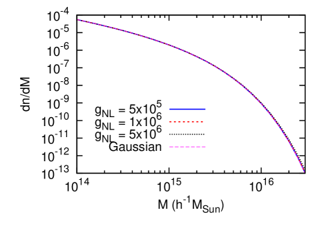
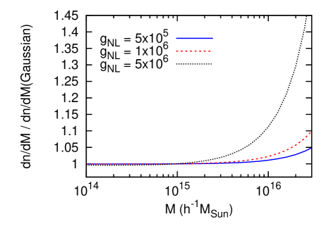
Figure 6 shows the changes in $dn/dM$ for a range of non-Gaussian models with $g_{\mbox{\scriptsize NL}}=5\times 10^{5},1\times 10^{6}$ and $5\times 10^{6}$ ($f_{\mbox{\scriptsize NL}}=0$ in all cases). In these calculations, we keep the Edgeworth expansion up to $10$ terms and check that $p(\nu)>0$ at least in the range $\nu\in[-20,20]$. Outside this range, the $p(\nu)$ is sufficiently small and the contribution to the cluster abundance on this mass scale is negligible (note that for the normal distribution, $N(20)\sim 10^{-88}$). The values of $g_{\mbox{\scriptsize NL}}$ have been chosen to stay within the region of validity (see figure 4). In our case, we require $0\leq\sigma^{2}S_{4}\lesssim 0.6$, corresponding roughly to $0\lesssim g_{\mbox{\scriptsize NL}}\lesssim\mathcal{O}(10^{8})$.

The general effect of $g_{\mbox{\scriptsize NL}}>0$ is a boost in the number density of the most massive objects, although a significant boost requires the magnitude of $g_{\mbox{\scriptsize NL}}$ to exceed the CMB-derived bound of Vielva & Sanz (2010). For instance, abundance of objects of mass $\sim 10^{16}M_{\sun}$ (corresponding to the most massive clusters) is increased by about 10% for $g_{\mbox{\scriptsize NL}}=5\times 10^{6}$. Nevertheless, values of $g_{\mbox{\scriptsize NL}}$ of this magnitude has recently been proposed by Enqvist et al. (Enqvist et al., 2010) to explain the observed excess of massive clusters. Until there is a larger compilation of massive clusters, the possibility of non-Gaussianity with $g_{\mbox{\scriptsize NL}}\sim\mathcal{O}(10^{6})$ remains a viable.

Figure 6.— Left: The differential number density $dn/dM$ as a function of mass scale $M$ for models with $g_{\mbox{\scriptsize NL}}=5\times 10^{5},1\times 10^{6}$ and $5\times 10^{6}$ ($f_{\mbox{\scriptsize NL}}=0$). The number density of massive clusters increases with $g_{\mbox{\scriptsize NL}}$. Right: Ratios between the non-Gaussian and Gaussian number densities.

6.2. Sensitivity to truncation

Increasing the number of terms in the Edgeworth expansion does not change the pdf drastically. However, because the mass function is extremely sensitive to the exponential tail of the distribution, it is imperative that one keeps as many terms as practically possible in the Edgeworth expansion. Exactly how many terms are required will depend on a combination of factors such as the range of scales of interest or the redshift at which the calculations are made.

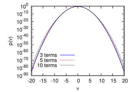
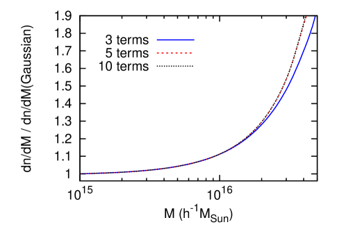
Figure 7 demonstrates the sensitivity of the Edgeworth expansion to the truncation order. The panel on the left shows the pdf for a distribution with $g_{\mbox{\scriptsize NL}}=5\times 10^{6}$ (with higher-order cumulants again equal $0$) and $R=8h^{-1}$Mpc. The various lines correspond to the number of terms in the Edgeworth expansion. For $\nu\sim\mathcal{O}(1)$, the pdfs lie almost exactly on top of one another, diverging only at the tail ends. However, when dealing with extreme-mass objects, keeping just a few terms in the Edgeworth series is inadequate, as seen in the panel on the right. Here, the ratio of the non-Gaussian number density $dn/dM$ and the Gaussian value can change by $10\%$ as the number of terms increases from 3 to 5 on mass scales beyond $10^{16}M_{\sun}$. Comparing with figure 6, we conclude that fitting the observed abundance of massive clusters using a low truncation order would lead to a spuriously high value of $g_{\mbox{\scriptsize NL}}$ and vice versa.

We note that is likely that the sensitivity to the truncation order could increase significantly with redshift. We shall address this issue in a forthcoming work.

Figure 7.— The sensitivity of the Edgeworth series to the truncation order Left: the pdf $p(\nu)$ for models with $g_{\mbox{\scriptsize NL}}=5\times 10^{6}$. Increasing the number of terms in the Edgeworth expansion from 3 to 10 changes the pdf at high values of $|\nu|$ only by a tiny amount (note the logarithmic scale on the vertical axis). Right: the effect of increasing the number of terms in the Edgeworth series on the cluster abundance $dn/dM$. A fifth (and higher) order expansion can give $dn/dM$ (shown here as a ratio to the Gaussian value) higher than a third-order truncation by up to $10\%$ at high $M$. Further increment in the number of terms has no discernible effect on the abundance in this mass range.

7. Abundance of voids

Primordial non-Gaussianity also changes the abundance of underdense regions, i.e. cosmic voids. An estimate of void abundance can be computed by a simple extension of the Press-Schechter formalism (Kamionkowski et al., 2009; Biswas et al., 2010), although there are more sophisticated methods based on the void probability function (White, 1979) or the eigenvalues of the tidal tensor (Doroshkevich, 1970; Lam et al., 2009). Presently, we shall use the Press-Schechter approach with the Edgeworth expansion to calculate the effect of $g_{\mbox{\scriptsize NL}}$ on the void abundance.

A void can be defined as an isolated region in which $-1\leq\delta\leq\delta_{v}$, where $\delta_{v}$ is some threshold underdensity. Simulations carried out by Shandarin et al. (2006),Park & Lee (2007) and Colberg et al. (2008) suggest $\delta_{v}\approx-0.8$. Linearly extrapolating this value to $z=0$ using the fitting formula of Mo & White (1996) gives $\delta_{v}=-2.75$.

Let $\mbox{Prob}_{<\delta_{v}}(\mathbf{x})$ be the probability that $\delta<\delta_{v}$ at $\mathbf{x}$. Since $\mbox{Prob}_{<\delta_{v}}=1-\mbox{Prob}_{>\delta_{v}}$, differentiating this expression with respect to $R$ shows that the analog of equation 40 for voids can simply be obtained by the replacement $\delta_{c}\rightarrow\delta_{v}$ and a change in the overall sign.

Figure 8.— Left: The differential void abundance $dn/dR$ as a function of scale $R$ for models with $g_{\mbox{\scriptsize NL}}=5\times 10^{5},1\times 10^{6}$ and $5\times 10^{6}$ ($f_{\mbox{\scriptsize NL}}=0$). The number density of large voids increases with $g_{\mbox{\scriptsize NL}}$. Right: Ratios between the non-Gaussian and Gaussian void abundances, showing the factor of enhancement. Voids appear to respond much more sensitively to $g_{\mbox{\scriptsize NL}}$ compared to clusters (see figure 6).

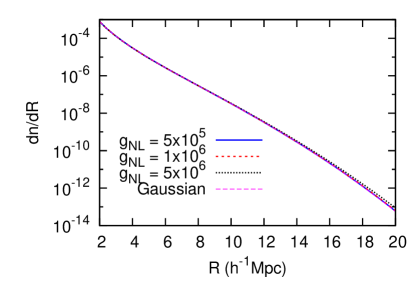
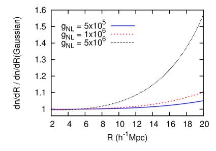
Figure 8 shows the differential number density $dn/dR$ for models in which $g_{\mbox{\scriptsize NL}}=5\times 10^{5},1\times 10^{6}$ and $5\times 10^{6}$ , plotted against the smoothing scale $R$. By increasing $g_{\mbox{\scriptsize NL}}$, the void abundance is enhanced and responds much more sensitively than the cluster abundance (compare figures 6 and 8). For example, in the extreme case where $g_{\mbox{\scriptsize NL}}=5\times 10^{6}$, at $R=20\phantom{.}h^{-1}\mbox{Mpc}$ ($M\approx 10^{16}\phantom{.}h^{-1}M_{\sun}$), the enhancement in the differential abundance compared to the Gaussian prediction is roughly $10\%$ for clusters, but as large as $60\%$ for voids. This suggests that large voids may be a more sensitive probe of primordial non-Gaussianity than massive clusters, although a more careful calculation is needed to confirm this.

Another interesting observation is that $g_{\mbox{\scriptsize NL}}>0$ enhances both cluster and void abundances. This is in contrast with the effect of $f_{\mbox{\scriptsize NL}}>0$, which enhances the number density of clusters, but suppresses the number density of voids (Lam et al., 2009; Kamionkowski et al., 2009). Comparing the abundances of clusters and voids may offer a way to probe any asymmetry in the distribution of density fluctuations.

8. Conclusions

The key results in this paper are as follows

• We clarified the statistical meaning of the local non-Gaussianity parameters $f_{\mbox{\scriptsize NL}}$ and $g_{\mbox{\scriptsize NL}}$, which, at leading order, are proportional to the skewness and excess kurtosis of the distribution of density fluctuations. These relations are in the form of multi-dimensional integrals, which can be fitted by simple formulae (21) and (25). They are accurate on the mass scale $10^{13}-10^{16}\phantom{.}M_{\sun}$.

• We showed that the information in $f_{\mbox{\scriptsize NL}}$ and $g_{\mbox{\scriptsize NL}}$ is insufficient for a reconstruction of the pdf of density fluctuations. Using a theorem from the classical Hamburger moment problem, we showed that there is no positive pdf which deviates from Gaussianity only in the 3rd and 4th moments.

• We studied the truncated Edgeworth series, emphasising that in this representation, $f_{\mbox{\scriptsize NL}}$ and $g_{\mbox{\scriptsize NL}}$ may not accurately reflect the skewness and excess kurtosis of the reconstructed pdf, especially for shorter truncations. We surveyed the skewness-kurtosis plane for regions of validity (i.e. where the pdf is non-negative) for various truncations of the Edgeworth series. We proved that the Edgeworth expansion can represent a non-negative pdf if it is truncated at even order in $\sigma$, with the highest-order cumulant restricted to non-negative values. In terms of local non-Gaussianity, this means that the Edgeworth series cannot be used to represent models with nonzero $f_{\mbox{\scriptsize NL}}$ without considering nonzero $g_{\mbox{\scriptsize NL}}$ also. It also means that models with $g_{\mbox{\scriptsize NL}}<0$ are not representable by a truncated Edgeworth series unless the non-Gaussian deviation in the 6th moment (or higher) is known.

• Working with a 10th-order Edgeworth series, we calculated the effects of $g_{\mbox{\scriptsize NL}}$ on the cluster number density, $dn/dM$, using the Press-Schechter formalism (see figure 6). The differential abundance of the most massive clusters can increase significantly if $g_{\mbox{\scriptsize NL}}\sim 10^{6}$. We cautioned that the deduced value of $g_{\mbox{\scriptsize NL}}$ from large-scale structures may be spuriously high if the series is prematurely truncated.

• Finally, we extended the Press-Schechter approach to compute the effects of $g_{\mbox{\scriptsize NL}}$ on the abundance of large voids. The void number density is enhanced much more sensitively compared to clusters (figure 8). This could be confirmed by a more sophisticated calculation (e.g. using correlation functions to calculate the void probability distribution). We shall address this issue in a future publication.

acknowledgments

SC is supported by Lincoln College, Oxford. We are grateful to Profs. N. Sugiyama and S. Zaroubi for early discussions that helped inspired this project, to Sergei Blinnikov for sharing his Petrov-Edgeworth code, to Lindsay King and Pedro Ferreira for reading the manuscript, and to Bob Scherrer and the referee for many helpful suggestions. Many thanks also to Shaun Hotchkiss, Sarah Shandera, Qing-Guo Huang, Laura Cayón and Elizabeth Eardley for discussions that led to the improvement of the original version.

References

- Akheizer (1965) Akheizer, N. I. 1965, The classical moment problem and related questions in analysis (New York: Hafner Publishing Company)
- Alishahiha et al. (2004) Alishahiha, M., Silverstein, E., & Tong, D. 2004, Phys. Rev. D, 70, 123505
- Amendola (2002) Amendola, L. 2002, ApJ, 569, 595, arXiv:astro-ph/0107527
- Arkani-Hamed et al. (2004) Arkani-Hamed, N., Creminelli, P., Mukohyama, S., & Zaldarriaga, M. 2004, JCAP, 0404, 001, hep-th/0312100
- Balitskaya & Zolotuhina (1988) Balitskaya, E. O., & Zolotuhina, L. A. 1988, Biometrika, 75, 185
- Bartolo et al. (2004a) Bartolo, N., Komatsu, E., Matarrese, S., & Riotto, A. 2004a, Phys. Rept., 402, 103
- Bartolo et al. (2004b) Bartolo, N., Matarrese, S., & Riotto, A. 2004b, Phys. Rev. D, 69, 043503
- Bernardeau & Kofman (1995) Bernardeau, F., & Kofman, L. 1995, ApJ, 443, 479, arXiv:astro-ph/9403028
- Biswas et al. (2010) Biswas, 1, R., Alizadeh, E., & Wandelt, B. D. 2010, 1002.0014
- Blinnikov & Moessner (1998) Blinnikov, S., & Moessner, R. 1998, A&AS, 130, 193, arXiv:astro-ph/9711239
- Byrnes & Choi (2010) Byrnes, C. T., & Choi, K. 2010, 1002.3110
- Cappi & Maurogordato (1995) Cappi, A., & Maurogordato, S. 1995, ApJ, 438, 507
- Cayon et al. (2010) Cayon, L., Gordon, C., & Silk, J. 2010, 1006.1950
- Chen (2005) Chen, X. 2005, Phys. Rev., D72, 123518
- Chen (2010) ——. 2010, 1002.1416
- Chen et al. (2007) Chen, X., Huang, M.-x., Kachru, S., & Shiu, G. 2007, JCAP, 0701, 002, hep-th/0605045
- Colberg et al. (2008) Colberg, J. M., et al. 2008, 0803.0918
- Dalal et al. (2008) Dalal, N., Dore, O., Huterer, D., & Shirokov, A. 2008, Phys. Rev., D77, 123514, 0710.4560
- D’Amico et al. (2010) D’Amico, G., Musso, M., Noreña, J., & Paranjape, A. 2010, 1005.1203
- Desjacques & Seljak (2010) Desjacques, V., & Seljak, U. 2010, 1006.4763
- Desjacques et al. (2008) Desjacques, V., Seljak, U., & Iliev, I. 2008, 0811.2748
- Doroshkevich (1970) Doroshkevich, A. G. 1970, Astrofizika, 6, 581
- Draper & Tierney (1972) Draper, N. R., & Tierney, D. E. 1972, Biometrika, 59, 463
- Eisenstein & Hu (1998) Eisenstein, D. J., & Hu, W. 1998, ApJ, 496, 605
- Enqvist et al. (2010) Enqvist, K., Hotchkiss, S., & Taanila, O. 2010, 1012.2732
- Grossi et al. (2009) Grossi, M., et al. 2009, Mon. Not. Roy. Astron. Soc., 398, 321
- Jondeau & Rockinger (2001) Jondeau, E., & Rockinger, M. 2001, Journal of Economic Dynamics and Control, 25, 1457
- Juszkiewicz et al. (1995) Juszkiewicz, R., Weinberg, D. H., Amsterdamski, P., Chodorowski, M., & Bouchet, F. 1995, ApJ, 442, 39, arXiv:astro-ph/9308012
- Kamionkowski et al. (2009) Kamionkowski, M., Verde, L., & Jimenez, R. 2009, JCAP, 0901, 010
- Kjeldsen (1993) Kjeldsen, T. H. 1993, Historia Mathematica, 20, 19
- Komatsu et al. (2010) Komatsu, E., et al. 2010, 1001.4538
- Kurokawa et al. (1999) Kurokawa, T., Morikawa, M., & Mouri, H. 1999, A&A, 344, 1
- Lahav & Liddle (2010) Lahav, O., & Liddle, A. R. 2010, 1002.3488
- Lam et al. (2009) Lam, T. Y., Sheth, R. K., & Desjacques, V. 2009, 0905.1706
- Langlois et al. (2008) Langlois, D., Renaux-Petel, S., Steer, D. A., & Tanaka, T. 2008, Phys. Rev. Lett., 101, 061301
- LoVerde et al. (2008) LoVerde, M., Miller, A., Shandera, S., & Verde, L. 2008, JCAP, 0804, 014
- Lucchin & Matarrese (1988) Lucchin, F., & Matarrese, S. 1988, ApJ, 330, 535
- Maggiore & Riotto (2009a) Maggiore, M., & Riotto, A. 2009a, 0903.1249
- Maggiore & Riotto (2009b) ——. 2009b, 0903.1251
- Maggiore & Riotto (2010) ——. 2010, ApJ, 717, 515, 0903.1250
- Matarrese & Verde (2008) Matarrese, S., & Verde, L. 2008, ApJ, 677, L77
- Mo & White (1996) Mo, H. J., & White, S. D. M. 1996, Mon. Not. Roy. Astron. Soc., 282, 347
- Oguri (2009) Oguri, M. 2009, Phys. Rev. Lett., 102, 211301
- Park & Lee (2007) Park, D., & Lee, J. 2007, Phys. Rev. Lett., 98, 081301
- Petrov (1975) Petrov, V. 1975, Ergebnisse der Mathematik und ihrer Grenzgebiete, Vol. 82, Sums of independent random variables (Berlin: Springer-Verlag)
- Press & Schechter (1974) Press, W. H., & Schechter, P. 1974, ApJ, 187, 425
- Rigopoulos et al. (2006) Rigopoulos, G. I., Shellard, E. P. S., & van Tent, B. J. W. 2006, Phys. Rev., D73, 083522
- Robinson & Baker (2000) Robinson, J., & Baker, J. E. 2000, MNRAS, 311, 781, arXiv:astro-ph/9905098
- Sasaki et al. (2006) Sasaki, M., Väliviita, J., & Wands, D. 2006, Phys. Rev. D, 74, 103003
- Sefusatti et al. (2009) Sefusatti, E., Liguori, M., Yadav, A. P. S., Jackson, M. G., & Pajer, E. 2009, JCAP, 0912, 022
- Shandarin et al. (2006) Shandarin, S., Feldman, H. A., Heitmann, K., & Habib, S. 2006, Mon. Not. Roy. Astron. Soc., 367, 1629
- Shohat & Tamarkin (1963) Shohat, J., & Tamarkin, J. 1963, Mathematical Surveys and Monographs, Vol. 1, The Problem of Moments (American Mathematical Society)
- Vielva & Sanz (2010) Vielva, P., & Sanz, J. L. 2010, MNRAS, 404, 895
- Wands & Slosar (2009) Wands, D., & Slosar, A. 2009, Phys. Rev., D79, 123507
- Weinberg (2008) Weinberg, S. 2008, Cosmology (Oxford University Press)
- White (1979) White, S. D. M. 1979, MNRAS, 186, 145