Transverse flow in thin superhydrophobic channels

Abstract

We provide some general theoretical results to guide the optimization of transverse hydrodynamic phenomena in superhydrophobic channels. Our focus is on the canonical micro- and nanofluidic geometry of a parallel-plate channel with an arbitrary two-component (low-slip and high-slip) coarse texture, varying on scales larger than the channel thickness. By analyzing rigorous bounds on the permeability, over all possible patterns, we optimize the area fractions, slip lengths, geometry and orientation of the surface texture to maximize transverse flow. In the case of two aligned striped surfaces, very strong transverse flows are possible. Optimized superhydrophobic surfaces may find applications in passive microfluidic mixing and amplification of transverse electrokinetic phenomena.

Introduction.– Hydrophobic solid surfaces with special textures can exhibit greatly enhanced (“super”) properties, compared to analogous flat or slightly disordered surfaces Quere (2005). If the liquid follows the topological variations of the surface (the Wenzel state), roughness can not only significantly increase hydrophobicity, but can also lead to a giant drop’s adhesion. In contrast, when the recessed regions of the texture are filled with gas (the Cassie state), roughness can dramatically lower the ability of drops to stick and produce remarkable liquid mobility. At the macroscopic scale, such surfaces are “self-cleaning”, causing droplets to roll (rather than slide) under gravity and rebound (rather than spread) upon impact. At the microscopic scale, superhydrophobic surfaces could revolutionize microfluidic lab-on-a-chip systems Stone et al. (2004); Squires and Quake (2005), which are becoming widely used in biotechnology. The large effective slip of superhydrophobic surfaces Ybert et al. (2007); Feuillebois et al. (2009) compared to simple, smooth channels Vinogradova et al. (2009); Vinogradova and Yakubov (2003); Cottin-Bizonne et al. (2005) can greatly lower the viscous drag of thin microchannels and reduce the tendency for clogging or adhesion of suspended analytes. Superhydrophobic surfaces can also amplify electrokinetic pumping or energy conversion in microfluidic devices, if diffuse charge in the liquid extends over the gas regions  Squires (2008); Bahga et al. (2010); Huang et al. (2008).

Superhydrophobic surfaces in nature (e.g. the lotus leaf) are typically isotropic, but microfabrication has opened the possibility of highly anisotropic textures Quere (2008). The effective hydrodynamic slip Bazant and Vinogradova (2008); Stone et al. (2004); Kamrin et al. (2010) (or electro-osmotic mobility Bahga et al. (2010)) of anisotropic textured surfaces is generally tensorial, due to secondary flows transverse to the direction of the applied pressure gradient (or electric field Ajdari (2001)). In the case of grooved no-slip surfaces (Wenzel state), transverse viscous flows have been analyzed for small height variations Stroock et al. (2002a) and thick channels Wang (2003), and herringbone patterns have been designed to achieve passive chaotic mixing during pressure-driven flow through a microchannel Stroock et al. (2002b); Stroock and McGraw (2004); Villermaux et al. (2008). Convection is often required to mix large molecules, reagents, or cells in lab-on-a-chip devices, and passive mixing by textured surfaces can be simpler and more robust than mechanical or electrical actuation. In principle, these effects may be amplified by hydrodynamic slip (Cassie state) and large amplitude roughness (Wenzel state), but we are not aware of any prior work.

Figure 1: Sketch of a thin channel of thickness $h(x,y)$ with notation for directions along the plates. In the Wenzel state the liquid would conform the solid surface, but in the Cassie state it remains free-standing at the top of the roughness

In this Letter, we present some general theoretical results to guide the optimization of transverse hydrodynamic phenomena in a thin superhydrophobic channel. We consider an arbitrary coarse texture, varying on scales larger than the channel thickness, and optimize its orientation and geometry to maximize pressure-driven transverse flow. Our consideration is based on the theory of heterogeneous porous materials Torquato (2002), which allows us to derive bounds on transverse flow over all possible patterns Feuillebois et al. (2009).

General considerations.– We consider the pressure-driven flow of a viscous fluid between two textured parallel plates (“+” and “-”) separated by $h(x,y)$, as sketched in Fig.1. Channel thickness, $h$, is assumed to vary slowly in directions $x$ and $y$ along the plates. We assume a very general situation, where sectors of different $h$ are characterized by spatially varying, piecewise constant, slip lengths $b^{+}(x,y)$ and $b^{-}(x,y)$.

To evaluate the transverse flow, we calculate the velocity profile and integrate it across the channel to obtain the depth-averaged velocity u in terms of the pressure gradient $\mbox{\boldmath$\nabla$\unboldmath}p$ along the plates. As usual for the Hele-Shaw cell, the result may be written as a Darcy law

$$\mbox{{\bf u}}=-\frac{k}{\mu}\mbox{\boldmath$\nabla$\unboldmath}p,$$ (1)

where the local permeability is:

$$k=\frac{h^{2}}{12}\left[1+\frac{3(\beta^{+}+\beta^{-}+4\beta^{+}\beta^{-})}{1+\beta^{+}+\beta^{-}}\right]$$ (2)

with $\beta^{+}=b^{+}/h$ and $\beta^{-}=b^{-}/h$. Averaging (1) over the heterogeneities in $h,\beta^{+},\beta^{-}$ (see Feuillebois et al. (2009) for details), we obtain:

$$\mbox{{\bf U}}=-\frac{\mathbf{k}^{*}}{\mu}\cdot\mbox{\boldmath$\nabla$\unboldmath}P,$$ (3)

where $\mbox{{\bf U}},P$ denote the averages of $\mbox{{\bf u}},p$, respectively. To simplify the notation, let $\mbox{{\bf G}}=-(1/\mu)\mbox{\boldmath$\nabla$\unboldmath}P$ and $G=|\mbox{{\bf G}}|$.

A general inhomogeneous medium is characterized by an effective permeability tensor $\mathbf{k}^{*}$ with eigenvalues $k_{\|}$ along $x$ and $k_{\perp}$ along $y$, where $k_{\|}\geq k_{\perp}>0.$ The vector G is applied at an angle $\alpha$ to $x$. Due to inhomogeneity, the velocity U is generally at an angle $\theta$ ($0\leq\theta\leq\pi/2$) with respect to G. Since $k_{\|}\geq k_{\perp}$, it is expected that U will be preferentially in the direction of $x$. Letting $X$ be the direction of G, and $Y$ the perpendicular direction along the plates, we obtain:

$$U_{x}=k_{\|}G\cos\alpha\qquad U_{y}=k_{\perp}G\sin\alpha$$

$$U_{X} =U_{x}\cos\alpha+U_{y}\sin\alpha=G\,(k_{\|}\cos^{2}\alpha+k_{\perp}\sin^{2}\alpha)$$

$$U_{Y} =-U_{x}\sin\alpha+U_{y}\sin\alpha=G\,(-k_{\|}+k_{\perp})\sin\alpha\cos\alpha$$

Our aim is to optimize the texture and the angle $\alpha$, so that the angle $\theta$ between U and G is maximum providing the best transverse flow. That is, $|U_{Y}/U_{X}|$ should be maximum (note that $U_{Y}<0$ here). Since at $\alpha=0$ and $\pi/2$, $U_{Y}=0$, these cases are readily eliminated (The peculiar case of small $|\pi/2-\alpha|$ will be treated separately below). It is easy to show that

$$\left|\frac{U_{Y}}{U_{X}}\right|=\frac{(k_{\|}-k_{\perp})\sin\alpha\cos\alpha}{k_{\|}\cos^{2}\alpha+k_{\perp}\sin^{2}\alpha}=\frac{(\lambda^{2}-1)t}{\lambda^{2}+t^{2}},$$ (4)

with $\lambda^{2}=k_{\|}/k_{\perp}\geq 1$ and $t=\tan\alpha$, is at a maximum if $t=\lambda$. The value of the maximum is

$$\left|\frac{U_{Y}}{U_{X}}\right|=\frac{1}{2}\left(\lambda-\frac{1}{\lambda}\right)$$

Therefore, we have transformed our task to optimization of $\lambda$.

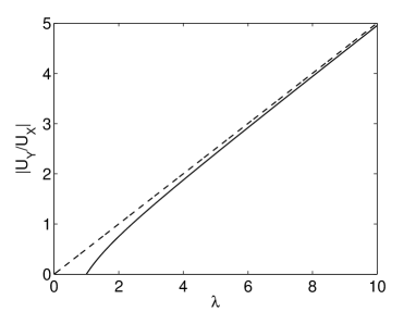
Figure 2: The ratio of velocity components, $|U_{Y}/U_{X}|$, as a function of $\lambda=\sqrt{k_{\|}/k_{\perp}}$.

To maximize $U_{Y}/U_{X}$, $\lambda$ should be as large as possible (Fig. 2), i.e. $k_{\|}$ should be as large, and $k_{\perp}$ should be as small as possible.

Two-component medium.– In order to proceed further, the analysis is now restricted to a two-component anisotropic medium with permeabilities $k_{1},k_{2}$. Consider without loss of generality that $0\leq k_{1}<k_{2}<\infty$. The largest possible $k_{\|}$ corresponds to the upper Wiener bound Torquato (2002):

$$k_{\|}=\phi_{1}k_{1}+\phi_{2}k_{2},$$

where $\phi_{1}$ and $\phi_{2}$ are the area fractions of the two phases with $\phi_{1}+\phi_{2}=1$. The smallest possible $k_{\perp}$ corresponds to the lower Wiener bound:

$$k_{\perp}=\left(\frac{\phi_{1}}{k_{1}}+\frac{\phi_{2}}{k_{2}}\right)^{-1}$$

A texture satisfying simultaneously both conditions exists: it is a configuration of stripes.

We then have for this texture

$$\lambda^{2}=\frac{k_{\|}}{k_{\perp}}=1+\phi_{1}(1-\phi_{1})\frac{(k_{1}-k_{2})^{2}}{k_{1}k_{2}}$$

The surface fraction $\phi_{1}$ corresponding to a maximum of $U_{Y}/U_{X}$ can be found from the equation

$$\frac{\partial}{\partial\phi_{1}}\left|\frac{U_{Y}}{U_{X}}\right|=\frac{1}{2}\left(1+\frac{1}{\lambda^{2}}\right)\frac{1}{2\lambda}\frac{\partial\lambda^{2}}{\partial\phi_{1}}$$

which leads to $\partial\lambda^{2}/\partial\phi_{1}=0$, which is satisfied at $\phi_{1}=1/2$. This extremum corresponds to a maximum and then

$$\lambda^{2}=1+\frac{(k_{1}-k_{2})^{2}}{4k_{1}k_{2}}=\frac{(k_{1}+k_{2})^{2}}{4k_{1}k_{2}}$$

Defining:

$$\overline{k}=\frac{k_{1}+k_{2}}{2},\,\,\,\langle k\rangle=\sqrt{k_{1}k_{2}},$$

the maximum occurs at:

$$\lambda=\frac{\overline{k}}{\langle k\rangle}$$ (5)

and its value is:

$$\left|\frac{U_{Y}}{U_{X}}\right| = \frac{1}{2}\left(\frac{\overline{k}}{\langle k\rangle}-\frac{\langle k\rangle}{\overline{k}}\right)$$ (6)

$$= \frac{1}{2}\left[\frac{1+k_{2}/k_{1}}{2\sqrt{k_{2}/k_{1}}}-\frac{2\sqrt{k_{2}/k_{1}}}{1+k_{2}/k_{1}}.\right]$$

which increases monotonously with the anisotropy, $k_{2}/k_{1}$. It is interesting to note that the preceding analysis applies to any incompressible, gradient-driven “flow” in a two-component medium, not only fluid flow, but also electrical conduction (in which case, we have maximized the transverse current).

Superhydrophobic channels.– We now apply these results to transverse viscous flow in textured, slipping microchannels. We focus first on rough hydrophobic surfaces in the Cassie state, where trapped air bubbles Vinogradova et al. (1995); Cottin-Bizonne et al. (2004); Borkent et al. (2007) can lead to dramatic local slip enhancement. To model this, we assume the liquid surface is approximately flat, so the local channel thickness $h=H$ is fixed. This common assumption Lauga and Stone (2003); Cottin-Bizonne et al. (2004) also corresponds to the minimum dissipation Hyväluoma and Harting (2008); Ybert et al. (2007). The liquid contacts the solid only over an area fraction $\phi_{1}$ of the surface with slip length $b_{1}$, while the remaining area fraction $\phi_{2}$ is a free-standing gas-liquid interface. As a simple estimate, lubricating gas sectors of height $\delta$ with viscosity $\mu_{g}$ much smaller than that of the liquid $\mu$ Vinogradova (1995) have a local slip length $b_{2}\approx\delta(\mu/\mu_{g})\approx 50\,\delta$, which can reach tens of $\mu$m. Hydrodynamic slip can also occur at solid hydrophobic sectors Vinogradova (1999); Lauga et al. (2007); Bocquet and Barrat (2007), but with $b_{1}$ less than tens of nm Vinogradova and Yakubov (2003); Vinogradova et al. (2009); Cottin-Bizonne et al. (2005).

We now consider two cases Feuillebois et al. (2009): (I) one slip wall ($\beta^{+}=\beta;\beta^{-}=0$), and (II) equal slip on opposite surfaces ($\beta^{+}=\beta^{-}=\beta$). Case (I) is relevant for various setups where the alignment of opposite textures is inconvenient or difficult. Case (II) is normally used to minimize the drag Feuillebois et al. (2009). In each case, we have a two-component medium where $\beta$ is either $\beta_{1}$ or $\beta_{2}$. The permeability can now be expressed in term of the gap and slip lengths, Eq. (2). Then, for $j=1,2$:

$$k_{j}=\begin{cases}1+3\beta_{j}/[1+\beta_{j}]&\mbox{ case (I)}\\ 1+6\beta_{j}&\mbox{ case (II)}\end{cases}$$ (7)

Since $h$ is constant, the largest $k_{2}/k_{1}$ obviously corresponds to a largest physically possible $\beta_{2}$ with smallest possible $\beta_{1}$, that is $\beta_{1}=0$.

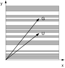
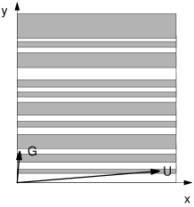
Figure 3: Results of transverse flow optimization for flat microchannels with one superhydrophobic and one no-slip wall (case I, left) and two aligned superhydrophobic walls (case II, right). In both cases, the thickness of stripes is taken as random, to emphasize that the design does not have to be periodic. The mean surface fraction of each component is 1/2. As an example, the distribution of thicknesses is Gaussian with a standard deviation of 0.2. For case II, $\beta_{2}=100$, and $U_{x}\simeq 300G$ has been shortened for visibility.

In case (I), approximating the largest possible $\beta_{2}$ by $\beta_{2}\to\infty$ gives $k_{2}/k_{1}=4$. We obtain $\lambda=\overline{k}/\langle k\rangle=5/4$. The direction of G is $\alpha=\arctan(5/4)=51.34^{\circ}$. Then $|U_{Y}/U_{X}|\to 9/40=0.225$. The direction of U is $\alpha+\theta=\arctan(5/4)-\arctan(9/40)=38.66^{\circ}$ (see Fig. 3a), corresponding to a maximum deflection of almost $13^{\circ}$.

In case (II), the deflection can be more dramatic, but the analysis is more subtle. For $\beta_{2}\gg 1$, $k_{2}\simeq 6\beta_{2}$, the angle $\alpha$ is close to $\pi/2$. Depending on which of the two limits $\beta_{2}\to\infty$ and $\alpha\to\pi/2$ is taken first, the results are different. The resolution of this singular perturbation problem is to find the significant degeneracy Eckhaus (1979), that is the most general limit from which all other cases may be obtained. It can be proved here that the significant degeneracy is obtained for our optimum. We then calculate the following first order approximation:

$$\alpha\simeq\frac{\pi}{2}-\sqrt{\frac{2(1+6\beta_{1})}{3\beta_{2}}},$$

$$U_{X}\simeq 4G(1+6\beta_{1}),\quad U_{Y}\simeq-\sqrt{6\beta_{2}(1+6\beta_{1})}\,G.$$

The angle of U and G is then $\theta\simeq\pi/2-2\sqrt{2(1+6\beta_{1})/3\beta_{2}}$. Note that the flow in this direction close to $\alpha=\pi/2$ is large, but is yet $O(\sqrt{\beta_{2}})$ smaller than the flow that would exist in the $X$ direction for $\alpha=0$.

For completeness, we also apply our results to the Wenzel state, where the liquid is assumed to follow all the topological variations of the material. This leads to a variable thickness for the liquid domain, but fixed hydrodynamic boundary condition. Therefore, the slip length $\beta$ is fixed (possibly zero), but channel thickness $h$ may take two values, $H_{1}$ and $H_{2}$ ($H_{2}>H_{1}$). It is now convenient to define $H_{1}=H$ on the top of asperities, as we defined for the Cassie case. It is easy then to show that $k_{2}/k_{1}=(H_{2}/H)^{2}$. Replacing this value in (6) shows that $H_{2}/H$ should be as large as possible. This limit is very different from the small surface height modulations and lubrication geometries considered by Stroock et al Stroock et al. (2002b) and suggests that further improvements in passive chaotic mixers may be possible with deeper grooves and thinner channels.

Concluding remarks.– A striking conclusion from our analysis is that the surface textures which optimize transverse flow can significantly differ from those optimizing effective (forward) slip. It is well known that the effective slip of a superhydrophobic surface is maximized by reducing the solid-liquid area fraction $\phi_{1}$ Ybert et al. (2007); Feuillebois et al. (2009), until the Cassie state becomes metastable Quere (2008). In contrast, we have shown that transverse flow in thin channels is maximized by stripes with a rather large solid fraction, $\phi_{1}=1/2$, where the Cassie state is typically stable. In this situation, the effective slip $\beta^{*}$ is relatively small Feuillebois et al. (2009), and yet the flow deflection is very strong (nearly $\pi/2$).

These results may guide the design of superhydrophobic surfaces for robust transverse flows in microfluidic devices. Applications may include flow detection, droplet or particle sorting, or passive mixing. The latter results from interactions with side walls, which produce transverse vortices (due to pressure-driven backflow) and overall helical streamlines, which can be made chaotic for efficient mixing by modulating the surface texture in the axial direction, e.g. with herringbone patterns Stroock et al. (2002b, a); Stroock and McGraw (2004); Villermaux et al. (2008). Compared to the grooved no-slip surfaces with small height variations used in prior work, we have shown that slipping (Cassie) and highly rough (Wenzel) surfaces can exhibit much stronger flow deflection in thin channels, which could lead to more efficient mixing upon spatial modulation of the texture.

Another fruitful direction could be to consider transverse electrokinetic phenomena Ajdari (2001), e.g. for flow sensors or electro-osmotic pumps Gitlin et al. (2003). It was recently shown that flat superhydrophobic surfaces can exhibit tensorial electro-osmotic mobility Bahga et al. (2010): Anisotropy is maximized if the Debye screening length $\lambda_{D}$ is comparable to the texture scale, and the gas-liquid interface is uncharged (which, again, does not maximize forward flow); the electro-osmotic mobility scales as, ${\bf M_{e}}\propto({\bf I}+{\bf b}/\lambda_{D})$ in the limit of thick double layers and even thicker channels ($L\ll\lambda_{D}\ll H$) Bahga et al. (2010). If a similar relation holds for thin channels ($H\ll L\ll\lambda_{D}$), then our results for the effective ${\bf b}$ (from ${\bf k}$ in case II Feuillebois et al. (2009)) suggest that transverse electrokinetic phenomena could be greatly amplified by using striped superhydrophobic surfaces.

This research was partly supported by the DFG under the Priority programme “Micro and nanofluidics” (grant Vi 243/1-3).

References

- Quere (2005) D. Quere, Rep. Prog. Phys. 68, 2495 (2005).
- Stone et al. (2004) H. A. Stone, A. D. Stroock, and A. Ajdari, Annual Review of Fluid Mechanics 36, 381 (2004).
- Squires and Quake (2005) T. M. Squires and S. R. Quake, Rev. Mod. Phys. 77, 977 (2005).
- Ybert et al. (2007) C. Ybert, C. Barentin, C. Cottin-Bizonne, P. Joseph, and L. Bocquet, Phys. Fluids 19, 123601 (2007).
- Feuillebois et al. (2009) F. Feuillebois, M. Z. Bazant, and O. I. Vinogradova, Phys. Rev. Lett. 102, 026001 (2009).
- Vinogradova et al. (2009) O. I. Vinogradova, K. Koynov, A. Best, and F. Feuillebois, Phys. Rev. Lett. 102, 118302 (2009).
- Vinogradova and Yakubov (2003) O. I. Vinogradova and G. E. Yakubov, Langmuir 19, 1227 (2003).
- Cottin-Bizonne et al. (2005) C. Cottin-Bizonne, B. Cross, A. Steinberger, and E. Charlaix, Phys. Rev. Lett. 94, 056102 (2005).
- Squires (2008) T. M. Squires, Phys. Fluids 20, 092105 (2008).
- Bahga et al. (2010) S. S. Bahga, O. I. Vinogradova, and M. Z. Bazant, J. Fluid Mech. 644, 245 (2010).
- Huang et al. (2008) D. M. Huang, C. Cottin-Bizonne, C. Ybert, and L. Bocquet, Phys. Rev. Lett. 20, 092105 (2008).
- Quere (2008) D. Quere, Annu. Rev. Mater. Res. 38, 71 (2008).
- Bazant and Vinogradova (2008) M. Z. Bazant and O. I. Vinogradova, J. Fluid Mech. 613, 125 (2008).
- Kamrin et al. (2010) K. Kamrin, M. Z. Bazant, and H. A. Stone, J. Fluid Mech. in press (2010).
- Ajdari (2001) A. Ajdari, Phys. Rev. E 65, 016301 (2001).
- Stroock et al. (2002a) A. D. Stroock, S. K. W. Dertinger, A. Ajdari, I. Mezić, H. A. Stone, and G. M. Whitesides, Science 295, 647 (2002a).
- Wang (2003) C. Y. Wang, Physics of Fluids 15, 1114 (2003).
- Stroock et al. (2002b) A. D. Stroock, S. K. Dertinger, G. M. Whitesides, and A. Ajdari, Anal. Chem. 74, 5306 (2002b).
- Stroock and McGraw (2004) A. D. Stroock and G. J. McGraw, Philosophical Transactions of the Royal Society A 04TA1803, 1 (2004).
- Villermaux et al. (2008) E. Villermaux, A. D. Stroock, and H. A. Stone, Phys. Rev. E 77, 015301 (2008).
- Torquato (2002) S. Torquato, Random Heterogeneous Materials: Microstructure and Macroscopic Properties (Springer, 2002).
- Vinogradova et al. (1995) O. I. Vinogradova, N. F. Bunkin, N. V. Churaev, O. A. Kiseleva, A. V. Lobeyev, and B. W. Ninham, J. Colloid Interface Sci. 173, 443 (1995).
- Cottin-Bizonne et al. (2004) C. Cottin-Bizonne, C. Barentin, E. Charlaix, L. Bocquet, and J. L. Barrat, Eur. Phys. J. E 15, 427 (2004).
- Borkent et al. (2007) B. M. Borkent, S. M. Dammler, H. Schönherr, G. J. Vansco, and D. Lohse, Phys. Rev. Lett. 98, 204502 (2007).
- Lauga and Stone (2003) E. Lauga and H. A. Stone, J. Fluid Mech. 489, 55 (2003).
- Hyväluoma and Harting (2008) J. Hyväluoma and J. Harting, Phys. Rev. Lett. 100, 246001 (2008).
- Vinogradova (1995) O. I. Vinogradova, Langmuir 11, 2213 (1995).
- Vinogradova (1999) O. I. Vinogradova, Int. J. Mineral Proces. 56, 31 (1999).
- Lauga et al. (2007) E. Lauga, M. P. Brenner, and H. A. Stone, Handbook of Experimental Fluid Dynamics (Springer, NY, 2007), chap. 19, pp. 1219–1240.
- Bocquet and Barrat (2007) L. Bocquet and J. L. Barrat, Soft Matter 3, 685 (2007).
- Eckhaus (1979) W. Eckhaus, Asymptotic analysis of singular perturbations (North-Holland, 1979), studies in Applied Mathematics, vol. 9.
- Gitlin et al. (2003) I. Gitlin, A. D. Stroock, G. M. Whitesides, and A. Ajdari, Appl. Phys. Lett. 83, 1486 (2003).