Spin drag Hall effect in a rotating Bose mixture
Abstract
We show that in a rotating two-component Bose mixture, the spin drag between the two different spin species shows a Hall effect. This spin drag Hall effect can be observed experimentally by studying the out-of-phase dipole mode of the mixture. We determine the damping of this mode due to spin drag as a function of temperature. We find that due to Bose stimulation there is a strong enhancement of the damping for temperatures close to the critical temperature for Bose-Einstein condensation.
pacs:
67.85.-d, 03.75.-b, 05.30.FkIntroduction — Electronic transport is one of the main topics of interest in condensed-matter physics, and an especially important phenomenon in electronic transport is the Hall effect. It was discovered already in the late nineteenth century by Hall. He observed that if a magnetic field is applied perpendicular to the current density through a conductor, the Lorentz force leads to a voltage drop in the direction perpendicular to both the current density and the magnetic field. This voltage is proportional to , with a proportionality constant that depends only on the density of electrons and not on any other material parameters Hall (1879). While the discovery of the Hall effect predates that of the electron, it is important for our purposes to note that electronic transport is in fact fermionic transport since it is mediated by the movement of electrons. By now many variations of the Hall effect have been found: the (integer and fractional) quantum Hall effects in which the Hall voltage is quantized Klitzing et al. (1980); Laughlin (1983); Tsui et al. (1982), the spin Hall effect Murakami et al. (2003); Sinova et al. (2004), and the quantum spin Hall effect Konig et al. (2007). Recently, a spin Hall drag effect has also been proposed Badalyan and Vignale (2009). The latter is, as all spin Hall effects are, due to spin-orbit interactions that play no role in atomic Bose gases if they are not externally introduced by applying an appropriate laser field configuration Stanescu et al. (2008). The proposal of Ref. Badalyan and Vignale (2009) is therefore physically very different from what we discuss below.
An important field of physics which connects few-body atomic physics with many-body and condensed-matter physics is that of cold atoms. The Bose-Einstein condensation of bosons at very low temperatures was already predicted by Einstein in 1924, but only observed directly in 1995 Anderson et al. (1995). Over the past fifteen years, techniques have been getting steadily more refined, and it is now possible to make all sorts of degenerate atomic mixtures consisting of several spin states or of several different atomic species of either fermions or bosons. These mixtures are always trapped in optical and/or magnetic potentials, in which the atoms can be set into rotation by stirring with a so-called laser spoon Madison et al. (2000).
It is tempting to combine the above two fields to also get more insight into the physics of bosonic transport. At first sight this seems less than straightforward, since it is not possible to simply attach leads to a cloud of cold atoms to set up a steady-state transport current of atoms through the mixture. Moreover, in the cold-atom situation there are no obvious mechanisms that relax the particle current and give nonzero resistivities. However, we can use the phenomenon of spin drag as a bridge between these two worlds polini2007 ; Duine and Stoof (2009); Duine et al. (2010). Spin drag was first proposed by D’Amico and Vignale by making an analogy with Coulomb drag between to electron layers D’Amico and Vignale (2000). It was later observed by Weber et al. Weber et al. (2005). Whereas in the classic Coulomb drag experiment electrons are differentiated by the layer they occupy, in spin drag the spin of the electron is the relevant degree of freedom, i.e., electrons of one spin species drag along electrons of the other spin species. The resistivity created by this spin drag, which is a resistivity to spin but not to charge currents, typically goes as in electronic systems, with the temperature. This is the trademark of a Fermi-liquid like behavior.
In our earlier work Duine and Stoof (2009), we investigated the situation in which the particles involved in the spin drag are bosons instead of fermions. We proposed an idealized set-up in which spin-1 bosons in the state are accelerated along a torroidal trap by a time-dependent magnetic-field texture that creates a fictitious electric field. The atoms in state , which are also present, do not feel this force but experience spin drag due to collisions with the other species. We found that due to the Bose enhancement of interatomic scattering, the drag resisitivity increases at lower temperatures. For the one-dimensional set-up considered, it in fact behaves as for low temperatures, in strong contrast with the usual quadratic Fermi-liquid result.
In this Letter, we discuss spin drag in a rotating Bose mixture. We consider the realistic situation of a three-dimensional Bose mixture with two spin components, present in equal numbers, just above the temperature for Bose-Einstein condensation. We first consider the homogeneous case and look in linear response for steady-state solutions of the appropriate Boltzmann equation with a nonzero spin current. We find that the drag resistivity now becomes a matrix with nonzero off-diagonal elements that are proportional to the rotation speed, which represents a Hall effect. Indeed, these off-diagonal elements are analogous to those found in the classical Hall effect and, in particular, do not depend on the specific collisional details of the mixture that determine the diagonal resistivities, but only on the atomic density and external rotation frequency.
As mentioned previously, such steady-state solutions no longer exist in the realistic situation that the atomic mixture is trapped in an external harmonic potential. The spin drag Hall effect can nevertheless be observed in that case by considering the collective modes. In particular, we consider the dipole mode in which the two spin components oscillate out of phase with each other, because this mode obtains an orthogonal, i.e., a transverse component due to the spin drag Hall effect. Moreover, the longitudional spin drag leads to damping of this mode, which makes it interesting to find out how the relaxation rate of these modes depends on temperature. To obtain this, we again solve the Boltzmann equation for this specific case in linear response, and find that the relaxation rate shows a substantial increase as the temperature gets closer to the critical temperature. In three dimensions the relaxation rate does, however, remain finite at the transition temperature.
Spin drag Hall effect— To illustrate the spin drag Hall effect we consider first a homogeneous three-dimensional Bose mixture of two spin states, which we label and , in the normal state. We assume that the bosons in spin state couple to an external force , and that the other spin state does not couple to this external force. (Generalizations to more than two spin species and different forces are straightforward.) This would for example be the case if the external force is due to the Zeeman effect in a magnetic field, and if the two spin states correspond to the and projections of an hyperfine state. We assume that the system is rotating, which gives rise to a Coriolis force that is the equivalent of the the Lorentz force from the electronic Hall effect.
The appropriate Boltzmann equation is
| (1) |
Here, is the distribution function for the bosons in state . The Boltzmann equation for is found by replacing and setting to zero. Furthermore, is the rotation vector, and gives the Coriolis force. The collision term, , describes collisions of atoms with different spin. We will give its precise definition later on. There are of course also collisions between atoms with an identical spin but they do not play a role for the spin drag.
We solve the Boltzmann equation by using the ansatz , with a similar expression for in terms of . Here, is the Bose-Einstein distribution function with , as usual, the inverse thermal energy, Boltzmann’s constant, and the temperature. The single-particle dispersion is with the particle mass. The chemical potential is determined by the condition that the density of atoms is constant. The Boltzmann equation leads to the following equations of motion for the drift velocities and
| (2) | |||||
| (3) |
Here, is the particle density per spin. We assume this density to be equal for the two spin species. Again, note that generalizations of the above to spin and mass imbalanced systems are straightforward.
In general the frictional spin drag is determined by the full nonlinear (vector-valued) function . In the linear-response regime where the velocities are small, we make use of the fact that it can be approximated by . Note that here we make use of the isotropy of the collision term in the Boltzmann equation. We now introduce the relative particle current, which up to dimensionful prefactors is equal to the spin current, and solve the above equations of motion for the steady state, i.e., . We then find that , which defines the conductivity and resistivity tensors and , respectively. Note that these are matrices since the force and current are three-dimensional vectors. We find that the longitudinal resistivities , which are related to the spin drag relaxation time via a Drude-like formula as . This relaxation time is the time scale on which the spin current decays due to collisions of atoms in different spin states. The Hall resistivities are given by . All other components of the resistivity and conductivity tensors are zero. Like the Hall resistivity in electronic systems, the transverse components of the resistivity do not depend on the specifics of the processes that lead to a nonzero longitudinal resistivity, but only on the density and strength of the Coriolis force. The longitudinal resistivity, however, that determines the dissipation of the relative momentum current via frictional spin drag, depends on the inter-spin-species collisions.
Collective modes — To implement the spin drag Hall effect in a realistic cold-atom experiment, we have to take into account the effects of the trapping potential. Steady-state current are now no longer possible. In this situation the collective-mode spectrum of the mixture provides an experimental method to determine the spin drag resistivities. We consider a harmonic trapping potential with radial trapping frequency and axial frequency . We now have for the Boltzmann equation
| (4) |
where includes the centrifugal force. The equation for is again found by replacing .
We solve this inhomogeneous Boltzmann equation by making the ansatz , with a similar expression for . This ansatz is now parameterized by the center-of-mass velocities and positions of the two atomic clouds. From this, we get the equations of motion.
| (5) | |||
| (6) |
with the particle number per spin state. Note that due to the centrifugal force, we need to have that .
We again linearize the above equations using that due to the isotropy of the collision integral. We next observe that all the motion in the -direction decouples. We therefore only consider the motion of the clouds in the -plane, since this contains the spin drag Hall effect. The linearized equations then yield a collective-mode spectrum with eight modes in total. There are four modes in which the two clouds of particles move in phase, and in which there is, as a result, no drag effect. The modes correspond physically to in-phase harmonic oscillations of the two clouds with frequencies . There are two different frequencies because the degeneracy due to the two equivalent directions of oscillation in the effective two-dimensional system, is split by the external rotation. The four out-of-phase modes correspond physically to the two atomic clouds moving relative to each other. This results in transfer of momentum between the two clouds, leading to spin drag and damping of these modes. These modes have the frequencies
| (7) |
The imaginary part of the above frequencies gives the damping rate of the modes, and is for given by with the spin drag relaxation time. This relaxation time gives the longitudinal spin drag resistivity as , and is estimated next. From the eigenvectors of the modes we find that the plane of oscillation of the out-of-phase dipole mode is not fixed in the co-rotating frame, which implies a transverse spin current. This is the trap equivalent of the spin drag Hall effect discussed in the previous section.
Spin drag relaxation time — In the inhomogeneous case, we find that
| (8) |
where
Here, is the two-body T-matrix, which equals , with the scattering length for inter-spin-species collisions. Introducing the response function
| (9) | |||
we find
| (10) | |||||
from which we can determine the spin drag relaxation time. The imaginary part of the response function is worked out explicitly to yield
| (11) | |||
with the thermal de Broglie wavelength and .
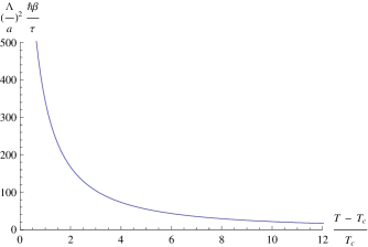
We estimate the above expression for a three-dimensional homogeneous system with density for which we, in first approximation, have take the central density in the trap to make connection with the inhomogeneous case. The result for is evaluated numerically, and is shown in Fig. 1. We see that Bose enhancement is indeed at play: gets dramatically bigger as the temperature approaches the critical temperature. We do find, however, that it remains finite as . Furthermore, from our numerical results, we find that .
Discussion and conclusion— We have introduced the spin drag Hall effect, i.e., the emergence of a transverse spin current, in rotating Bose mixtures. To determine whether the spin drag relaxation rate can be measured in principle, we make estimates of the relaxation time for some realistic values of the parameters. Taking for instance 87Rb at temperatures between 10 and 100 nK, with an inter-species scattering length of about 100 Bohr radii, we find values of the order of ms for densities cm-3. Considering that the trapping potential usually has kHz, this means the damping should indeed happen on an observable time scale. To compare with electronic systems we note that the Drude formula (with the electronic charge to convert to units of electrical resistivity) with our result for yields resistivities of the order of m, many orders of magnitude larger than the spin drag resistivity in an electronic system Polini and Vignale (2009).
One interesting aspect of the Bose enhancement of the is the behavior close to the critical temperature. Here, we numerically found that , with within our numerical accuracy. In future work we intend to investigate the value of this exponent in various dimensions with renormalization-group methods, taking into account critical fluctuations that are not captured by the Boltzmann approach presented here. Note that in our previous work concerning one spatial dimension, we found a divergence of the spin drag relaxation rate as Duine and Stoof (2009), also with Boltzmann methods. An interesting aspect of a two-component Bose mixture is that it also may become ferromagnetic above the critical temperature of Bose-Einstein condensation. We intend to study also the effects of this transition on the spin drag.
The collective mode spectrum determined theoretically in this Letter can be observed experimentally by setting the two spin states in relative motion. This can for example be achieved by shortly applying small magnetic field gradient to excite the spin-dipole mode. Another possibility is to use a state-selective laser in a manner that is similar to the generation of the second-sound dipole mode in a partially Bose-Einstein condensed gas Meppelink et al. (2009).
We hope that the close collaboration between theory and experiments in this area, will lead to more insight into bosonic transport and, on the long run, may eventually lead to the development of useful atomtronics devices pepino2009 , where atoms rather than electrons are the main carriers of transport.
This work was supported by the Stichting voor Fundamenteel Onderzoek der Materie (FOM), the Netherlands Organization for Scientific Research (NWO), and by the European Research Council (ERC) under the Seventh Framework Program (FP7).
References
- Hall (1879) E. H. Hall, American Journal of Mathematics 2, 287 (1879).
- Klitzing et al. (1980) K. v. Klitzing, G. Dorda, and M. Pepper, Phys. Rev. Lett. 45, 494 (1980).
- Laughlin (1983) R. B. Laughlin, Phys. Rev. Lett. 50, 1395 (1983).
- Tsui et al. (1982) D. C. Tsui, H. L. Stormer, and A. C. Gossard, Phys. Rev. Lett. 48, 1559 (1982).
- Murakami et al. (2003) S. Murakami, N. Nagaosa, and S.-C. Zhang, Science 301, 1348 (2003).
- Sinova et al. (2004) J. Sinova, D. Culcer, Q. Niu, N. A. Sinitsyn, T. Jungwirth, and A. H. MacDonald, Phys. Rev. Lett. 92, 126603 (2004).
- Konig et al. (2007) M. Konig, S. Wiedmann, C. Brune, A. Roth, H. Buhmann, L. W. Molenkamp, X.-L. Qi, and S.-C. Zhang, Science p. 1148047 (2007).
- Badalyan and Vignale (2009) S. M. Badalyan and G. Vignale, Phys. Rev. Lett. 103, 196601 (2009).
- Stanescu et al. (2008) T. D. Stanescu, B. Anderson, and V. Galitski, Phys. Rev. A 78, 023616 (2008).
- Anderson et al. (1995) M. H. Anderson, J. R. Ensher, M. R. Matthews, C. E. Wieman, and E. A. Cornell, Science 269, 198 (1995).
- Madison et al. (2000) K. W. Madison, F. Chevy, W. Wohlleben, and J. Dalibard, Phys. Rev. Lett. 84, 806 (2000).
- (12) M. Polini, and G. Vignale, Phys. Rev. Lett. 98, 266403 (2007).
- Duine and Stoof (2009) R. A. Duine and H. T. C. Stoof, Phys. Rev. Lett. 103, 170401 (2009).
- Duine et al. (2010) R. A. Duine, M. Polini, H. T. C. Stoof, and G. Vignale, Phys. Rev. Lett. 104, 220403 (2010).
- D’Amico and Vignale (2000) I. D’Amico and G. Vignale, Phys. Rev. B 62, 4853 (2000).
- Weber et al. (2005) C. Weber, N. Gedik, J. Moore, J. Orenstein, J. Stephens, and D. Awschalom, Nature 437, 1330 (2005).
- Polini and Vignale (2009) M. Polini and G. Vignale, Physics 2, 87 (2009).
- Meppelink et al. (2009) R. Meppelink, S. B. Koller, J. M. Vogels, H. T. C. Stoof, and P. van der Straten, Phys. Rev. Lett. 103, 265301 (2009).
- (19) R. A. Pepino, J. Cooper, D. Z. Anderson, and M. J. Holland, Phys. Rev. Lett. 103, 140405 (2009).