Abstract

A popular method for selecting the number of clusters is based on stability arguments: one chooses the number of clusters such that the corresponding clustering results are “most stable”. In recent years, a series of papers has analyzed the behavior of this method from a theoretical point of view. However, the results are very technical and difficult to interpret for non-experts. In this paper we give a high-level overview about the existing literature on clustering stability. In addition to presenting the results in a slightly informal but accessible way, we relate them to each other and discuss their different implications.

Chapter 0 Introduction

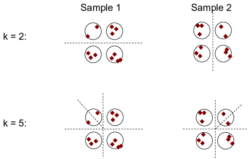
Figure 1: Idea of clustering stability. Instable clustering solutions if the number of clusters is too small (first row) or too large (second row). See text for details.

Model selection is a difficult problem in non-parametric clustering. The obvious reason is that, as opposed to supervised classification, there is no ground truth against which we could “test” our clustering results. One of the most pressing questions in practice is how to determine the number of clusters. Various ad-hoc methods have been suggested in the literature, but none of them is entirely convincing. These methods usually suffer from the fact that they implicitly have to define “what a clustering is” before they can assign different scores to different numbers of clusters. In recent years a new method has become increasingly popular: selecting the number of clusters based on clustering stability. Instead of defining “what is a clustering”, the basic philosophy is simply that a clustering should be a structure on the data set that is “stable”. That is, if applied to several data sets from the same underlying model or of the same data generating process, a clustering algorithm should obtain similar results. In this philosophy it is not so important how the clusters look (this is taken care of by the clustering algorithm), but that they can be constructed in a stable manner.

The basic intuition of why people believe that this is a good principle can be described by Figure 1. Shown is a data distribution with four underlying clusters (depicted by the black circles), and different samples from this distribution (depicted by red diamonds). If we cluster this data set into $K=2$ clusters, there are two reasonable solutions: a horizontal and a vertical split. If a clustering algorithm is applied repeatedly to different samples from this distribution, it might sometimes construct the horizontal and sometimes the vertical solution. Obviously, these two solutions are very different from each other, hence the clustering results are instable. Similar effects take place if we start with $K=5$. In this case, we necessarily have to split an existing cluster into two clusters, and depending on the sample this could happen to any of the four clusters. Again the clustering solution is instable. Finally, if we apply the algorithm with the correct number $K=4$, we observe stable results (not shown in the figure): the clustering algorithm always discovers the correct clusters (maybe up to a few outlier points). In this example, the stability principle detects the correct number of clusters.

At first glance, using stability-based principles for model selection appears to be very attractive. It is elegant as it avoids to define what a good clustering is. It is a meta-principle that can be applied to any basic clustering algorithm and does not require a particular clustering model. Finally, it sounds “very fundamental” from a philosophy of inference point of view.

However, the longer one thinks about this principle, the less obvious it becomes that model selection based on clustering stability “always works”. What is clear is that solutions that are completely instable should not be considered at all. However, if there are several stable solutions, is it always the best choice to select the one corresponding to the most stable results? One could conjecture that the most stable parameter always corresponds to the simplest solution, but clearly there exist situations where the most simple solution is not what we are looking for. To find out how model selection based on clustering stability works we need theoretical results.

In this paper we discuss a series of theoretical results on clustering stability that have been obtained in recent years. In Section 1 we review different protocols for how clustering stability is computed and used for model selection. In Section 2 we concentrate on theoretical results for the $K$-means algorithm and discuss their various relations. This is the main section of the paper. Results for more general clustering algorithms are presented in Section 3.

Chapter 1 Clustering stability: definition and implementation

A clustering of a data set $S=\{X_{1},\ldots,X_{n}\}$ is a function that assigns labels to all points of $S$, that is $\mathcal{C}_{K}:S\to\{1,\ldots,K\}.$ Here $K$ denotes the number of clusters. A clustering algorithm is a procedure that takes a set $S$ of points as input and outputs a clustering of $S$. The clustering algorithms considered in this paper take an additional parameter as input, namely the number $K$ of clusters they are supposed to construct.

We analyze clustering stability in a statistical setup. The data set $S$ is assumed to consist of $n$ data points $X_{1},\ldots,X_{n}$ that have been drawn independently from some unknown underlying distribution $P$ on some space $\mathcal{X}$. The final goal is to use these sample points to construct a good partition of the underlying space $\mathcal{X}$. For some theoretical results it will be easier to ignore sampling effects and directly work on the underlying space $\mathcal{X}$ endowed with the probability distribution $P$. This can be considered as the case of having “infinitely many” data points. We sometimes call this the limit case for $n\to\infty$.

Assume we agree on a way to compute distances $d(\mathcal{C},\mathcal{C}^{\prime})$ between different clusterings $\mathcal{C}$ and $\mathcal{C}^{\prime}$ (see below for details). Then, for a fixed probability distribution $P$, a fixed number $K$ of clusters and a fixed sample size $n$, the instability of a clustering algorithm is defined as the expected distance between two clusterings $\mathcal{C}_{K}(S_{n})$, $\mathcal{C}_{K}(S_{n}^{\prime})$ on different data sets $S_{n}$, $S_{n}^{\prime}$ of size $n$, that is

$$\operatorname{Instab}(K,n):=E\big{(}\;d(\mathcal{C}_{K}(S_{n}),\mathcal{C}_{K}(S_{n}^{\prime}))\;\big{)}$$ (1)

The expectation is taken with respect to the drawing of the two samples.

In practice, a large variety of methods has been devised to compute stability scores and use them for model selection. On a very general level they works as follows:

• Given: a set $S$ of data points, a clustering algorithm $\mathcal{A}$ that takes the number $k$ of clusters as input

  1. For $k=2,\ldots,k_{\max}$

     1. Generate perturbed versions $S_{b}$ $(b=1,\ldots,b_{\max})$ of the original data set (for example by subsampling or adding noise, see below)

     2. For $b=1,\ldots,b_{\max}$:
        Cluster the data set $S_{b}$ with algorithm $\mathcal{A}$ into $k$ clusters to obtain clustering $\mathcal{C}_{b}$

     3. For $b,b^{\prime}=1,\ldots,b_{\max}$:
        Compute pairwise distances $d(\mathcal{C}_{b},\mathcal{C}_{b^{\prime}})$ between these clusterings (using one of the distance functions described below)

     4. Compute instability as the mean distance between clusterings $\mathcal{C}_{b}$:

        $$\widehat{\operatorname{Instab}}(k,n)=\frac{1}{b_{\max}^{2}}\sum_{b,b^{\prime}=1}^{b_{max}}\;d(\mathcal{C}_{b},\mathcal{C}_{b^{\prime}})$$

  2. Choose the parameter $k$ that gives the best stability, in the simplest case as follows:

     $$K:=\operatorname*{argmin}_{k}\widehat{\operatorname{Instab}}(k,n)$$

     (see below for more options).

This scheme gives a very rough overview of how clustering stability can be used for model selection. In practice, many details have to be taken into account, and they will be discussed in the next section. Finally, we want to mention an approach that is vaguely related to clustering stability, namely the ensemble method (Strehl and Ghosh, 2002). Here, an ensemble of algorithms is applied to one fixed data set. Then a final clustering is built from the results of the individual algorithms. We are not going to discuss this approach in our paper.

Generating perturbed versions of the data set. To be able to evaluate the stability of a fixed clustering algorithm we need to run the clustering algorithm several times on slightly different data sets. To this end we need to generate perturbed versions of the original data set. In practice, the following schemes have been used:

• Draw a random subsample of the original data set without replacement (Levine and Domany, 2001, Ben-Hur et al., 2002, Fridlyand and Dudoit, 2001, Lange et al., 2004).
  

• Add random noise to the original data points (Bittner et al., 2000, Möller and Radke, 2006).
  

• If the original data set is high-dimensional, use different random projections in low-dimensional spaces, and then cluster the low-dimensional data sets (Smolkin and Ghosh, 2003).
  

• If we work in a model-based framework, sample data from the model (Kerr and Churchill, 2001).
  

• Draw a random sample of the original data with replacement. This approach has not been reported in the literature yet, but it avoids the problem of setting the size of the subsample. For good reasons, this kind of sampling is the standard in the bootstrap literature (Efron and Tibshirani, 1993) and might also have advantages in the stability setting. This scheme requires that the algorithm can deal with weighted data points (because some data points will occur several times in the sample).
  

In all cases, there is a trade-off that has to be treated carefully. If we change the data set too much (for example, the subsample is too small, or the noise too large), then we might destroy the structure we want to discover by clustering. If we change the data set too little, then the clustering algorithm will always obtain the same results, and we will observe trivial stability. It is hard to quantify this trade-off in practice.

Which clusterings to compare? Different protocols are used to compare the clusterings on the different data sets $S_{b}$.

• Compare the clustering of the original data set with the clusterings obtained on subsamples (Levine and Domany, 2001).
  

• Compare clusterings of overlapping subsamples on the data points where both clusterings are defined. (Ben-Hur et al., 2002).
  

• Compare clusterings of disjoint subsamples (Fridlyand and Dudoit, 2001, Lange et al., 2004). Here we first need to apply an extension operator to extend each clustering to the domain of the other clustering.
  

Distances between clusterings. If two clusterings are defined on the same data points, then it is straightforward to compute a distance score between these clusterings based on any of the well-known clustering distances such as the Rand index, Jaccard index, Hamming distance, minimal matching distance, Variation of Information distance (Meila, 2003). All these distances count, in some way or the other, points or pairs of points on which the two clusterings agree or disagree. The most convenient choice from a theoretical point of view is the minimal matching distance. For two clusterings $\mathcal{C},\mathcal{C}^{\prime}$ of the same data set of $n$ points it is defined as

$$d_{\text{MM}}(\mathcal{C},\mathcal{C}^{\prime}):=\min_{\pi}\frac{1}{n}\sum_{i=1}^{n}\mathbb{1}_{\{\mathcal{C}(X_{i})\neq\pi(\mathcal{C}^{\prime}(X_{i}))\}}$$ (2)

where the minimum is taken over all permutations $\pi$ of the $K$ labels. Intuitively, the minimal matching distance measures the same quantity as the 0-1-loss used in supervised classification. For a stability study involving the adjusted Rand index or an adjusted mutual information index see Vinh and Epps (2009).

If two clusterings are defined on different data sets one has two choices. If the two data sets have a big overlap one can use a restriction operator to restrict the clusterings to the points that are contained in both data sets. On this restricted set one can then compute a standard distance between the two clusterings. The other possibility is to use an extension operator to extend both clusterings from their domain to the domain of the other clustering. Then one can compute a standard distance between the two clusterings as they are now both defined on the joint domain. For center-based clusterings, as constructed by the $K$-means algorithm, a natural extension operator exists. Namely, to a new data point we simply assign the label of the closest cluster center. A more general scheme to extend an existing clustering to new data points is to train a classifier on the old data points and use its predictions as labels on the new data points. However, in the context of clustering stability it is not obvious what kind of bias we introduce with this approach.

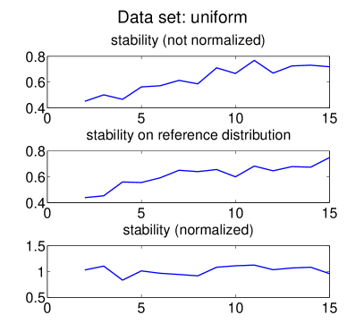
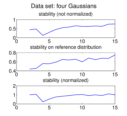
Figure 1: Normalized stability scores. Left plots: data points from a uniform density on $[0,1]^{2}$. Right plots: data points from a mixture of four well-separated Gaussians in $\mathbb{R}^{2}$. The first row always shows the unnormalized instability $\widehat{\operatorname{Instab}}$ for $K=2,...,15$. The second row shows the instability $\widehat{\operatorname{Instab}}_{\text{norm}}$ obtained on a reference distribution (uniform distribution). The third row shows the normalized stability $\widehat{\operatorname{Instab}}_{\text{norm}}$.

Stability scores and their normalization. The stability protocol outlined above results in a set of distance values $(d(\mathcal{C}_{b},\mathcal{C}_{b^{\prime}}))_{b,b^{\prime}=1,\ldots,b_{max}}$. In most approaches, one summarizes these values by taking their mean:

$$\widehat{\operatorname{Instab}}(k,n)=\frac{1}{b_{\max}^{2}}\sum_{b,b^{\prime}=1}^{b_{max}}\;d(\mathcal{C}_{b},\mathcal{C}_{b^{\prime}})$$

Note that the mean is the simplest summary statistic one can compute based on the distance values $d(\mathcal{C}_{b},\mathcal{C}_{b^{\prime}})$. A different approach is to use the area under the cumulative distribution function of the distance values as the stability score, see Ben-Hur et al. (2002) or Bertoni and Valentini (2007) for details. In principle one could also come up with more elaborate statistics based on distance values. To the best of our knowledge, such concepts have not been used so far.

The simplest way to select the number $K$ of clusters is to minimize the instability:

$$K=\operatorname*{argmin}_{k=2,\ldots,k_{\max}}\widehat{\operatorname{Instab}}(k,n).$$

This approach has been suggested in Levine and Domany (2001). However, an important fact to note is that $\widehat{\operatorname{Instab}}(k,n)$ trivially scales with $k$, regardless of what the underlying data structure is. For example, in the top left plot in Figure 1 we can see that even for a completely unclustered data set, $\widehat{\operatorname{Instab}}(n,k)$ increases with $k$. When using stability for model selection, one should correct for the trivial scaling of $\widehat{\operatorname{Instab}}$, otherwise it might be meaningless to take the minimum afterwards. There exist several different normalization protocols:

• Normalization using a reference null distribution (Fridlyand and Dudoit, 2001, Bertoni and Valentini, 2007). One repeatedly samples data sets from some reference null distribution. Such a distribution is defined on the same domain as the data points, but does not possess any cluster structure. In simple cases one can use the uniform distribution on the data domain as null distribution. A more practical approach is to scramble the individual dimensions of the existing data points and use the “scrambled points” as null distribution (see Fridlyand and Dudoit, 2001, Bertoni and Valentini, 2007 for details). Once we have drawn several data sets from the null distribution, we cluster them using our clustering algorithm and compute the corresponding stability score $\widehat{\operatorname{Instab}}_{\text{null}}$ as above. The normalized stability is then defined as $\widehat{\operatorname{Instab}}_{\text{norm}}:=\widehat{\operatorname{Instab}}/\widehat{\operatorname{Instab}}_{\text{null}}$.
  

• Normalization by random labels (Lange et al., 2004). First, we cluster each of the data sets $S_{b}$ as in the protocol above to obtain the clusterings $\mathcal{C}_{b}$. Then, we randomly permute these labels. That is, we assign the label to data point $X_{i}$ that belonged to $X_{\pi(i)}$, where $\pi$ is a permutation of $\{1,\ldots,n\}$. This leads to a permuted clustering $\mathcal{C}_{b,\text{ perm}}$. We then compute the stability score $\widehat{\operatorname{Instab}}$ as above, and similarly we compute $\widehat{\operatorname{Instab}}_{\text{perm}}$ for the permuted clusterings. The normalized stability is then defined as $\widehat{\operatorname{Instab}}_{\text{norm}}:=\widehat{\operatorname{Instab}}/\widehat{\operatorname{Instab}}_{\text{perm}}$.
  

Once we computed the normalized stability scores $\widehat{\operatorname{Instab}}_{\text{norm}}$ we can choose the number of clusters that has smallest normalized instability, that is

$$K=\operatorname*{argmin}_{k=2,\ldots,k_{\max}}\widehat{\operatorname{Instab}}_{\text{norm}}(k,n)$$

This approach has been taken for example in Ben-Hur et al. (2002), Lange et al. (2004).

Selecting $K$ based on statistical tests. A second approach to select the final number of clusters is to use a statistical test. Similarly to the normalization considered above, the idea is to compute stability scores not only on the actual data set, but also on “null data sets” drawn from some reference null distribution. Then one tests whether, for a given parameter $k$, the stability on the actual data is significantly larger than the one computed on the null data. If there are several values $k$ for which this is the case, then one selects the one that is most significant. The most well-known implementation of such a procedure uses bootstrap methods (Fridlyand and Dudoit, 2001). Other authors use a $\chi^{2}$-test (Bertoni and Valentini, 2007) or a test based on the Bernstein inequality (Bertoni and Valentini, 2008).

To summarize, there are many different implementations for selecting the number $K$ of clusters based on stability scores. Until now, there does not exist any convincing empirical study that thoroughly compares all these approaches on a variety of data sets. In my opinion, even fundamental issues such as the normalization have not been investigated in enough detail. For example, in my experience normalization often has no effect whatsoever (but I did not conduct a thorough study either). To put stability-based model selection on a firm ground it would be crucial to compare the different approaches with each other in an extensive case study.

Chapter 2 Stability analysis of the $K$-means algorithm

The vast majority of papers about clustering stability use the $K$-means algorithm as basic clustering algorithm. In this section we discuss the stability results for the $K$-means algorithm in depth. Later, in Section 3 we will see how these results can be extended to other clustering algorithms.

For simpler reference we briefly recapitulate the $K$-means algorithm (details can be found in many text books, for example Hastie et al., 2001). Given a set of $n$ data points $X_{1},\ldots,X_{n}\in\mathbb{R}^{d}$ and a fixed number $K$ of clusters to construct, the $K$-means algorithm attempts to minimize the clustering objective function

$$Q^{(n)}_{K}(c_{1},\ldots,c_{K})=\frac{1}{n}\sum_{i=1}^{n}\min_{k=1,..,K}\|X_{i}-\text{c}_{k}\|^{2}$$ (1)

where $c_{1},\ldots,c_{K}$ denote the centers of the $K$ clusters. In the limit $n\to\infty$, the $K$-means clustering is the one that minimizes the limit objective function

$$Q^{(\infty)}_{K}(c_{1},\ldots,c_{K})=\int\min_{k=1,..,K}\|X-\text{c}_{k}\|^{2}\;dP(X)$$ (2)

where $P$ is the underlying probability distribution.

Given an initial set $c^{<0>}=\{c_{1}^{<0>},\ldots,c_{K}^{<0>}\}$ of centers, the $K$-means algorithm iterates the following two steps until convergence:

• 1. Assign data points to closest cluster centers:

     $$\forall i=1,\ldots,n:\;\;\;\mathcal{C}^{<t>}(X_{i}):=\operatorname*{argmin}_{k=1,\ldots K}\|X_{i}-c_{k}^{<t>}\|$$

  2. Re-adjust cluster means:

     $$\forall k=1,\ldots,K:\;\;\;c_{k}^{<t+1>}:=\frac{1}{N_{k}}\sum_{\{i\;|\;\mathcal{C}^{<t>}(X_{i})=k\}}X_{i}$$

     where $N_{k}$ denotes the number of points in cluster $k$.
     

It is well known that, in general, the $K$-means algorithm terminates in a local optimum of $Q^{(n)}_{K}$ and does not necessarily find the global optimum. We study the $K$-means algorithm in two different scenarios:

The idealized scenario: Here we assume an idealized algorithm that always finds the global optimum of the $K$-means objective function $Q^{(n)}_{K}$. For simplicity, we call this algorithm the idealized $K$-means algorithm.

The realistic scenario: Here we analyze the actual $K$-means algorithm as described above. In particular, we take into account its property of getting stuck in local optima. We also take into account the initialization of the algorithm.

Our theoretical investigations are based on the following simple protocol to compute the stability of the $K$-means algorithm:

1. We assume to have access to as many samples of size $n$ of the underlying distribution as we want. That is, we ignore artifacts introduced by computing stability on artificial perturbations of a fixed, given sample.

2. As distance between two $K$-means clusterings of two samples $S$, $S^{\prime}$ we use the minimal matching distance between the extended clusterings on the domain $S\cup S^{\prime}$.

3. We work with the expected minimal matching distance as in Equation 1, that is we analyze $\operatorname{Instab}$ rather than the practically used $\widehat{\operatorname{Instab}}$. This does not do much harm as instability scores are highly concentrated around their means anyway.

1 The idealized $K$-means algorithm

In this section we focus on the idealized $K$-means algorithm, that is the algorithm that always finds the global optimum $c^{(n)}$ of the $K$-means objective function:

$$c^{(n)}:=(c^{(n)}_{1},\ldots,c^{(n)}_{K})\;:=\;\operatorname*{argmin}_{c}\;Q^{(n)}_{K}(c).$$

1 First convergence result and the role of symmetry

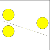
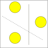
a. b. c. d.

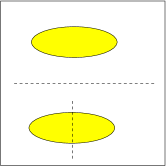
Figure 1: If data sets are not symmetric, idealized $K$-means is stable even if the number $K$ of clusters is too small (Figure a) or too large (Figure c). Instability of the wrong number of clusters only occurs in symmetric data sets (Figures b and d).

The starting point for the results in this section is the following observation (Ben-David et al., 2006). Consider the situation in Figure 1a. Here the data contains three clusters, but two of them are closer to each other than to the third cluster. Assume we run the idealized $K$-means algorithm with $K=2$ on such a data set. Separating the left two clusters from the right cluster (solid line) leads to a much better value of $Q^{(n)}_{K}$ than, say, separating the top two clusters from the bottom one (dashed line). Hence, as soon as we have a reasonable amount of data, idealized (!) $K$-means with $K=2$ always constructs the first solution (solid line). Consequently, it is stable in spite of the fact that $K=2$ is the wrong number of clusters. Note that this would not happen if the data set was symmetric, as depicted in Figure 1b. Here neither the solution depicted by the dashed line nor the one with the solid line is clearly superior, which leads to instability if the idealized $K$-means algorithm is applied to different samples. Similar examples can be constructed to detect that $K$ is too large, see Figure 1c and d. With $K=3$ it is clearly the best solution to split the big cluster in Figure 1c, thus clustering this data set is stable. In Figure 1d, however, due to symmetry reasons neither splitting the top nor the bottom cluster leads to a clear advantage. Again this leads to instability.

These informal observations suggest that unless the data set contains perfect symmetries, the idealized $K$-means algorithm is stable even if $K$ is wrong. This can be formalized with the following theorem.

Lemma 1 (Stability and global optima of the objective function)

Let $P$ be a probability distribution on $\mathbb{R}^{d}$ and $Q^{(\infty)}_{K}$ the limit $K$-means objective function as defined in Equation (2), for some fixed value $K>1$.

1. If $Q^{(\infty)}_{K}$ has a unique global minimum, then the idealized $K$-means algorithm is perfectly stable when $n\to\infty$, that is

   $$\lim_{n\to\infty}\operatorname{Instab}(K,n)=0.$$

2. If $Q^{(\infty)}_{K}$ has several global minima (for example, because the probability distribution is symmetric), then the idealized $K$-means algorithm is instable, that is

   $$\lim_{n\to\infty}\operatorname{Instab}(K,n)>0.$$

This theorem has been proved (in a slightly more general setting) in Ben-David et al. (2006) and Ben-David et al. (2007).

Proof sketch, Part 1. It is well known that if the objective function $Q^{(\infty)}_{K}$ has a unique global minimum, then the centers $c^{(n)}$ constructed by the idealized $K$-means algorithm on a sample of $n$ points almost surely converge to the true population centers $c^{(*)}$ as $n\to\infty$ (Pollard, 1981). This means that given some $\varepsilon>0$ we can find some large $n$ such that $c^{(n)}$ is $\varepsilon$-close to $c^{(*)}$ with high probability. As a consequence, if we compare two clusterings on different samples of size $n$, the centers of the two clusterings are at most $2\varepsilon$-close to each other. Finally, one can show that if the cluster centers of two clusterings are $\varepsilon$-close, then their minimal matching distance is small as well. Thus, the expected distance between the clusterings constructed on two samples of size $n$ becomes arbitrarily small and eventually converges to 0 as $n\to\infty$.
Part 2. For simplicity, consider the symmetric situation in Figure 1a. Here the probability distribution has three axes of symmetry. For $K=2$ the objective function $Q^{(\infty)}_{2}$ has three global minima $c^{(*1)},c^{(*2)},c^{(*3)}$ corresponding to the three symmetric solutions. In such a situation, the idealized $K$-means algorithm on a sample of $n$ points gets arbitrarily close to one of the global optima, that is $\min_{i=1,\ldots,3}d(c^{(n)},c^{(*i)})\to 0$ (Lember, 2003). In particular, the sequence $(c^{(n)})_{n}$ of empirical centers has three convergent subsequences, each of which converge to one of the global solutions. One can easily conclude that if we compare two clusterings on random samples, with probability 1/3 they belong to “the same subsequence” and thus their distance will become arbitrarily small. With probability 2/3 they “belong to different subsequences”, and thus their distance remains larger than a constant $a>0$. From the latter we can conclude that $\operatorname{Instab}(K,n)$ is always larger than $2a/3$. ☺

The interpretation of this theorem is distressing. The stability or instability of parameter $K$ does not depend on whether $K$ is “correct” or “wrong”, but only on whether the $K$-means objective function for this particular value $K$ has one or several global minima. However, the number of global minima is usually not related to the number of clusters, but rather to the fact that the underlying probability distribution has symmetries. In particular, if we consider “natural” data distributions, such distributions are rarely perfectly symmetric. Consequently, the corresponding functions $Q^{(\infty)}_{K}$ usually only have one global minimum, for any value of $K$. In practice this means that for a large sample size $n$, the idealized $K$-means algorithm is stable for any value of $K$. This seems to suggest that model selection based on clustering stability does not work. However, we will see later in Section 3 that this result is essentially an artifact of the idealized clustering setting and does not carry over to the realistic setting.

2 Refined convergence results for the case of a unique global minimum

Above we have seen that if, for a particular distribution $P$ and a particular value $K$, the objective function $Q^{(\infty)}_{K}$ has a unique global minimum, then the idealized $K$-means algorithm is stable in the sense that $\lim_{n\to\infty}\operatorname{Instab}(K,n)=0$. At first glance, this seems to suggest that stability cannot distinguish between different values $k_{1}$ and $k_{2}$ (at least for large $n$). However, this point of view is too simplistic. It can happen that even though both $\operatorname{Instab}(k_{1},n)$ and $\operatorname{Instab}(k_{2},n)$ converge to 0 as $n\to\infty$, this happens “faster” for $k_{1}$ than for $k_{2}$. If measured relative to the absolute values of $\operatorname{Instab}(k_{1},n)$ and $\operatorname{Instab}(k_{2},n)$, the difference between $\operatorname{Instab}(k_{1},n)$ and $\operatorname{Instab}(k_{2},n)$ can still be large enough to be “significant”.

The key in verifying this intuition is to study the limit process more closely. This line of work has been established by Shamir and Tishby in a series of papers (Shamir and Tishby, 2008a, b, 2009). The main idea is that instead of studying the convergence of $\operatorname{Instab}(k,n)$ one needs to consider the rescaled instability $\sqrt{n}\cdot\operatorname{Instab}(k,n)$. One can prove that the rescaled instability converges in distribution, and the limit distribution depends on $k$. In particular, the means of the limit distributions are different for different values of $k$. This can be formalized as follows.

Lemma 2 (Convergence of rescaled stability)

Assume that the probability distribution $P$ has a density $p$. Consider a fixed parameter $K$, and assume that the corresponding limit objective function $Q^{(\infty)}_{K}$ has a unique global minimum $c^{(*)}=(c^{(*)}_{1},\ldots,c^{(*)}_{K})$. The boundary between clusters $i$ and $j$ is denoted by $B_{ij}$. Let $m\in\mathbb{N}$, and $S_{n,1},\ldots,S_{n,2m}$ be samples of size $n$ drawn independently from $P$. Let $\mathcal{C}_{K}(S_{n,i})$ be the result of the idealized $K$-means clustering on sample $S_{n,i}$. Compute the instability as mean distance between clusterings of disjoint pairs of samples, that is

$$\overline{\operatorname{Instab}}(K,n):=\frac{1}{m}\sum_{i=1}^{m}d_{\text{MM}}\big{(}\mathcal{C}_{K}(S_{n,2i-1}),\mathcal{C}_{K}(S_{n,2i})\big{)}.$$ (3)

Then, as $n\to\infty$ and $m\to\infty$, the rescaled instability $\sqrt{n}\cdot\overline{\operatorname{Instab}}(K,n)$ converges in probability to

$$\text{RInstab}(K):=\sum_{1\leq i<j\leq K}\;\int_{B_{ij}}\;\frac{V_{ij}}{\|c^{(*)}_{i}-c^{(*)}_{j}\|}\;p(x)dx,$$ (4)

where $V_{ij}$ stands for a term describing the asymptotics of the random fluctuations of the cluster boundary between cluster $i$ and cluster $j$ (exact formula given in Shamir and Tishby, 2008a, 2009).

distribution of $d(\mathcal{C},\mathcal{C}^{\prime})$ distribution of $\sqrt{n}\cdot d(\mathcal{C},\mathcal{C}^{\prime})$ $k$ fixed $n=10^{2}$: $\xrightarrow{\text{scale with }\sqrt{n}=10}$ $n=10^{4}$: $\xrightarrow{\text{scale with }\sqrt{n}=100}$ $\downarrow$ $\downarrow$ $\downarrow$ $n=\infty$:

Figure 2: Different convergence processes. The left column shows the convergence studied in Theorem 1. As the sample size $n\to\infty$, the distribution of distances $d_{\text{MM}}(\mathcal{C},\mathcal{C}^{\prime})$ is degenerate, all mass is concentrated on 0. The right column shows the convergence studied in Theorem 2. The rescaled distances converge to a non-trivial distribution, and its mean (depicted by the cross) is positive. To go from the left to the right side one has to rescale by $\sqrt{n}$.

Note that even though the definition of instability in Equation (3) differs slightly from the definition in Equation (1), intuitively it measures the same quantity. The definition in Equation (3) just has the technical advantage that all pairs of samples are independent from one another.

Proof sketch. It is well known that if $Q^{(\infty)}_{K}$ has a unique global minimum, then the centers constructed by the idealized $K$-means algorithm on a finite sample satisfy a central limit theorem (Pollard, 1982). That is, if we rescale the distances between the sample-based centers and the true centers with the factor $\sqrt{n}$, these rescaled distances converges to a normal distribution as $n\to\infty$. When the cluster centers converge, the same can be said about the cluster boundaries. In this case, instability essentially counts how many points change side when the cluster boundaries move by some small amount. The points that potentially change side are the points close to the boundary of the true limit clustering. Counting these points is what the integrals $\int_{B_{ij}}...p(x)dx$ in the definition of RInstab take care of. The exact characterization of how the cluster boundaries “jitter” can be derived from the central limit theorem. This leads to the term $V_{ij}/\|c_{i}^{(*)}-c_{j}^{(*)}\|$ in the integral. $V_{ij}$ characterizes how the cluster centers themselves “jitter”. The normalization $\|c_{i}^{(*)}-c_{j}^{(*)}\|$ is needed to transform jittering of cluster centers to jittering of cluster boundaries: if two cluster centers are very far apart from each other, the cluster boundary only jitters by a small amount if the centers move by $\varepsilon$, say. However, if the centers are very close to each other (say, they have distance $3\varepsilon$), then moving the centers by $\varepsilon$ has a large impact on the cluster boundary. The details of this proof are very technical, we refer the interested reader to Shamir and Tishby 2008a, 2009. ☺

Let us briefly explain how the result in Theorem 2 is compatible with the result in Theorem 1. On a high level, the difference between both results resembles the difference between the law of large numbers and the central limit theorem in probability theory. The LLN studies the convergence of the mean of a sum of random variables to its expectation (note that $\operatorname{Instab}$ has the form of a sum of random variables). The CLT is concerned with the same expression, but rescaled with a factor $\sqrt{n}$. For the rescaled sum, the CLT then gives results on the convergence in distribution. Note that in the particular case of instability, the distribution of distances lives on the non-negative numbers only. This is why the rescaled instability in Theorem 2 is positive and not 0 as in the limit of $\operatorname{Instab}$ in Theorem 1. A toy figure explaining the different convergence processes can be seen in Figure 2.

Theorem 2 tells us that different parameters $k$ usually lead to different rescaled stabilities in the limit for $n\to\infty$. Thus we can hope that if the sample size $n$ is large enough we can distinguish between different values of $k$ based on the stability of the corresponding clusterings. An important question is now which values of $k$ lead to stable and which ones lead to instable results, for a given distribution $P$.

3 Characterizing stable clusterings

It is a straightforward consequence of Theorem 2 that if we consider different values $k_{1}$ and $k_{2}$ and the clustering objective functions $Q^{(\infty)}_{k_{1}}$ and $Q^{(\infty)}_{k_{2}}$ have unique global minima, then the rescaled stability values $\text{RInstab}(k_{1})$ and $\text{RInstab}(k_{2})$ can differ from each other. Now we want to investigate which values of $k$ lead to high stability and which ones lead to low stability.

Conclusion 3 (Instable clusterings)

Assume that $Q^{(\infty)}_{K}$ has a unique global optimum. If $\operatorname{Instab}(K,n)$ is large, the idealized $K$-means clustering tends to have cluster boundaries in high density regions of the space.

There exist two different derivations of this conclusion, which have been obtained independently from each other by completely different methods (Ben-David and von Luxburg, 2008, Shamir and Tishby, 2008b). On a high level, the reason why the conclusion tends to hold is that if cluster boundaries jitter in a region of high density, then more points “change side” than if the boundaries jitter in a region of low density.

First derivation, informal, based on Shamir and Tishby (2008b, 2009). Assume that $n$ is large enough such that we are already in the asymptotic regime (that is, the solution $c^{(n)}$ constructed on the finite sample is close to the true population solution $c^{(*)}$). Then the rescaled instability computed on the sample is close to the expression given in Equation (4). If the cluster boundaries $B_{ij}$ lie in a high density region of the space, then the integral in Equation (4) is large — compared to a situation where the cluster boundaries lie in low density regions of the space. From a high level point of view, this justifies the conclusion above. However, note that it is difficult to identify how exactly the quantities $p$, $B_{ij}$ and $V_{ij}$ influence RInstab, as they are not independent of each other.

Second derivation, more formal, based on Ben-David and von Luxburg (2008). A formal way to prove the conclusion is as follows. We introduce a new distance $d_{\text{boundary}}$ between two clusterings. This distance measures how far the cluster boundaries of two clusterings are apart from each other. One can prove that the $K$-means quality function $Q^{(\infty)}_{K}$ is continuous with respect to this distance function. This means that if two clusterings $\mathcal{C},\mathcal{C}^{\prime}$ are close with respect to $d_{\text{boundary}}$, then they have similar quality values. Moreover, if $Q^{(\infty)}_{K}$ has a unique global optimum, we can invert this argument and show that if a clustering $\mathcal{C}$ is close to the optimal limit clustering $\mathcal{C}^{*}$, then the distance $d_{\text{boundary}}(\mathcal{C},\mathcal{C}^{*})$ is small. Now consider the clustering $\mathcal{C}^{(n)}$ based on a sample of size $n$. One can prove the following key statement. If $\mathcal{C}^{(n)}$ converges uniformly (over the space of all probability distributions) in the sense that with probability at least $1-\delta$ we have $d_{\text{boundary}}(\mathcal{C}_{n},\mathcal{C})\leq\gamma$, then

$$\operatorname{Instab}(K,n)\leq 2\delta+P(T_{\gamma}(B)).$$ (5)

Here $P(T_{\gamma}(B))$ denotes the probability mass of a tube of width $\gamma$ around the cluster boundaries $B$ of $\mathcal{C}$. Results in Ben-David (2007) establish the uniform convergence of the idealized $K$-means algorithm. This proves the conjecture: Equation (5) shows that if $\operatorname{Instab}$ is high, then there is a lot of mass around the cluster boundaries, namely the cluster boundaries are in a region of high density.

For stable clusterings, the situation is not as simple. It is tempting to make the following conjecture.

Conjecture 4 (Stable clusterings)

Assume that $Q^{(\infty)}_{K}$ has a unique global optimum. If $\operatorname{Instab}(K,n)$ is “small”, the idealized $K$-means clustering tends to have cluster boundaries in low density regions of the space.

Argument in favor of the conjecture: As in the first approach above, considering the limit expression of RInstab reveals that if the cluster boundary lies in a low density area of the space, then the integral in RInstab tends to have a low value. In the extreme case where the cluster boundaries go through a region of zero density, the rescaled instability is even 0.

Argument against the conjecture: counter-examples! One can construct artificial examples where clusterings are stable although their decision boundary lies in a high density region of the space (Ben-David and von Luxburg, 2008). The way to construct such examples is to ensure that the variations of the cluster centers happen in parallel to cluster boundaries and not orthogonal to cluster boundaries. In this case, the sampling variation does not lead to jittering of the cluster boundary, hence the result is rather stable.

These counter-examples show that Conjecture 4 cannot be true in general. However, my personal opinion is that the counter-examples are rather artificial, and that similar situations will rarely be encountered in practice. I believe that the conjecture “tends to hold” in practice. It might be possible to formalize this intuition by proving that the statement of the conjecture holds on a subset of “nice” and “natural” probability distributions.

The important consequence of Conclusion 3 and Conjecture 4 (if true) is the following.

Conclusion 5

(Stability of idealized $K$-means detects whether $K$ is too large) Assume that the underlying distribution $P$ has $K$ well-separated clusters, and assume that these clusters can be represented by a center-based clustering model. Then the following statements tend to hold for the idealized $K$-means algorithm.

1. If $K$ is too large, then the clusterings obtained by the idealized $K$-means algorithm tend to be instable.

2. If $K$ is correct or too small, then the clusterings obtained by the idealized $K$-means algorithm tend to be stable (unless the objective function has several global minima, for example due to symmetries).

Given Conclusion 3 and Conjecture 4 it is easy to see why Conclusion 5 is true. If $K$ is larger than the correct number of clusters, one necessarily has to split a true cluster into several smaller clusters. The corresponding boundary goes through a region of high density (the cluster which is being split). According to Conclusion 3 this leads to instability. If $K$ is correct, then the idealized (!) $K$-means algorithm discovers the correct clustering and thus has decision boundaries between the true clusters, that is in low density regions of the space. If $K$ is too small, then the $K$-means algorithm has to group clusters together. In this situation, the cluster boundaries are still between true clusters, hence in a low density region of the space.

2 The actual $K$-means algorithm

Figure 3: Different initial configurations and the corresponding outcomes of the $K$-means algorithm. Figure a: the two boxes in the top row depict a data set with three clusters and four initial centers. Both boxes show different realizations of the same initial configuration. As can be seen in the bottom, both initializations lead to the same $K$-means clustering. Figure b: here the initial configuration is different from the one in Figure a, which leads to a different $K$-means clustering.

In this section we want to study the actual $K$-means algorithm. In particular, we want to investigate when and how it gets stuck in different local optima. The general insight is that even though, from an algorithmic point of view, it is an annoying property of the $K$-means algorithm that it can get stuck in different local optima, this property might actually help us for the purpose of model selection. We now want to focus on the effect of the random initialization of the $K$-means algorithm. For simplicity, we ignore sampling artifacts and assume that we always work with “infinitely many” data points; that is, we work on the underlying distribution directly.

The following observation is the key to our analysis. Assume we are given a data set with $K_{\text{true}}$ well-separated clusters, and assume that we initialize the $K$-means algorithm with $K_{\text{init}}\geq K_{\text{true}}$ initial centers. The key observation is that if there is at least one initial center in each of the underlying clusters, then the initial centers tend to stay in the clusters they had been placed in. This means that during the course of the $K$-means algorithm, cluster centers are only re-adjusted within the underlying clusters and do not move between them. If this property is true, then the final clustering result is essentially determined by the number of initial centers in each of the true clusters. In particular, if we call the number of initial centers per cluster the initial configuration, one can say that each initial configuration leads to a unique clustering, and different configurations lead to different clusterings; see Figure 3 for an illustration. Thus, if the initialization method used in $K$-means regularly leads to different initial configurations, then we observe instability.

In Bubeck et al. (2009), the first results in this direction were proved. They are still preliminary in the sense that so far, proofs only exist for a simple setting. However, we believe that the results also hold in a more general context.

Lemma 6 (Stability of the actual $K$-means algorithm)

Assume that the underlying distribution $P$ is a mixture of two well-separated Gaussians on $\mathbb{R}$. Denote the means of the Gaussians by $\mu_{1}$ and $\mu_{2}$.

1. Assume that we run the $K$-means algorithm with $K=2$ and that we use an initialization scheme that places one initial center in each of the true clusters (with high probability). Then the $K$-means algorithm is stable in the sense that with high probability, it terminates in a solution with one center close to $\mu_{1}$ and one center close to $\mu_{2}$.

2. Assume that we run the $K$-means algorithm with $K=3$ and that we use an initialization scheme that places at least one of the initial centers in each of the true clusters (with high probability). Then the $K$-means algorithm is instable in the sense that with probability close to 0.5 it terminates in a solution that considers the first Gaussian as cluster, but splits the second Gaussian into two clusters; and with probability close to 0.5 it does it the other way round.

Proof idea. The idea of this proof is best described with Figure 4. In the case of $K_{\text{init}}=2$ one has to prove that if the one center lies in a large region around $\mu_{1}$ and the second center in a similar region around $\mu_{2}$, then the next step of $K$-means does not move the centers out of their regions (in Figure 4, these regions are indicated by the black bars). If this is true, and if we know that there is one initial center in each of the regions, the same is true when the algorithm stops. Similarly, in the case of $K_{\text{init}}=3$, one proves that if there are two initial centers in the first region and one initial center in the second region, then all centers stay in their regions in one step of $K$-means. ☺

Figure 4: Stable regions used in the proof of Theorem 6. See text for details.

All that is left to do now is to find an initialization scheme that satisfies the conditions in Theorem 6. Luckily, we can adapt a scheme that has already been used in Dasgupta and Schulman (2007). For simplicity, assume that all clusters have similar weights (for the general case see Bubeck et al., 2009), and that we want to select $K$ initial centers for the $K$-means algorithm. Then the following initialization should be used:

Initialization (I):

• 1. Select $L$ preliminary centers uniformly at random from the given data set, where $L\approx K\log(K)$.

  2. Run one step of $K$-means, that is assign the data points to the preliminary centers and re-adjust the centers once.

  3. Remove all centers for which the mass of the assigned data points is smaller than $p_{0}\approx 1/L$.

  4. Among the remaining centers, select $K$ centers by the following procedure:

     1. Choose the first center uniformly at random.

     2. Repeat until $K$ centers are selected: Select the next center as the one that maximizes the minimum distance to the centers already selected.

One can prove that this initialization scheme satisfies the conditions needed in Theorem 6 (for exact details see Bubeck et al., 2009).

Lemma 7 (Initialization)

Assume we are given a mixture of $K_{\text{true}}$ well-separated Gaussians in $\mathbb{R}$, and denote the centers of the Gaussians by $\mu_{i}$. If we use the Initialization (I) to select $K_{\text{init}}$ centers, then there exist $K_{\text{true}}$ disjoint regions ${A}_{k}$ with $\mu_{k}\in{A}_{k}$, so that all $K_{\text{init}}$ centers are contained in one of the $A_{k}$ and

• if $K_{\text{init}}=K_{\text{true}}$, each $A_{k}$ contains exactly one center,

• if $K_{\text{init}}<K_{\text{true}}$, each $A_{k}$ contains at most one center,

• if $K_{\text{init}}>K_{\text{true}}$, each $A_{k}$ contains at least one center.

Proof sketch. The following statements can be proved to hold with high probability. By selecting $K_{\text{true}}\log(K_{\text{true}})$ preliminary centers, each of the Gaussians receives at least one of these centers. By running one step of $K$-means and removing the centers with too small mass, one removes all preliminary centers that sit on outliers. Moreover, one can prove that “ambiguous centers” (that is, centers that sit between two clusters) attract only few data points and will be removed as well. Next one shows that centers that are “unambiguous” are reasonably close to a true cluster center $\mu_{k}$. Consequently, the method for selecting the final center from the remaining preliminary ones “cycles though different Gaussians” before visiting a particular Gaussian for the second time. ☺

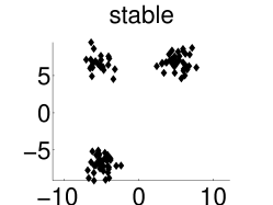
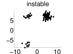
Figure 5: Illustration for the case where $K$ is too small. We consider two data sets that have been drawn from a mixture of three Gaussians with means $\mu_{1}=(-5,-7)$, $\mu_{2}=(-5,7)$, $\mu_{3}=(5,7)$ and unit variances. In the left figure, all clusters have the same weight $1/3$, whereas in the right figure the top right cluster has larger weight 0.6 than the other two clusters with weights 0.2 each. If we run $K$-means with $K=2$, we can verify experimentally that the algorithm is pretty stable if applied to points from the distribution in the left figure. It nearly always merges the top two clusters. On the distribution shown in the right figure, however, the algorithm is instable. Sometimes the top two clusters are merged, and sometimes the left two clusters.

When combined, the results of Theorems 6 and 7 show that if the data set contains $K_{\text{true}}$ well-separated clusters, then the $K$-means algorithm is stable if it is started with the true number of clusters, and instable if the number of clusters is too large. Unfortunately, in the case where $K$ is too small one cannot make any useful statement about stability because the aforementioned configuration argument does not hold any more. In particular, initial cluster centers do not stay inside their initial clusters, but move out of the clusters. Often, the final centers constructed by the $K$-means algorithm lie in between several true clusters, and it is very hard to predict the final positions of the centers from the initial ones. This can be seen with the example shown in Figure 5. We consider two data sets from a mixture of three Gaussians. The only difference between the two data sets is that in the left plot all mixture components have the same weight, while in the right plot the top right component has a larger weight than the other two components. One can verify experimentally that if initialized with $K_{\text{init}}=2$, the $K$-means algorithm is rather stable in the left figure (it always merges the top two clusters). But it is instable in the right figure (sometimes it merges the top clusters, sometimes the left two clusters). This example illustrates that if the number of clusters is too small, subtle differences in the distribution can decide on stability or instability of the actual $K$-means algorithm.

In general, we expect that the following statements hold (but they have not yet been proved in a context more general than in Theorems 6 and 7).

Conjecture 8 (Stability of the actual $K$-means algorithm)

Assume that the underlying distribution has $K_{\text{true}}$ well-separated clusters, and that these clusters can be represented by a center-based clustering model. Then, if one uses Initialization (I) to construct $K_{\text{init}}$ initial centers, the following statements hold:

• If $K_{\text{init}}=K_{\text{true}}$, we have one center per cluster, with high probability. The clustering results are stable.

• If $K_{\text{init}}>K_{\text{true}}$, different initial configurations occur. By the above argument, different configurations lead to different clusterings, so we observe instability.

• If $K_{\text{init}}<K_{\text{true}}$, then depending on subtle differences in the underlying distribution we can have either stability or instability.
  

3 Relationships between the results

In this section we discuss conceptual aspects of the results and relate them to each other.

1 Jittering versus jumping

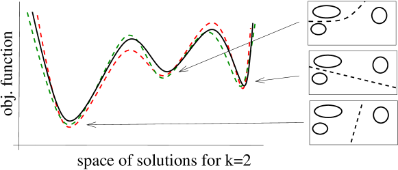
Figure 6: The $x$-axis depicts the space of all clusterings for a fixed distribution $P$ and for a fixed parameter $K$ (this is an abstract sketch only). The $y$-axis shows the value of the objective function of the different solutions. The solid line corresponds to the true limit objective function $Q^{(\infty)}_{K}$, the dotted lines show the sample-based function $Q^{(\infty)}_{K}$ on different samples. The idealized $K$-means algorithm only studies the jittering of the global optimum, that is how far the global optimum varies due to the sampling process. The jumping between different local optima is induced by different random initializations, as investigated for the actual $K$-means algorithm.

There are two main effects that lead to instability of the $K$-means algorithm. Both effects are visualized in Figure 6.

Jittering of the cluster boundaries. Consider a fixed local (or global) optimum of $Q^{(\infty)}_{K}$ and the corresponding clustering on different random samples. Due to the fact that different samples lead to slightly different positions of the cluster centers, the cluster boundaries “jitter”. That is, the cluster boundaries corresponding to different samples are slightly shifted with respect to one another. We call this behavior the “jittering” of a particular clustering solution. For the special case of the global optimum, this jittering has been investigated in Sections 2 and 3. It has been established that different parameters $K$ lead to different amounts of jittering (measured in terms of rescaled instability). The jittering is larger if the cluster boundaries are in a high density region and smaller if the cluster boundaries are in low density regions of the space. The main “source” of jittering is the sampling variation.

Jumping between different local optima. By “jumping” we refer to the fact that an algorithm terminates in different local optima. Investigating jumping has been the major goal in Section 2. The main source of jumping is the random initialization. If we initialize the $K$-means algorithm in different configurations, we end in different local optima. The key point in favor of clustering stability is that one can relate the number of local optima of $Q^{(\infty)}_{K}$ to whether the number $K$ of clusters is correct or too large (this has happened implicitly in Section 2).

2 Discussion of the main theorems

Theorem 1 works in the idealized setting. In Part 1 it shows that if the underlying distribution is not symmetric, the idealized clustering results are stable in the sense that different samples always lead to the same clustering. That is, no jumping between different solutions takes place. In hindsight, this result can be considered as an artifact of the idealized clustering scenario. The idealized $K$-means algorithm artificially excludes the possibility of ending in different local optima. Unless there exist several global optima, jumping between different solutions cannot happen. In particular, the conclusion that clustering results are stable for all values of $K$ does not carry over to the realistic $K$-means algorithm (as can be seen from the results in Section 2). Put plainly, even though the idealized $K$-means algorithm with $K=2$ is stable in the example of Figure 1a, the actual $K$-means algorithm is instable.
Part 2 of Theorem 1 states that if the objective function has several global optima, for example due to symmetry, then jumping takes place even for the idealized $K$-means algorithm and results in instability. In the setting of the theorem, the jumping is merely induced by having different random samples. However, a similar result can be shown to hold for the actual $K$-means algorithm, where it is induced due to random initialization. Namely, if the underlying distribution is perfectly symmetric, then “symmetric initializations” lead to the different local optima corresponding to the different symmetric solutions.

To summarize, Theorem 1 investigates whether jumping between different solutions takes place due to the random sampling process. The negative connotation of Part 1 is an artifact of the idealized setting that does not carry over to the actual $K$-means algorithm, whereas the positive connotation of Part 2 does carry over.

Theorem 2 studies how different samples affect the jittering of a unique solution of the idealized $K$-means algorithm. In general, one can expect that similar jittering takes place for the actual $K$-means algorithm as well. In this sense, we believe that the results of this theorem can be carried over to the actual $K$-means algorithm.
However, if we reconsider the intuition stated in the introduction and depicted in Figure 1, we realize that jittering was not really what we had been looking for. The main intuition in the beginning was that the algorithm might jump between different solutions, and that such jumping shows that the underlying parameter $K$ is wrong. In practice, stability is usually computed for the actual $K$-means algorithm with random initialization and on different samples. Here both effects (jittering and jumping) and both random processes (random samples and random initialization) play a role. We suspect that the effect of jumping to different local optima due to different initialization has higher impact on stability than the jittering of a particular solution due to sampling variation. Our reason to believe so is that the distance between two clusterings is usually higher if the two clusterings correspond to different local optima than if they correspond to the same solution with a slightly shifted boundary.

To summarize, Theorem 2 describes the jittering behavior of an individual solution of the idealized $K$-means algorithm. We believe that similar effects take place for the actual $K$-means algorithm. However, we also believe that the influence of jittering on stability plays a minor role compared to the one of jumping.

Theorem 6 investigates the jumping behavior of the actual $K$-means algorithm. As the source of jumping, it considers the random initialization only. It does not take into account variations due to random samples (this is hidden in the proof, which works on the underlying distribution rather than with finitely many sample points). However, we believe that the results of this theorem also hold for finite samples. Theorem 6 is not yet as general as we would like it to be. But we believe that studying the jumping behavior of the actual $K$-means algorithm is the key to understanding the stability of the $K$-means algorithm used in practice, and Theorem 6 points in the right direction.

Altogether, the results obtained in the idealized and realistic setting perfectly complement each other and describe two sides of the same coin. The idealized setting mainly studies what influence the different samples can have on the stability of one particular solution. The realistic setting focuses on how the random initialization makes the algorithm jump between different local optima. In both settings, stability “pushes” in the same direction: If the number of clusters is too large, results tend to be instable. If the number of clusters is correct, results tend to be stable. If the number of clusters is too small, both stability and instability can occur, depending on subtle properties of the underlying distribution.

Chapter 3 Beyond $K$-means

Most of the theoretical results in the literature on clustering stability have been proved with the $K$-means algorithm in mind. However, some of them hold for more general clustering algorithms. This is mainly the case for the idealized clustering setting.

Assume a general clustering objective function $Q$ and an ideal clustering algorithm that globally minimizes this objective function. If this clustering algorithm is consistent in the sense that the optimal clustering on the finite sample converges to the optimal clustering of the underlying space, then the results of Theorem 1 can be carried over to this general objective function (Ben-David et al., 2006). Namely, if the objective function has a unique global optimum, the clustering algorithm is stable, and it is instable if the algorithm has several global minima (for example due to symmetry). It is not too surprising that one can extend the stability results of the $K$-means algorithm to more general vector-quantization-type algorithms. However, the setup of this theorem is so general that it also holds for completely different algorithms such as spectral clustering. The consistency requirement sounds like a rather strong assumption. But note that clustering algorithms that are not consistent are completely unreliable and should not be used anyway.

Similarly as above, one can also generalize the characterization of instable clusterings stated in Conclusion 3, cf. Ben-David and von Luxburg (2008). Again we are dealing with algorithms that minimize an objective function. The consistency requirements are slightly stronger in that we need uniform consistency over the space (or a subspace) of probability distributions. Once such uniform consistency holds, the characterization that instable clusterings tend to have their boundary in high density regions of the space can be established.

While the two results mentioned above can be carried over to a huge bulk of clustering algorithms, it is not as simple for the refined convergence analysis of Theorem 2. Here we need to make one crucial additional assumption, namely the existence of a central limit type result. This is a rather strong assumption which is not satisfied for many clustering objective functions. However, a few results can be established (Shamir and Tishby, 2009): in addition to the traditional $K$-means objective function, a central limit theorem can be proved for other variants of $K$-means such as kernel $K$-means (a kernelized version of the traditional $K$-means algorithm) or Bregman divergence clustering (where one selects a set of centroids such that the average divergence between points and centroids is minimized). Moreover, central limit theorems are known for maximum likelihood estimators, which leads to stability results for certain types of model-based clusterings using maximum likelihood estimators. Still the results of Theorem 2 are limited to a small number of clustering objective functions, and one cannot expect to be able to extend them to a wide range of clustering algorithms.

Even stronger limitations hold for the results about the actual $K$-means algorithm. The methods used in Section 2 were particularly designed for the $K$-means algorithm. It might be possible to extend them to more general centroid-based algorithms, but it is not obvious how to advance further. In spite of this shortcoming, we believe that these results hold in a much more general context of randomized clustering algorithms. From a high level point of view, the actual $K$-means algorithm is a randomized algorithm due to its random initialization. The randomization is used to explore different local optima of the objective function. There were two key insights in our stability analysis of the actual $K$-means algorithm: First, we could describe the “regions of attraction” of different local minima, that is we could prove which initial centers lead to which solution in the end (this was the configurations idea). Second, we could relate the “size” of the regions of attraction to the number of clusters. Namely, if the number of clusters is correct, the global minimum will have a huge region of attraction in the sense that it is very likely that we will end in the global minimum. If the number of clusters is too large, we could show that there exist several local optima with large regions of attraction. This leads to a significant likelihood of ending in different local optima and observing instability.

We believe that similar arguments can be used to investigate stability of other kinds of randomized clustering algorithms. However, such an analysis always has to be adapted to the particular algorithm under consideration. In particular, it is not obvious whether the number of clusters can always be related to the number of large regions of attraction. Hence it is an open question whether results similar to the ones for the actual $K$-means algorithm also hold for completely different randomized clustering algorithms.

Chapter 4 Outlook

Based on the results presented above one can draw a cautiously optimistic picture about model selection based on clustering stability for the $K$-means algorithm. Stability can discriminate between different values of $K$, and the values of $K$ that lead to stable results have desirable properties. If the data set contains a few well-separated clusters that can be represented by a center-based clustering, then stability has the potential to discover the correct number of clusters.

An important point to stress is that stability-based model selection for the $K$-means algorithm can only lead to convincing results if the underlying distribution can be represented by center-based clusters. If the clusters are very elongated or have complicated shapes, the $K$-means algorithm cannot find a good representation of this data set, regardless what number $K$ one uses. In this case, stability-based model selection breaks down, too. It is a legitimate question what implications this has in practice. We usually do not know whether a given data set can be represented by center-based clusterings, and often the $K$-means algorithm is used anyway. In my opinion, however, the question of selecting the “correct” number of clusters is not so important in this case. The only way in which complicated structure can be represented using $K$-means is to break each true cluster in several small, spherical clusters and either live with the fact that the true clusters are split in pieces, or use some mechanism to join these pieces afterwards to form a bigger cluster of general shape. In such a scenario it is not so important what number of clusters we use in the $K$-means step: it does not really matter whether we split an underlying cluster into, say, 5 or 7 pieces.

There are a few technical questions that deserve further consideration. Obviously, the results in Section 2 are still somewhat preliminary and should be worked out in more generality. The results in Section 1 are large sample results. It is not clear what “large sample size” means in practice, and one can construct examples where the sample size has to be arbitrarily large to make valid statements (Ben-David and von Luxburg, 2008). However, such examples can either be countered by introducing assumptions on the underlying probability distribution, or one can state that the sample size has to be large enough to ensure that the cluster structure is well-represented in the data and that we don’t miss any clusters.

There is yet another limitation that is more severe, namely the number of clusters to which the results apply. The conclusions in Section 1 as well as the results in Section 2 only hold if the true number of clusters is relatively small (say, on the order of 10 rather than on the order of 100), and if the parameter $K$ used by $K$-means is in the same order of magnitude. Let us briefly explain why this is the case. In the idealized setting, the limit results in Theorems 1 and 2 of course hold regardless of what the true number of clusters is. But the subsequent interpretation regarding cluster boundaries in high and low density areas breaks down if the number of clusters is too large. The reason is that the influence of one tiny bit of cluster boundary between two clusters is negligible compared to the rest of the cluster boundary if there are many clusters, such that other factors might dominate the behavior of clustering stability. In the realistic setting of Section 2, we use an initialization scheme which, with high probability, places centers in different clusters before placing them into the same cluster. The procedure works well if the number of clusters is small. However, the larger the number of clusters, the higher the likelihood to fail with this scheme. Similarly problematic is the situation where the true number of clusters is small, but the $K$-means algorithm is run with a very large $K$. Finally, note that similar limitations hold for all model selection criteria. It is simply a very difficult (and pretty useless) question whether a data set contains 100 or 105 clusters, say.

While stability is relatively well-studied for the $K$-means algorithm, there does not exist much work on the stability of completely different clustering mechanisms. We have seen in Section 3 that some of the results for the idealized $K$-means algorithm also hold in a more general context. However, this is not the case for the results about the actual $K$-means algorithm. We consider the results about the actual $K$-means algorithm as the strongest evidence in favor of stability-based model selection for $K$-means. Whether this principle can be proved to work well for algorithms very different from $K$-means is an open question.

An important point we have not discussed in depth is how clustering stability should be implemented in practice. As we have outlined in Section 1 there exist many different protocols for computing stability scores. It would be very important to compare and evaluate all these approaches in practice, in particular as there are several unresolved issues (such as the normalization). Unfortunately, a thorough study that compares all different protocols in practice does not exist.

References

- Ben-David (2007) S. Ben-David. A framework for statistical clustering with constant time approximation algorithms for k-median and k-means clustering. Machine Learning, 66:243 – 257, 2007.
- Ben-David and von Luxburg (2008) S. Ben-David and U. von Luxburg. Relating clustering stability to properties of cluster boundaries. In R. Servedio and T. Zhang, editors, Proceedings of the 21rst Annual Conference on Learning Theory (COLT), pages 379 – 390. Springer, Berlin, 2008.
- Ben-David et al. (2006) S. Ben-David, U. von Luxburg, and D. Pál. A sober look on clustering stability. In G. Lugosi and H. Simon, editors, Proceedings of the 19th Annual Conference on Learning Theory (COLT), pages 5 – 19. Springer, Berlin, 2006.
- Ben-David et al. (2007) S. Ben-David, D. Pál, and H.-U. Simon. Stability of k -means clustering. In N. Bshouty and C. Gentile, editors, Conference on Learning Theory (COLT), pages 20–34. Springer, 2007.
- Ben-Hur et al. (2002) A. Ben-Hur, A. Elisseeff, and I. Guyon. A stability based method for discovering structure in clustered data. In Pacific Symposium on Biocomputing, pages 6 – 17, 2002.
- Bertoni and Valentini (2007) A. Bertoni and G. Valentini. Model order selection for bio-molecular data clustering. BMC Bioinformatics, 8(Suppl 2):S7, 2007.
- Bertoni and Valentini (2008) A. Bertoni and G. Valentini. Discovering multi-level structures in bio-molecular data through the Bernstein inequality. BMC Bioinformatics, 9(Suppl 2), 2008.
- Bittner et al. (2000) M. Bittner, P. Meltzer, Y. Chen, Y. Jiang, E. Seftor, M. Hendrix, M. Radmacher, R. Simon, Z. Yakhini, A. Ben-Dor, N. Sampas, E. Dougherty, E. Wang, F. Marincola, C. Gooden, J. Lueders, A. Glatfelter, P. Pollock, J. Carpten, E. Gillanders, D. Leja, K. Dietrich, C. Beaudry, M. Berens, D. Alberts, V. Sondak, M. Hayward, and J. Trent. Molecular classification of cutaneous malignant melanoma by gene expression profiling. Nature, 406:536 – 540, 2000.
- Bubeck et al. (2009) S. Bubeck, M. Meila, and U. von Luxburg. How the initialization affects the stability of the k-means algorithm. Draft, http://arxiv.org/abs/0907.5494, 2009.
- Dasgupta and Schulman (2007) S. Dasgupta and L. Schulman. A probabilistic analysis of EM for mixtures of separated, spherical gaussians. JMLR, 8:203–226, 2007.
- Efron and Tibshirani (1993) B. Efron and R. Tibshirani. An Introduction to the Bootstrap. Chapman & Hall, 1993.
- Fridlyand and Dudoit (2001) J. Fridlyand and S. Dudoit. Applications of resampling methods to estimate the number of clusters and to improve the accuracy of a clustering method. Technical Report 600, Department of Statistics, University of California, Berkeley, 2001.
- Hastie et al. (2001) T. Hastie, R. Tibshirani, and J. Friedman. The elements of statistical learning. Springer, New York, 2001.
- Kerr and Churchill (2001) M. K. Kerr and G. A. Churchill. Bootstrapping cluster analysis: Assessing the reliability of conclusions from microarray experiments. PNAS, 98(16):8961 – 8965, 2001.
- Lange et al. (2004) T. Lange, V. Roth, M. Braun, and J. Buhmann. Stability-based validation of clustering solutions. Neural Computation, 16(6):1299 – 1323, 2004.
- Lember (2003) J. Lember. On minimizing sequences for -centres. J. Approx. Theory, 120:20 – 35, 2003.
- Levine and Domany (2001) E. Levine and E. Domany. Resampling method for unsupervised estimation of cluster validity. Neural Computation, 13(11):2573 – 2593, 2001.
- Meila (2003) M. Meila. Comparing clusterings by the variation of information. In B. Schölkopf and M. Warmuth, editors, Proceedings of the 16th Annual Conference on Computational Learning Theory (COLT), pages 173–187. Springer, 2003.
- Möller and Radke (2006) U. Möller and D. Radke. A cluster validity approach based on nearest-neighbor resampling. In Proceedings of the 18th International Conference on Pattern Recognition (ICPR), pages 892–895, Washington, DC, USA, 2006. IEEE Computer Society.
- Pollard (1981) D. Pollard. Strong consistency of k-means clustering. Annals of Statistics, 9(1):135 – 140, 1981.
- Pollard (1982) D. Pollard. A central limit theorem for k-means clustering. Annals of Probability, 10(4):919 – 926, 1982.
- Shamir and Tishby (2008a) O. Shamir and N. Tishby. Model selection and stability in k-means clustering. In R. Servedio and T. Zhang, editors, Proceedings of the 21rst Annual Conference on Learning Theory (COLT), 2008a.
- Shamir and Tishby (2008b) O. Shamir and N. Tishby. Cluster stability for finite samples. In J.C. Platt, D. Koller, Y. Singer, and S. Rowseis, editors, Advances in Neural Information Processing Systems (NIPS) 21. MIT Press, Cambridge, MA, 2008b.
- Shamir and Tishby (2009) O. Shamir and N. Tishby. On the reliability of clustering stability in the large sample regime. In D. Koller, D. Schuurmans, Y. Bengio, and L. Bottou, editors, Advances in Neural Information Processing Systems 21 (NIPS). 2009.
- Smolkin and Ghosh (2003) M. Smolkin and D. Ghosh. Cluster stability scores for microarray data in cancer studies. BMC Bioinformatics, 36(4), 2003.
- Strehl and Ghosh (2002) A. Strehl and J. Ghosh. Cluster ensembles - a knowledge reuse framework for combining multiple partitions. JMLR, 3:583 – 617, 2002.
- Vinh and Epps (2009) N. Vinh and J. Epps. A novel approach for automatic number of clusters detection in microarray data based on consensus clustering. In Proceedings of the Ninth IEEE International Conference on Bioinformatics and Bioengineering, pages 84–91. IEEE Computer Society, 2009.