The Chemical Evolution
of the Monoceros Ring/Galactic Anticenter Stellar Structure

Abstract

The origin of the Galactic Anticenter Stellar Structure (GASS) or “Monoceros ring” — a low latitude overdensity at the edge of the Galactic disk spanning at least the second and third Galactic quadrants — remains controversial. Models for the origin of GASS fall generally into scenarios where it is either a part (e.g., warp) of the Galactic disk or it represents tidal debris from the disruption of a Milky Way (MW) satellite galaxy. To further constrain models for the origin of GASS, we derive chemical abundance patterns from high resolution spectra for 21 M giants spatially and kinematically identified with it. The abundances of the (mostly) $\alpha$ element titanium and s-process elements yttrium and lanthanum for these GASS stars are found to be lower at the same [Fe/H] than those for MW stars, but similar to those of stars in the Sagittarius stream, other dwarf spheroidal galaxies, and the Large Magellanic Cloud. This demonstrates that GASS stars have a chemical enrichment history typical of dwarf galaxies — and unlike those of typical MW stars (at least MW stars near the Sun). Nevertheless, these abundance results cannot definitively rule out the possibility that GASS was dynamically created out of a previously formed, outer MW disk because $\Lambda$CDM-based structure formation models show that galactic disks grow outward by accretion of dwarf galaxies. On the other hand, the chemical patterns seen in GASS stars do provide striking verification that accretion of dwarf galaxies has indeed happened at the edge of the MW disk.

1 Introduction

The Galactic Anticenter Stellar Structure (GASS), also called the “Monoceros Stream” or “Monoceros Ring”, was discovered as several overdensities of presumed main sequence turnoff stars with F-type colors in the Sloan Digital Sky Survey (SDSS; Newberg et al. 2002) at a mean distance of $\sim$$11$ kpc from the Sun in the general region of the Galactic anticenter direction in Monoceros. Subsequent study of this arc-like structure with 2MASS M giant tracing (Majewski et al. 2003, hereafter M03; Rocha-Pinto et al. 2003, hereafter RP03) and spectroscopy (Crane et al. 2003, hereafter C03), with the Isaac Newton Telescope Wide Field Camera (INT/WFC) (e.g., Ibata at al. 2003, hereafter I03), and with SDSS photometry and spectroscopy (e.g., Yanny et al. 2003, hereafter Y03) has shown the low latitude GASS ring spans at least the second and third Galactic quadrants and a wide metallicity range, from [Fe/H]= $-1.6\pm 0.3$ (Y03) to $-0.4\pm 0.3$ (C03).

The origin of GASS remains controversial. Models for its formation fall into one of two general categories: (1) scenarios where GASS is a part of the Milky Way (MW) disk seen at higher latitudes due to the disk warp or some other dynamical excitation of the disk (Ibata at al. 2003; Momany et al.2006; Kazantzidis et al. 2008; Younger et al. 2008), versus (2) those scenarios where GASS represents a tidal debris stream from the disruption of a MW satellite galaxy (Ibata at al. 2003; Y03; C03; RP03; Helmi et al. 2003; Frinchaboy et al. 2004; Martin et al. 2004a; Conn et al. 2007; Peñarrubia et al. 2005; Rocha-Pinto et al. 2006). Furthermore, Martin et al. (2004a, 2004b) claim to find an overdensity in Canis Major (CMa, $l\sim 240^{\circ}$) and assume it is the progenitor of GASS, although the existence of this overdensity itself has been challenged (e.g., Momany et al. 2006; Rocha-Pinto et al. 2006; Mateu et al. 2009). While several candidates for a parent system to the putative tidal stream have been proffered (Martin et al. 2004a, 2004b; Rocha-Pinto et al. 2006), the basic issue of a disk versus stream origin is still hotly debated (Martin et al. 2004b; Momany et al. 2006; Conn et al. 2007). It is interesting to note that Bonifacio et al. (2000) suggested that a small galaxy might be hidden in this region of the Galaxy based on their derived distance to Nova V 1493 Aql.

In this Letter we gain insights into the origin of the GASS system by exploring its chemistry. Because chemical enrichment histories are a function of environment as well as other, stochastic processes, it is expected that stars that formed originally in different, isolated environments will bear significantly different chemical imprints in their spectra. Such differences have already been demonstrated by, for example, depressed $\alpha$-element and s-process abundances in dwarf galaxies compared to nearby MW stars (e.g., Shetrone et al. 2003; Venn et al. 2004; Geisler et al. 2005; Chou et al. 2010, hereafter C10). Here we analyze the abundances of the primarily $\alpha$-element titanium (Ti) and s-process elements yttrium (Y) and lanthanum (La) in GASS M giant candidates, and we compare those abundances with those of the Sagittarius (Sgr) dwarf galaxy, the Large Magellanic Cloud (LMC) and other dwarf spheroidal (dSph) satellite galaxies of the MW (including Sculptor, Carina, Draco, Ursa Minor, Fornax, Sextans and Leo I). A comparison to the Sgr and LMC systems is particularly apropos in the study of GASS because Sgr and the LMC exhibit some similar properties to GASS, including relatively high metallicities and the presence of M giants (C03; M03; RP03; C10). It is interesting to know whether these similarities between the GASS, Sgr and LMC systems extend to their detailed chemical patterns, or if GASS chemistry more closely resembles that of the typically more metal-rich MW disk.

2 Observations and Analysis

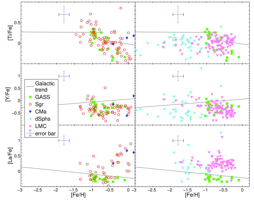
Figure 1: The distribution as a function of [Fe/H] of the abundance ratios (top panel) [Ti/Fe], (middle) [Y/Fe] and (bottom) [La/Fe] for GASS stars (green squares), comparing with Sgr (red open circles) and CMa stars (blue diamonds) in the left panels, and dSph (cyan triangles) and LMC stars (pink triangles) in the right panels. The Sgr data come from C10, the CMa data are from Sbordone et al. (2005), the dSph data are from Shetrone et al. (2001; 2003), Sadakane et al. (2004) and Geisler et al. (2005), the LMC stars are from Johnson et al. (2006), Pompéia et al. (2008) and Mucciarelli et al. (2008), and the lines represent the linear fits to the MW star distribution (see discussion in C10). The MW data have been taken from Gratton & Sneden (1994), Fulbright (2000), Johnson (2002) and Reddy et al. (2003). The typical error bars are shown to the left of each panel in blue.

We obtained high resolution spectra of 21 stars spatially coincident (i.e. by position on the sky and projected distance) with the GASS system based on M03’s work, but, additionally, vetted for proper GASS radial velocity by C03. The data were taken with the Echelle spectrograph mounted on the Kitt Peak National Observatory Mayall 4-m telescope and the SARG spectrograph on the Telescopio Nazionale Galileo (TNG) 3.5-m telescope, having resolutions of $R=35,000$ and 46,000, respectively. Examples of spectra from each instrument can be seen in Figure 3 of Chou et al. (2007, hereafter C07) and Figure 1 of C10.

Analysis of the spectra follows very closely that used in the analysis of Sgr system M giants described in C07 and C10. We focus on measuring equivalent widths (EWs) of eleven Fe I lines, two Ti I lines, and one Y II line, and analyzing by way of spectral synthesis one La II line; these lines all lie in a particular part of the spectrum (7440-7590 Å ) previously investigated by, e.g., Smith & Lambert (1985) in their spectroscopic exploration of M giants.

Our derivation of the abundances of these elements uses the LTE code MOOG (Sneden 1973) and follows the same procedures described in C07 and C10, where the excitation potentials and $gf$-values adopted for each line are also given. These particular chemical elements were chosen not only because they have well-defined, measurable spectral lines in M giants, but also because they show distinctive abundance ratios (relative to Fe) between different dwarf galaxies and, as a group, when these dwarf systems are compared to the MW.

The model atmospheres adopted here are the same as in C07 and C10, and were generated by linear interpolation from the grids of ATLAS9 models (Castelli & Kurucz 2003). We used the ODFNEW models with a microturbulence of 2 km s^-1 and no convective overshooting in our analysis.

Table 1 summarizes the targets, their equatorial and Galactic coordinate positions, the velocity in the Galactic Standard of Rest frame ($v_{GSR}$), the spectrograph with which each target was observed and on what date, and the $S/N$ of each spectrum. The $v_{GSR}$ values were derived by cross-correlating the echelle order that we used for the chemical analyses against the same order for several radial velocity standard stars taken from the Astronomical Almanac. The estimated standard deviations of the velocities are $\sim 1.2$ km s^-1 for the KPNO spectra, and 0.5 km s^-1 for the SARG spectra. The $S/N$ was determined using the total photoelectron count level at 7490Å. Table 2 lists the apparent magnitudes $K_{s}$, dereddened $(J-K_{s})_{o}$ colors, and the derived abundance results for these GASS stars. The columns in Table 2 give the derived effective temperature using the Houdashelt et al. (2000) color-temperature relation applied to the 2MASS $(J-K_{s})_{o}$ color, and the derived values of the surface gravity ($\log{g}$), microturbulence ($\xi$), abundance $A$(X), and abundance ratios [Fe/H] or [X/H] for each element X as well as the standard deviation in the abundance determinations. The microturbulence is determined by minimizing the dependence between the derived Fe abundance and the Fe I EW for the different lines. The standard deviation represents the line-to-line scatter of the EW measures (for Fe, Ti and Y), or different continuum level adjustments (for La), as discussed in C07 and C10. The final measured EWs of the lines we analyzed for each of the GASS spectra will be given elsewhere (M.-Y. Chou et al., in prep.).

Abundance uncertainties were estimated for three sample GASS stars by varying the model atmosphere in effective temperature ($T_{\rm eff}$), surface gravity (log $g$) and microturbulent velocity ($\xi$). The sensitivity of abundances to these stellar parameters is given in Table 3. The uncertainty in effective temperature is $\sim$$\pm 80$ K based on the Houdashelt et al. (2000a,b) color-temperature relation. The uncertainty in the surface gravity is $\sim$$\pm 0.15$ dex, which also comes from the uncertainty in the effective temperature, propagated along the corresponding isochrone (see C07). The uncertainty in microturbulent velocity is $\sim$$\pm 0.1$ km s^-1, which we estimate from the relation of abundance $A$(Fe) versus Fe I EW for different lines. The final, estimated errors propagated from these uncertainties in the stellar parameters are 0.08, 0.11, 0.07, 0.05 for [Fe/H], [Ti/Fe], [Y/Fe], and [La/Fe], respectively. Finally, the EW measurement uncertainty is $\sim 3$-$5$ mÅ , estimated by the equation given in Smith et al. (2000). Combining the uncertainties in stellar parameters and EW measurements, we estimate the net abundance errors to be no more than $\sim 0.2$ dex for each element ratio in Table 2.

3 Results and Discussion

Figure 1 compares the derived distributions of [Ti/Fe], [Y/Fe], and [La/Fe] as a function of [Fe/H] for the GASS, Sgr stars (the latter from C07 and C10), those of the LMC and other dSph galaxies. The lines represent linear fits to the abundance distributions of nearby disk and halo stars (see C10). As may be seen in the left panels, in all cases (1) the nearby MW and GASS abundance patterns are not coincident, while (2) the distribution of abundances and metallicities for GASS and Sgr stars is very similar, except for the [La/Fe] patterns at the highest metallicities (where the relative patterns suggest that Sgr stars probably enriched somewhat more slowly than GASS stars). The overall similarity of GASS and Sgr patterns shows that the stars in these two systems had a rather similar enrichment history, and may provide at least circumstantial evidence that the GASS/Mon stars originally derived from an accreted dwarf galaxy similar to that represented by the Sgr dwarf galaxy.

On the other hand, Sbordone et al. (2005) showed the chemical abundances for three giant star candidates of the CMa overdensity. The higher [Ti/Fe] and [La/Fe] of these CMa stars compared to those from GASS in the left panels of Figure 1 may suggest the CMa overdensity is not part of the GASS. The chemistry of these CMa stars more closely resembles that for the Sgr dSph, but, interestingly, also differs from that of Galactic disk stars (see the comparison with the Galactic trends). Though more data on CMa stars are certainly warranted, the results shown here support the conclusion that CMa and GASS are distinct from one another (e.g., Mateu et al. 2009).

However, we note that these CMa stars for which Sbordone et al. (2005) have measured abundances are K giants.. Some of the systematic differences between the Ti abundances derived for K and M giants in the different studies could partially come from the fact that these abundances were computed in LTE. In addition to possible differences due to NLTE effects in Ti I transitions between K and M giants, it is worth noting that the Ti I lines used by Sbordone et al. (2005) and this study are all different, making detailed comparisons subject to some uncertainty due to using different spectral lines, which may have different NLTE corrections.

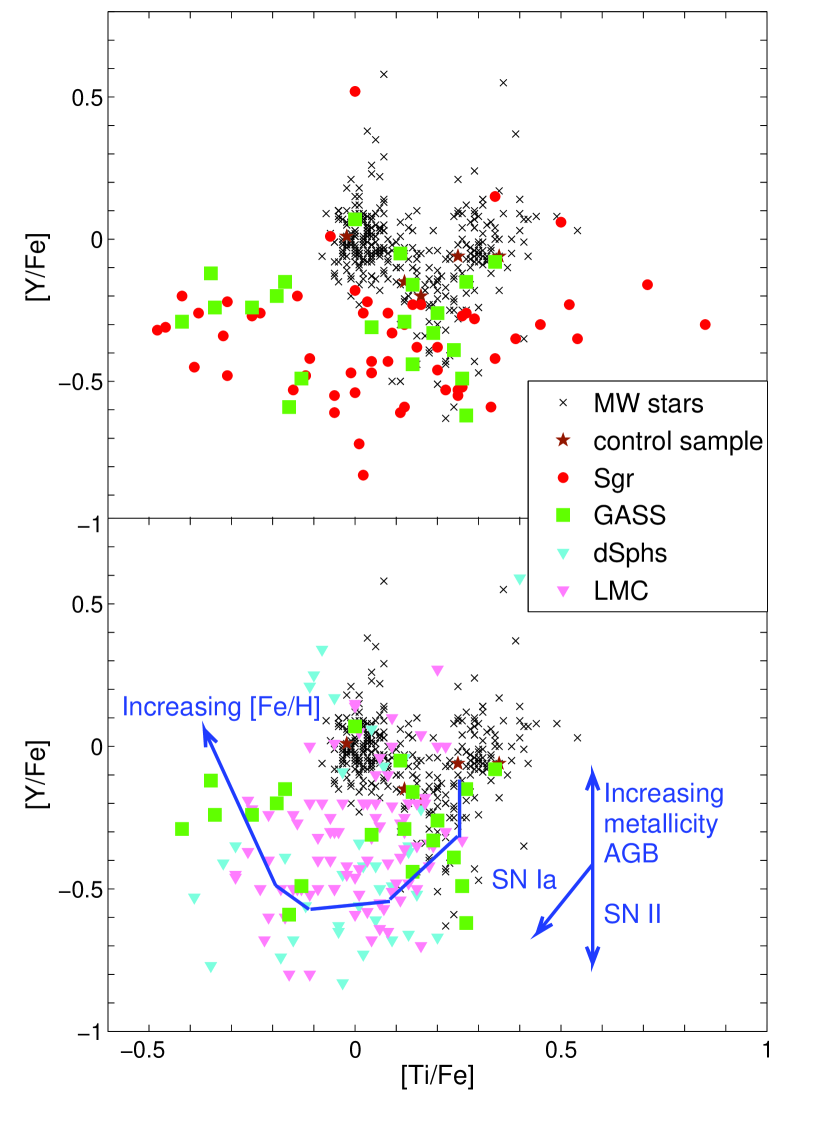
Figure 2: (Top panel) Distribution of [Y/Fe] versus [Ti/Fe] for the GASS stars, compared with the Milky Way (black crosses) and Sgr (red filled circles). The brown star symbols show the “control sample” stars for our survey (C10). The MW data are from Fulbright (2000), Johnson (2002) and Reddy et al. (2003). The Sgr data are from Sbordone et al. (2007) and C10. The MW stars lie within the well-defined horseshoe-shaped distribution near the top. (Bottom panel) Distribution of [Y/Fe] versus [Ti/Fe] for the GASS stars, compared with the Milky Way (black crosses), other dSph (cyan triangles) and LMC stars (pink triangles). The arrows illustrate schematically which way various stellar contributions would move the element ratios.

In the right panels of Figure 1 it is obvious that GASS goes to higher [Fe/H] than the LMC and especially the other dSphs, but most stars in all of these systems have similarly low [Ti/Fe] and [Y/Fe] compared to the MW. This resemblance is reinforced by Figure 2, which shows the distribution of [Y/Fe] versus [Ti/Fe] for GASS, Sgr, other dSph, LMC and MW stars. As may be seen, the distribution of most of the GASS stars in this observational plane resembles those for Sgr, other dSphs and the LMC, which indicates they share the same chemical patterns and may have similar chemical evolution histories. Figure 2 also further demonstrates the differences in chemical evolution between the GASS stars and the nominal MW populations.

On the other hand, the [La/Fe] ratios for most dSph stars, as well as more metal-rich LMC and Sgr stars, are enhanced compared to the MW, in strong contrast to what is observed among our (metal-rich) GASS stars. In this way GASS distinguishes itself from all other MW satellites with known [La/Fe] measures.

As discussed in C10, the distinctive enrichment history of a stellar system leads to particular abundance patterns in its stars, and therefore “chemical fingerprinting” can help identify tidally stripped and captured stars in the Galactic field. For instance, $\alpha$-elements are mainly produced from Type II supernovae (SN II) while iron is synthesized largely by Type Ia supernovae (SN Ia). So [$\alpha$/Fe] is high in the early enrichment process of a stellar system until SN Ia ignite after the first $\sim$$1$ Gyr. Ti acts primarily as an $\alpha$ element (although it also can be produced in SN Ia). The chemical patterns of the $\alpha$-elements (e.g., Ti) and s-process elements (e.g., Y and La) may demonstrate differences in the (early) star formation rate (SFR) between the progenitor GASS, Sgr, other dSph, LMC and MW systems.

The straight arrows on Figure 2 illustrate schematically which way these various supernovae yields move the combinations of element ratios in that abundance plane. As the straight arrows in Figure 2 show, SN II produce little Y but some Fe, so that [Y/Fe] decreases in the early enrichment stage, while Ti is made in proportion to Fe (at a super-solar level). After SN Ia occur, Fe is produced more prodigiously compared to Ti and other $\alpha$ elements, and stars initially move to the left and slightly down in Figure 2. Following the subsequent contribution of low mass AGB yields, the [Y/Fe] starts to increase with increasing [Fe/H] (see curved [Fe/H] arrow). The lower [$\alpha$/Fe] trend for GASS compared to the MW at the same [Fe/H] indicates a slower initial GASS SFR, which allows much of the iron from SN Ia to be introduced at lower overall metallicities. This is a feature that can be seen in many dSph galaxies as well as the LMC (Figs. 1 and 2; also see, e.g., Shetrone et al. 2003; Venn et al. 2004; Geisler et al. 2005; Pompéia et al. 2008; C10).

Meanwhile the s-process elements are primarily generated in low mass asymptotic giant branch (AGB) stars. The delay in the introduction of significant s-process element yields leads to the eventual upturn in the evolutionary track (followed by the mean [Fe/H] level) seen in Figure 2. These AGB stars produce heavier s-process elements like La more efficiently than lighter species such as Y in more metal-poor environments (see the review by Busso, Gallino, & Wasserburg 1999). C10 has shown underabundant trends in [Y/Fe] for most Sgr stars compared to the MW, and an upturn in [La/Fe] for Sgr at [Fe/H]$>$$-0.5$ (Fig. 1). The latter trend suggests a slow enrichment history so that the yields from low-metallicity AGB stars have enough time to contaminate the interstellar medium and leave their signature on the metal-rich Sgr populations (Venn et al. 2004; Pompéia et al. 2008). The left middle panel in Figure 1 shows the similarly lower trends of [Y/Fe] for Sgr and GASS compared with the MW, which may suggest the GASS and Sgr progenitors are from similar metal-poor environments. However, the left bottom panel of Figure 1 shows no apparent upturn in [La/Fe] for GASS stars as seen in Sgr. This indicates that GASS may have enriched somewhat faster than Sgr, which could explain why we do not see the low-metallicity AGB yields in the present GASS stellar population.

In the end, that the chemical characteristics of $\alpha$ and s-process elements for our GASS stars are very similar to those seen in Sgr and other satellite galaxies (see Figs. 1-2) suggests a dSph-like environment for the origin of GASS stars, with the closest matches to the LMC and Sgr as prototypes when overall metallicity is also considered. In addition, Lanfranchi, Matteucci & Cescutti (2008) predict subsolar [Y/Fe] and [La/Fe] for dSphs in their standard model, which further reinforces that GASS stars enriched in a dSph-like environment.

However, we hasten to add that this chemical connection of GASS stars to a dwarf galaxy origin alone cannot resolve the debate over whether GASS/Mon is presently a distinct tidal stream or a warp or other structure generated from a previously formed, outer MW disk because it is now believed that galactic disks grow outward by the accretion of dwarf galaxies. For example, the chemical abundance studies of MW disk red giants and Cepheids by Yong et al. (2005, 2006) and Carney et al. (2005) suggest that the outer Galactic disk may have formed via merger events. Numerical simulations of galaxy evolution in a Cold Dark Matter context also support that galactic disks grow outward by the accretion of dwarf galaxies (Abadi et al. 2003; Brook et al. 2007; Read et al. 2008). Finally, recent studies propose that flyby satellite encounters could cause ringlike features in the outer disk (Kazantzidis et al. 2008; Younger et al. 2008). Thus, it may well be that the outer disk could be made from recently acquired debris of multiple Sgr-like systems that then through dynamical processes transformed into what we see as the GASS/Mon structure today. A more interesting chemical discriminant between the competing GASS/Mon formation scenarios outlined in §1 would be to test GASS chemistry against that of bona fide outer disk stars (see M.-Y. Chou et al., in prep.) to see if GASS is pre- or post-outer MW disk material.

Table 1: The Program Stars

Star No.	$\alpha$(2000)	$\delta$(2000)	$l$	$b$	$v_{\rm gsr}$	Spectrograph	Observation	S/N
	(deg)	(deg)	(deg)	(deg)	(km s-1)		UT Date
GASS
$J02340206+8446368$	38.50857	84.77688	125.37	22.40	56.7	ECHLR	2006 Dec 06	82
$J05144786+8605371$	78.69943	86.09364	126.88	25.47	66.7	ECHLR	2006 Dec 05	87
$J06044611+3942523$	91.19213	39.71452	172.60	8.80	-13.1	SARG	2004 Mar 11	40
$J06341077+2421564$	98.54485	24.36566	189.25	7.30	-26.0	SARG	2004 Mar 10	39
$J06402752+5944247$	100.11467	59.74018	155.78	21.86	20.5	ECHLR	2006 Dec 08	93
$J06463306+5521444$	101.63773	55.36232	160.54	21.37	57.5	ECHLR	2006 Dec 07	104
$J07003934+4730561$	105.16393	47.51558	169.27	21.13	27.3	ECHLR	2004 May 09	47
$J07022522+2823272$	105.60508	28.39090	188.24	14.73	-29.7	ECHLR	2004 May 07	60
$J07041061+3911224$	106.04421	39.18957	177.89	19.05	-16.6	ECHLR	2004 May 06	66
$J07052136+6012353$	106.33901	60.20981	156.10	25.00	7.7	ECHLR	2006 Dec 08	100
$J07074384+1319528$	106.93267	13.33134	202.79	9.59	-30.7	SARG	2004 Mar 12	38
$J07110708+5027276$	107.77949	50.45766	166.73	23.59	36.8	ECHLR	2006 Dec 06	112
$J07165539+5409046$	109.23078	54.15129	163.01	25.31	15.3	ECHLR	2006 Dec 08	95
$J07314622+5936181$	112.94259	59.60503	157.34	28.17	28.9	ECHLR	2004 May 08	63
$J07393712+3315325$	114.90466	33.25903	186.39	23.91	-38.7	ECHLR	2004 May 08	66
$J08205065+1523392$	125.21104	15.39422	208.50	26.57	-44.7	ECHLR	2004 May 06	82
$J08501690+2545291$	132.57042	25.75807	199.75	36.54	-12.1	ECHLR	2004 May 07	60
$J08534628+0604280$	133.44281	6.07444	221.99	29.90	-53.8	ECHLR	2004 May 05	61
$J09122898+2632290$	138.12073	26.54140	200.41	41.56	-21.6	ECHLR	2004 May 05	63
$J09164929+5630048$	139.20537	56.50134	159.79	42.17	12.0	ECHLR	2004 May 05	64
$J22260469+8218595$	336.51956	82.31651	118.07	20.86	58.3	ECHLR	2006 Dec 06	84

Table 2: Stellar Parameters and Chemical Abundances for the Program Stars

Star No.	$\!K_{s,o}\,$	$\,(J-K_{s})_{o}\!$	$T_{\rm eff}$	logg		$\xi$	A(Fe)	[Fe/H]	A(Ti)	[Ti/Fe]		A(Y)	[Y/Fe]		A(La)		[La/Fe]
			(K)	(${\rm cm\,s^{-2}}$)		(${\rm km\,s^{-1}}$)
Sun	$\cdots$	$\cdots$	$\cdots$	$\cdots$		$\cdots$	7.45	$\cdots$	4.90	$\cdots$		2.21	$\cdots$		1.13		$\cdots$
GASS
$J02340206+8446368$	9.83	1.07	3750	0.4		1.37	6.87	$-0.58/0.12$	4.44	$0.12/0.06$		1.34	$-0.29/0.07$		0.32		$-0.34/0.02$
$J05144786+8605371$	9.57	1.05	3750	0.3		1.43	6.73	$-0.72/0.10$	4.01	$-0.17/0.07$		1.34	$-0.15/0.01$		0.23		$-0.28/0.04$
$J06044611+3942523$	9.79	1.01	3850	0.6		2.05	6.89	$-0.56/0.08$	4.21	$-0.13/$ $\cdots$		1.16	$-0.49/$ $\cdots$		$\cdots$		$\cdots$ $/$ $\cdots$
$J06341077+2421564$	9.41	1.05	3750	0.3		2.05	6.78	$-0.67/0.09$	4.27	$0.04/0.05$		1.23	$-0.31/$ $\cdots$		0.30		$-0.26/0.03$
$J06402752+5944247$	9.12	1.12	3650	0.4		1.66	7.02	$-0.43/0.09$	4.12	$-0.35/0.07$		1.66	$-0.12/0.10$		0.47		$-0.34/0.01$
$J06463306+5521444$	10.01	1.06	3750	0.9		1.49	7.35	$-0.10/0.13$	4.46	$-0.34/0.00$		1.87	$-0.24/0.07$		0.84		$-0.29/0.09$
$J07003934+4730561$	8.99	1.20	3700	0.0	(-)	1.98	6.50	$-0.95/0.10$	4.06	$0.11/0.07$		1.21	$-0.05/0.02$		0.11		$-0.17/0.02$
$J07022522+2823272$	8.63	1.21	3550	0.0	(-)	1.92	6.41	$-1.04/0.08$	4.13	$0.27/0.14$		0.55	$-0.62/0.16$		$-0.08$		$-0.27/0.04$
$J07041061+3911224$	7.86	1.21	3550	0.0	(-)	1.88	6.46	$-0.99/0.09$	4.25	$0.34/0.17$		1.14	$-0.08/0.13$		$-0.28$		$-0.52/0.04$
$J07052136+6012353$	9.79	1.02	3800	0.8		1.74	7.15	$-0.30/0.11$	4.41	$-0.19/0.01$		1.71	$-0.20/0.04$		0.74		$-0.19/0.01$
$J07074384+1319528$	9.13	1.09	3700	0.2		2.00	6.84	$-0.61/0.06$	4.43	$0.14/0.18$		1.16	$-0.44/$ $\cdots$		0.43		$-0.19/0.08$
$J07110708+5027276$	9.62	1.03	3800	0.8		1.66	7.15	$-0.30/0.12$	4.35	$-0.25/0.01$		1.67	$-0.24/0.05$		0.71		$-0.22/0.04$
$J07165539+5409046$	10.08	1.01	3850	0.3		1.95	6.55	$-0.90/0.11$	4.14	$0.14/0.08$		1.15	$-0.16/$ $\cdots$		0.17		$-0.16/0.02$
$J07314622+5936181$	9.12	1.09	3700	0.0	(-)	1.96	6.44	$-1.01/0.08$	3.89	$0.00/0.03$		1.31	$0.07/0.12$		0.12		$-0.10/0.01$
$J07393712+3315325$	8.85	1.14	3650	0.0	(-)	1.80	6.52	$-0.93/0.09$	4.17	$0.20/0.09$		1.02	$-0.26/0.31$		0.10		$-0.20/0.04$
$J08205065+1523392$	8.05	1.12	3700	0.0	(-)	1.60	6.51	$-0.94/0.06$	4.23	$0.27/0.06$		1.12	$-0.15/0.04$		0.03		$-0.26/0.05$
$J08501690+2545291$	9.27	1.15	3650	0.0	(-)	1.70	6.65	$-0.80/0.07$	3.94	$-0.16/0.08$		0.82	$-0.59/0.09$		0.18		$-0.25/0.03$
$J08534628+0604280$	9.30	1.11	3700	0.0	(-)	1.64	6.53	$-0.92/0.07$	4.22	$0.24/0.00$		0.90	$-0.39/$ $\cdots$		$-0.02$		$-0.33/0.03$
$J09122898+2632290$	9.28	1.08	3700	0.0		1.32	6.69	$-0.76/0.07$	4.40	$0.26/0.03$		0.96	$-0.49/0.10$		$-0.14$		$-0.61/0.04$
$J09164929+5630048$	8.98	1.11	3700	0.0	(-)	1.80	6.48	$-0.97/0.09$	4.12	$0.19/0.05$		0.91	$-0.33/$ $\cdots$		0.04		$-0.22/0.11$
$J22260469+8218595$	9.39	1.13	3650	0.5		1.49	7.00	$-0.45/0.10$	4.03	$-0.42/0.01$		1.47	$-0.29/$ $\cdots$		$\cdots$		$\cdots$ $/$ $\cdots$

Table 3: Sensitivity of Abundances to Stellar Parameters

Star Name	$\Delta T_{\rm eff}=+100$	$\Delta$log g$=+0.2$	$\Delta\xi=+0.2$
Element	(K)	(dex)	(${\rm km\,s^{-1}}$)
$J02340206+8446368$
$\Delta A$(Fe)	$-0.06$	$+0.07$	$-0.10$
$\Delta A$(Ti)	$+0.12$	$+0.03$	$-0.10$
$\Delta A$(Y)	$-0.04$	$+0.08$	$-0.03$
$\Delta A$(La)	$+0.03$	$+0.08$	$+0.00$
$J07003934+4730561$
$\Delta A$(Fe)	$-0.07$	$+0.05$	$-0.07$
$\Delta A$(Ti)	$+0.15$	$+0.00$	$-0.05$
$\Delta A$(Y)	$-0.07$	$+0.07$	$-0.03$
$\Delta A$(La)	$+0.01$	$+0.06$	$+0.00$
$J07110708+5027276$
$\Delta A$(Fe)	$-0.08$	$+0.03$	$-0.10$
$\Delta A$(Ti)	$+0.10$	$+0.01$	$-0.07$
$\Delta A$(Y)	$-0.05$	$+0.06$	$-0.03$
$\Delta A$(La)	$+0.01$	$+0.07$	$+0.00$

References

- Abadi et al. (2003) Abadi, M. G., Navarro, J. F., Steinmetz, M., & Eke, V. R. 2003, ApJ, 597, 21
- Bonifacio et al. (2000) Bonifacio, P., Selvelli, P. L., & Caffau, E. 2000, A&A, 356, L53
- Brook et al. (2007) Brook, C. B., Richard, S., Kawata, D., Martel, H., & Gibson, B. K. 2007, ApJ, 658, 60
- Busso et al. (1999) Busso, M., Gallino, R., & Wasserburg, G. J. 1999, ARA&A, 37, 239
- Carney et al. (2005) Carney, B. W., Yong, D., Teixera de Almeida, M. L., & Seitzer, P. 2005, AJ, 130, 1111
- Castelli & Kurucz (2003) Castelli, F., & Kurucz, R. L. 2003, IAU Symposium, 210, 20 (astro-ph/0405087)
- Chou et al. (2007) Chou, M.-Y., et al. 2007, ApJ, 670, 346 (C07)
- Chou et al. (2010) Chou, M.-Y., Cunha, K., Majewski, S. R., Smith, V. V., Patterson, R. J., Martínez-Delgado, D., & Geisler, D. 2009, ApJ, 708, 1290 (C10)
- Conn et al. (2007) Conn, B. C., et al. 2007, MNRAS, 376, 939
- Crane et al. (2003) Crane, J. D., Majewski, S. R., Rocha-Pinto, H. J., Frinchaboy, P. M., Skrutskie, M. F., & Law, D. R. 2003, ApJ, 594, L119 (C03)
- Frinchaboy et al. (2004) Frinchaboy P. M., Majewski, S. R., Crane, J. D., Reid, I. N., Rocha-Pinto, H. J., Phelps, R. L., Patterson, R. J., & Muñoz, R. R. 2004, ApJ, 602, L21
- Fulbright (2000) Fulbright, J. P. 2000, AJ, 120, 1841
- Geisler et al. (2005) Geisler, D., Smith, V. V., Wallerstein, G., Gonzalez, G., & Charbonnel, C. 2005, AJ, 129, 1428
- Gratton (1994) Gratton, R. G., & Sneden, C. 1994, A&A, 287, 927
- Helmi et al. (2003) Helmi, A., Navarro, J. F., Meza, A., Steinmetz, M., & Eke, V. R. 2003, ApJ, 592, 25
- Houdashelt et al. (2000a) Houdashelt, M. L., Bell, R. A., Sweigart, A. V., & Wing, R. F. 2000a, AJ, 119,1424
- Houdashelt et al. (2000b) Houdashelt, M. L., Bell, R. A., & Sweigart, A. V. 2000b, AJ, 119, 1448
- Ibata et al. (2003) Ibata, R., Irwin, M., Lewis, G. F., Ferguson, A. M. N., & Tanvir, N. 2003, MNRAS, 340, 21
- Johnson (2002) Johnson, J. A. 2002, ApJS, 139, 219
- Johnson et al. (2006) Johnson, J. A., Ivans, I. I., & Stetson, P. B. 2006, ApJ, 640, 801
- Kazantzidis et al. (2008) Kazantzidis, S., Bullock, J. S., Zentner, A. R., Kravtsov, A. V., & Moustakas, L. A. 2008, ApJ, 688, 254
- Lanfranchi et al. (2006) Lanfranchi, G. A., Matteucci, F., & Cescutti, G. 2008, A&A, 481, 635
- Law et al. (2005) Law, D. R., Johnston, K. V., & Majewski, S. R. 2005, ApJ, 619, 807
- Majewski et al. (2003) Majewski, S. R., Skrutskie, M. F., Weinberg, M. D., & Ostheimer, J. C. 2003, ApJ, 599, 1082 (M03)
- Majewski et al. (2004) Majewski, S. R., et al. 2004, AJ, 128, 245
- Martin et al. (2004a) Martin, N. F., Ibata, R. A., Bellazzini, M., Irwin, M. J., Lewis, G. F., & Dehnen, W. 2004, MNRAS, 348, 12
- Martin et al. (2004b) Martin, N. F., Ibata, R. A., Conn, B.C., Lewis, G. F., Bellazzini, M., Irwin M. J., & McConnachie, A. W. 2004b, MNRAS, 355, 33
- Mateu et al. (2009) Mateu, C., Vivas, A. K., Zinn, R., Miller, L. R., & Abad, C. 2009, AJ, 137, 4412
- Momany et al. (2006) Momany, Y., Zaggia, S. R., Gilmore, G., Piotto, G., Carraro, G., Bedin, L. R., & de Angeli, F. 2006, A&A, 451, 515
- mucciarelli et al. (2008) Mucciarelli, A., Carretta, E., Origlia, L., & Ferraro, F. R. 2008, AJ, 136. 375
- Newberg et al. (2002) Newberg, H. J. et al. 2002, ApJ, 569, 245
- Peñarrubia et al. (2005) Peñarrubia, J., et al. 2005, ApJ, 626, 128
- Pompeia et al. (2008) Pompéia, L., et al. 2008, A&A, 480, 379
- Read et al. (2008) Read, J. I., Lake, G., Agertz, O., & Debattista, V. P. 2008, MNRAS, 389, 1041
- Reddy (2003) Reddy, B. E., Tomkin, J., Lambert, D. L., & Allende Prieto, C. 2003, MNRAS, 340, 304
- Rocha-Pinto et al. (2003) Rocha-Pinto, H. J., Majewski, S. R., Skrutskie, M. F., & Crane, J. D. 2003, ApJ, 594, L115 (RP03)
- Rocha-Pinto et al. (2006) Rocha-Pinto, H. J., Majewski, S. R., Skrutskie, M. F., Patterson, R. J., Nakanishi, H., Muñoz, R. R., & Sofue, Y. 2006, ApJ, 640, L147
- Sadakane et al. (2004) Sadakane, K., Arimoto, N., Ikuta, C., Aoki, W., Jablonka, P., & Tajitsu, A. 2004, PASJ, 56, 1041
- Sbordone et al. (2005) Sbordone, L., Bonifacio, P., Marconi, G., Zaggia, S., & Buonanno, R. 2005, A&A, 430, L13
- Sbordone (2007) Sbordone, L., Bonifacio, P., Buonanno, R., Marconi, G., Monaco, L., & Zaggia, S. 2007, A&A, 465, 815
- Shetrone et al. (2001) Shetrone, M. D., Côté, P., & Sargent, W. L. W. 2001, ApJ, 548, 592
- Shetrone et al. (2003) Shetrone, M. D., Venn, K. A., Tolstoy, E., Primas, F., Hill, V., & Kaufer, A. 2003, AJ, 125, 684
- Smith & Lambert (1985) Smith, V. V., & Lambert, D. L. 1985, ApJ, 294, 326
- Smith et al. (2000) Smith, V. V., Suntzeff, N. B., Cunha, K., Gallino, R., Busso, M., Lambert, D. L., & Straniero, O. 2000, AJ, 119, 1239
- Sneden (1973) Sneden, C. 1973 ApJ, 184, 839
- Venn et al. (2004) Venn, K. A., Irwin, M., Shetrone, M. D., Tout, C. A., Hill, V., & Tolstoy, E. 2004, AJ, 128, 1177
- Yanny et al. (2003) Yanny, B., et al. 2003, ApJ, 588, 824 (Y03)
- Yong et al. (2005) Yong, D., Carney, B. W., & Teixera de Almeida, M. L. 2005, AJ, 130, 597
- Yong et al. (2006) Yong, D., Carney, B. W., Teixera de Almeida, M. L., & Pohl, B. L. 2006, AJ, 131, 2256
- Younger et al. (2008) Younger, J. D., Besla, G., Cox, T. J., Hernquist, L., Robertson, B., & Willman, B. 2008, ApJ, 676, L21