M. Zamboni-Rached,

DMO–FEEC, State University at Campinas, Campinas, SP, Brazil.

L. A. Ambrosio

DMO–FEEC, State University at Campinas, Campinas, SP, Brazil.

and

H. E. Hernández-Figueroa

DMO–FEEC, State University at Campinas, Campinas, SP, Brazil.

Abstract  –  Recently, a method for obtaining diffraction-attenuation resistant beams in absorbing media was developed through suitable superposition of ideal zero-order Bessel beams. In this work, we will show that such beams maintain their resistance to diffraction and absorption even when generated by finite apertures. Also, we shall extend the original method to allow a higher control over the transverse intensity profile of the beams. Although the method has been developed for scalar fields, it can be applied to paraxial vector wave fields as well. These new beams can possess potential applications, such as free space optics, medical apparatuses, remote sensing, optical tweezers, etc..

OCIS codes: 050.1940; 070.2580; 090.1970; 140.3300; 170.4520; 230.0230; 260.1960; 350.7420; 999.9999.

1 Introduction

About six years ago[1, 2], an interesting method was developed, capable of delivering beams (in non-absorbing media) whose longitudinal intensity pattern (LIP) could be previously chosen. This method, named ”Frozen Waves”, is based on the superposition of co-propagating Bessel beams, all of them with the same frequency.

A few time later, this method was further generalized[3], allowing us to model the LIP of propagating beams in absorbing media. As a particular case, diffraction-attenuation resistant beams were obtained, that is, beams capable of maintaining both, the size and the intensity of their central spots for long distances compared to ordinary beams.

The referred method for absorbing media was developed from appropriate superpositions of ideal zero-order Bessel beams. This has two fundamental implications: a) beams with an infinite power flux (due to the use of ideal Bessel beams), and b) beams with a spot-like transversal profile (due to the use of zero-order Bessel beams).

In this paper, we shall extend the above method in such a way as to obtain a more efficient control over the transversal intensity profile of such beams by adopting superposition of higher order Bessel beams.

We will also show that diffraction-attenuation resistant beams can maintain their interesting characteristics even when generated by finite apertures, i.e., even when we transversally truncate the Bessel beams that composes the desired beams. This demonstrates that, once the generation scheme is chosen, be it with antennas (in microwaves and millimetric waves), holograms or spatial light modulators (in optics), the resultant beam may possess characteristics analogous to those of the ideal case, at least until a certain field depth.

Although the method has been developed for scalar fields, it can be applied to electromagnetic waves in the paraxial regime and we will elucidate this point.

These new beam solutions can possess potential applications in medicine, remote sensing, free space optics, optical tweezers, etc..

2 Resume of the method: Ideal Diffraction-Attenuation resistant beams in absorbing media

In[3] one of the authors developed a method capable of furnishing, in absorbing media, beams that are resistant to the effects of the diffraction and, the most important, capable of assuming any previously chosen LIP, in $\rho=0$, in the range $0<z<L$.

As a particular case, this method is capable of furnishing diffraction-attenuation resistant beams for long distances compared to ordinary beams. With ”diffraction-attenuation resistant” we mean that the central spots of these new beams maintain their shapes and also their intensities while propagating along an absorbing medium.

Such a method is based on suitable superpositions of equal-frequency zero-order Bessel beams and the core idea is to take on extreme the self-reconstructing property of the non-diffracting waves [4]-[28]. The obtained beams possess (initial) transversal field distributions capable of reconstruct not only the shapes of the central spots, but also the intensities of these spots. This happens without active action of the medium, which continues absorbing energy in the same way. This section presents the method developed in[3] with more details and some news.

In an absorbing media with a complex refractive index given by

$$n(\omega)\;=\;n_{R}(\omega)+in_{I}(\omega)$$ (1)

a zero-order Bessel beam can be written as

$$\psi=J_{0}\left[(k_{\rho R}+k_{\rho I})\rho\right]{\rm exp}(i\beta_{R}z){\rm exp}(-\beta_{I}z){\rm exp}(-i\omega t)$$ (2)

where $\beta_{R}+i\beta_{I}\equiv\beta$ and $k_{\rho R}+k_{\rho I}\equiv k_{\rho}$ are the (complex) longitudinal and transversal wave numbers, respectively, with their real and imaginary parts being given by:

$$\beta_{R}=\frac{n_{R}\omega}{c}\cos\theta\,\,;\,\,\,\beta_{I}=\frac{n_{I}\omega}{c}\cos\theta$$ (3)

and

$$k_{\rho R}=\frac{n_{R}\omega}{c}\sin\theta\,\,;\,\,\,k_{\rho I}=\frac{n_{I}\omega}{c}\sin\theta\,\,\,,$$ (4)

being $0\leq\theta\leq\pi/2$ the axicon angle of the beam. Notice that $k_{\rho}^{2}=n^{2}\omega^{2}/c^{2}-\beta^{2}$.

One can clearly see that the Bessel beam (2) suffers an exponential decay along the propagation direction “$z$”, due to the term ${\rm exp}(-\beta_{I}z)$.

The absorption coefficient of a Bessel beam with an axicon angle $\theta$ is given by $\alpha_{\theta}=2\beta_{I}=2n_{I}\omega\cos\theta/c$, its penetration depth being $\delta_{\theta}=1/\alpha_{\theta}=c/(2\omega n_{I}\cos\theta)$. It is interesting to notice that, because the transverse wave number $k_{\rho}$ is complex, the beam transverse profile decays as a Bessel function until $\rho\approx 1/2k_{\rho I}$, beyond which it will suffer an exponential growth. This physically undesirable behavior occurs because Eq.(2) represents an ideal Bessel beam which needs to be generated by an infinite aperture. This problem, however, is solved when the beam is transversally truncated, i.e., when we use finite apertures to its generation. In these cases, the exponential growth along the transverse direction (for $\rho>1/2k_{\rho I}$) must cease for a given value of $\rho$, and when the radius $R$ of this aperture is such that $R<1/2k_{\rho I}$, this exponential growth does not even occurs[3].

It is important to remember that the efficient generation of a Bessel beam[5, 6] occurs when the aperture radius is such that $R>>2.4/k_{\rho R}$.

From the two conditions for $R$ mentioned above, one can show[3] that, in an absorbing medium, a Bessel beam generated by a finite aperture of radius $R$ will possess acceptable characteristics when $n_{R}>>n_{I}$, i.e., when the coefficient of absorption is such that $\alpha<<1/\lambda\rightarrow\delta>>\lambda$.

All cases considered here must obey this condition.

Now that the basic characteristics of a Bessel beam in an absorbing medium are understood, let us present the method developed in[3].

The idea is to achieve, in an absorbing medium with a refractive index $n(\omega)\;=\;n_{R}(\omega)+in_{I}(\omega)$ , an axially symmetric beam, $\Psi(\rho,z,t)$, whose LIP along the propagating axis (i.e., on $\rho=0$) can be freely chosen in a range $0\leq z\leq L$. Let us say that the desired intensity profile in this range is given by $|F(z)|^{2}$. In order to obtain a beam with such characteristics, the following solution is proposed:

$$\begin{array}[]{clr}\Psi(\rho,z,t)&\;=\;\displaystyle{\sum_{m=-N}^{N}A_{m}\,J_{0}\left(k_{\rho_{m}}\rho\right)\,e^{i\,\beta_{m}z}\,e^{-i\,\omega\,t}}\\ \\ &=\displaystyle{e^{-i\,\omega\,t}\sum_{m=-N}^{N}A_{m}\,J_{0}\left((k_{\rho R_{m}}+ik_{\rho I_{m}})\rho\right)\,e^{i\,\beta_{R_{m}}z}\,e^{-\beta_{I_{m}}z}}\;,\end{array}$$ (5)

with

$$k_{\rho_{m}}^{2}\;=\;n^{2}\frac{\omega^{2}}{c^{2}}-\beta_{m}^{2}\,\,,$$ (6)

being

$$\frac{\beta_{R_{m}}}{\beta_{I_{m}}}\;=\;\frac{k_{\rho R_{m}}}{k_{\rho I_{m}}}\;=\;\frac{n_{R}}{n_{I}}\,\,,$$ (7)

where $\beta_{m}=\beta_{R_{m}}+i\beta_{I_{m}}$ and $k_{\rho_{m}}=k_{\rho R_{m}}+ik_{\rho I_{m}}$.

Equation (5) is a superposition of $2N+1$ co-propagating Bessel beams with the same angular frequency $\omega$. In (5), the coefficients $A_{m}$, the longitudinal ($\beta_{m}$) and the transverse ($k_{\rho\,m}$) wave numbers are yet to be determined. The choice of these values is made such that the desired result (i.e., $|\Psi(\rho=0,z,t)|^{2}=|F(z)|^{2}$ within $0\leq z\leq L$) is obtained.

The following choice is made:

$$\beta_{R_{m}}\;=\;Q+\frac{2\pi m}{L}\,\,,$$ (8)

where $Q$ is a constant such that

$$0\leq Q+\frac{2\pi m}{L}\leq n_{R}\frac{\omega}{c}\,\,,$$ (9)

for $-N\leq m\leq N$.

Condition (9) ensures forward propagation only, with no evanescent waves. In (8) $Q$ is a constant value that can be freely chosen, as long as (9) be obeyed and it plays an important role in determining the spot size of the resulting beam (lower values of $Q$ implies in narrower spots) as we will show soon. Besides, $Q$ can be chosen such as to guarantee the paraxial regime in an electromagnetic beam. In this case, $Q$ must possess a value close to $n_{R}\omega/c$. We will see this in details in section 3.

With the choice (8), the superposition (5) is written as:

$$\begin{array}[]{clr}\Psi(\rho,z,t)=e^{-i\,\omega\,t}\,e^{i\,Qz}\,\displaystyle{\sum_{m=-N}^{N}}A_{m}\,J_{0}\left((k_{\rho R_{m}}+ik_{\rho I_{m}})\rho\right)\,e^{i\,\frac{2\pi m}{L}z}\,e^{-\beta_{I_{m}}z}\;,\end{array}$$ (10)

where, by inserting (8) into (7),

$$\beta_{I_{m}}\;=\;\left(Q+\frac{2\pi m}{L}\right)\frac{n_{I}}{n_{R}}\,\,,$$ (11)

and $k_{\rho_{m}}=k_{\rho R_{m}}+ik_{\rho I_{m}}$ is obtained through Eq.(6).

The maxima and minima of the imaginary parts of the various $\beta_{I\,m}$ are given by $(\beta_{I})_{\rm min}=(Q-2\pi N/L)n_{I}/n_{R}$ and $(\beta_{I})_{\rm max}=(Q+2\pi N/L)n_{I}/n_{R}$, and the central value (for $m=0$) being given by $(\beta_{I})_{m=0}=Q\,n_{I}/n_{R}\equiv\overline{\beta}_{I}$.

Now, let us consider the ratio

$$\Delta=\frac{(\beta_{I})_{\rm max}-(\beta_{I})_{\rm min}}{{\overline{\beta}_{I}}}=4\pi\frac{N}{LQ}$$ (12)

For $\Delta<<1$, there are no considerable numerical differences among the various $\beta_{I\,m}$ and we can safely approximate them by $\beta_{I_{m}}\approx\overline{\beta}_{I}$, which implies that ${\rm exp}(-\beta_{I_{m}}z)\approx{\rm exp}(-\overline{\beta}_{I}z)$. In these cases, the series in Eq.(5) evaluated on $\rho=0$ can be (approximately) considered a truncated Fourier series, multiplied by the function ${\rm exp}(-\overline{\beta}_{I}z)$. Therefore, this series can be used to reproduce the desired longitudinal profile $|F(z)|^{2}$ (on $\rho=0$), within $0\leq z\leq L$, as long as we make

$$A_{m}\;=\;\frac{1}{L}\,\int_{0}^{L}F(z)\,e^{\overline{\beta}_{I}z}e^{-i\,\frac{2\pi m}{L}z}\,dz$$ (13)

Essentially, this is the method developed in [3].

It is interesting to note that countless beams with the same desired LIP, but with different values of the parameter $Q$ can be constructed. The basic difference among them will be their spot radius ($\Delta\rho$), which can be estimated as being

$$\Delta\rho\approx\frac{2.4}{k_{\rho R_{m=0}}}\;=\;\frac{2.4}{\displaystyle{\sqrt{\frac{n_{R}^{2}\,\omega^{2}}{c^{2}}-Q^{2}}}}$$ (14)

So, besides choosing the desired LIP of the beam in an absorbing medium, we can stipulate its spot size. In section 4 we will show that a more efficient control over the beam transverse intensity pattern is obtained by using higher order Bessel beams in superposition (5).

In resume, we wish to obtain a propagating beam in an absorbing medium possessing, inside the interval $0\leq z\leq L$, a previously chosen LIP (on $\rho=0$) given by $|F(z)|^{2}$. To achieve such a profile, we write the desired beam as a superposition of $2N+1$ co-propagating Bessel beams, Eq.(5), by suitably choosing the longitudinal ($\beta_{m}=\beta_{R_{m}}+i\beta_{I_{m}}$) and transverse ($k_{\rho_{m}}=k_{\rho R_{m}}+ik_{\rho I_{m}}$) wave numbers, and the coefficients $A_{m}$ according to Eqs.(8,9,11,6,13). We can also stipulate the spot radius, $\Delta\rho$, of the beam through a suitable choice of the parameter $Q$ in Eq.(14).

The method demonstrates to be efficient in situations where$\alpha<<2/\lambda$ and $\Delta=4\pi N/LQ<<1$, allowing us to obtain a great variety of beams with potentially interesting intensity profiles as, for example, beams capable of maintaining not only the size of their central spots, but also the intensity of these spots until a certain chosen distance along the absorbing medium in question. We can call these types of beams as “diffraction-attenuation resistant beams”.

We finish this section with an example of the above mentioned beam.

Example

Consider an absorbing medium with a refractive index $n=1.5+i\,0.49\times 10^{-6}$ in $\lambda=308{\rm nm}$ (i.e., $\omega=6.12\times 10^{15}$Hz). In this bulk, at this angular frequency, we have the following behaviors for the following wave solutions: a) A plane wave possesses a penetration depth of $\delta=1/\alpha=c/(2\omega n_{I})=5\,$cm ; b) A gaussian beam with initial spot of radius $5.6\,\mu$m, besides suffering attenuation, is also affected by a strong diffraction, having a diffraction length of only $0.6\,$mm; c)An ideal Bessel beam with central spot of radius $5.6\,\mu$m (which implies in an axicon angle of $0.0141$rad) can maintain its spot size, but suffer attenuation, possessing a penetration depth of $\delta_{\theta}=1/\alpha_{\theta}=c/(2\omega n_{I}\cos\theta)=5\,$cm.

Now, we are going to use the method exposed in this section to obtain a beam with spot radius $\Delta\rho=5.6\,\mu$m, capable of maintaining the size and the intensity of its central spot until a distance of $25\,$cm, i.e., a penetration depth $5$ times greater than those of the Bessel beam and of the plane wave, and a diffractionless distance hundred times greater than that of the gaussian beam. We also demand that the spot intensity suffers a strong fall after the distance $z=25\,$cm.

This diffraction attenuation resistant beam can be obtained through solution (5) by choosing the desired LIP $|F(z)|^{2}$ (on $\rho=0$), within $0\leq z\leq L$, according to

$$F(z)\;=\;\left\{\begin{array}[]{clr}&1\;\;\;{\rm for}\;\;\;0\leq z\leq Z\\ &0\;\;\;\mbox{elsewhere},\end{array}\right.$$ (15)

putting $Z=25\;$cm, with, for example, $L=33\;$cm. The stipulated spot radius, $\Delta\rho=5.6\,\mu$m, is obtained by putting $Q=0.9999n_{R}\omega/c$ in Eq.(14). This value of $Q$ is used for the $\beta_{R_{m}}$ in Eq.(8), and we choose $N=20$. Finally we use Eq.(13) to find out the coefficients $A_{m}$ of (10), defining in this way the desired beam.

We can see that the resulting beam fits very well all the desired characteristics, as is shown in Fig.1, being 1(a) the 3D field-intensity and 1(b) the orthogonal projection in logaritmic scale.

The resulting beam possesses a spot radius of $5.6\,\mu$m and maintains the size and intensity of its central core till the desired distance of $25\,$cm, suffering after that an abrupt intensity fall.

As we will see in Section 5, the truncated version of this beam will maintain these characteristics if the radius $R$ of the finite aperture used for truncation obeys $R\geq 3.8\,$mm. This is already suggested by the Figure 1.b of the ideal (i.e., not truncated) beam.

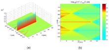
Figure 1: (a) 3D field-intensity of the resulting beam. (b) Orthogonal projection of the resulting beam in logaritmic scale.

3 Electromagnetic beams: The paraxial regime

It should be clear to the reader that the present method is exact, i.e., the obtained beams (with the desired LIPs) in absorbing media are exact solutions to the scalar wave equation and can possess transverse spots of any sizes, from wavelength dimensions to infinity.

In spite of the method has been developed to scalar fields, it can be used in electromagnetism (optics, microwaves, etc..) in the paraxial regime, where the scalar beam $\Psi$ of the previous section would represent the transverse cartesian electric field component of a linearly polarized electromagnetic beam, being $|\Psi|^{2}$ proportional to the time-averaged electromagnetic energy density. In these cases, the beam spot size must be much greater than the correspondent wavelength. This can be done by choosing the parameter $Q$ of Eq.(8) as $Q\approx n_{R}\omega/c$.

We are going to elucidate all these points.

Consider an absorbing, linear, homogeneous and isotropic medium without boundaries and without free charges and free currents.

The electric (and magnetic) field obeys, in the monochromatic case, the Helmholtz equation:

$$\nabla^{2}\mathbf{E}+k^{2}\mathbf{E}\;=\;0$$ (16)

with $\mathbf{E}=\mathcal{E}(x,y,z)e^{-i\omega t}$ and where $k$ is the complex wave number:

$$k\;=\;\omega\sqrt{\mu(\omega)\epsilon(\omega)}\;=\;\omega\sqrt{\mu\left(\epsilon_{b}+i\frac{\sigma}{\omega}\right)}$$ (17)

being $\epsilon_{b}(\omega)$ the electric permittivity due to bound electrons, $\sigma(\omega)$ the electric conductivity and $\mu\approx\mu_{0}$ is the magnetic permeability.

Writing $k$ as

$$k=k_{R}+ik_{I}$$ (18)

and considering the frequency not so close to the resonance regions, we have[29]:

$$k_{R}\approx\omega\sqrt{\frac{\mu_{0}\epsilon_{b}}{2}}\left[\sqrt{1+\left(\frac{\sigma}{\epsilon_{b}\omega}\right)^{2}}\,+1\right]^{1/2}$$ (19)

$$k_{I}\approx\omega\sqrt{\frac{\mu_{0}\epsilon_{b}}{2}}\left[\sqrt{1+\left(\frac{\sigma}{\epsilon_{b}\omega}\right)^{2}}\,-1\right]^{1/2}$$ (20)

with the absorption coefficient $\alpha=2k_{I}$.

Let $\mathbf{E}$ be an electric field given by:

$$\mathbf{E}\;=\;E_{x}\,\mathbf{e}_{x}+E_{z}\,\mathbf{e}_{z}\,\,,$$ (21)

and let us apply our scalar method to the cartesian component $E_{x}$:

$$\begin{array}[]{clr}E_{x}(\rho,z,t)&\;=\;\displaystyle{e^{-i\,\omega\,t}\,\sum_{m=-N}^{N}A_{m}\,J_{0}(k_{\rho\,m}\,\rho)\,e^{i\beta_{m}z}}\\ \\ &\;=\;\displaystyle{e^{-i\,\omega\,t}\,e^{i\,Q\,z}\,\sum_{m=-N}^{N}A_{m}\,J_{0}((k_{\rho R_{m}}+ik_{\rho I_{m}})\,\rho)\,e^{-\beta_{I_{m}}z}\,e^{i\,\frac{2\pi}{L}m\,z}}\,\,,\end{array}$$ (22)

where, as before, $\beta_{m}=\beta_{R_{m}}+i\beta_{I_{m}}$ and $k_{\rho m}=k_{\rho R_{m}}+ik_{\rho I_{m}}$ are chosen according to the Eqs.(8,9,11,6), and $A_{m}$ calculated through Eq.(13), being $|F(z)|^{2}$ the desired LIP to the electric field component $E_{x}$.

Now, to satisfy the Gauss law $\nabla\cdot\mathbf{D}=0$ (no free charges), with $\mathbf{E}=E_{x}\,\mathbf{e}_{x}+E_{z}\,\mathbf{e}_{z}$, in the monochromatic regime, we must have:

$$E_{z}\;=\;-\int\frac{\partial E_{x}}{\partial x}dz$$ (23)

Using $E_{x}$ as giving by Eq.(22), we found:

$$E_{z}(\rho,\phi,z,t)\;=\;\displaystyle{e^{-i\,\omega\,t}\,\sum_{m=-N}^{N}A_{m}\,\frac{k_{\rho m}}{\beta_{m}}\,J_{1}(k_{\rho\,m}\,\rho)\,\cos\phi\,e^{i\beta_{m}z}}$$ (24)

The paraxial regime is characterized by beams whose wave vectors of their constituent plane waves are almost parallel to their propagation directions. In our case, this direction is “$+z$” and the paraxial regime is reached by putting $Q\approx n_{R}\omega/c$, implicating that $|k_{\rho m}/\beta_{m}|<<1$, which in turn implicates that $|E_{z}|<<|E_{x}|$. So, in this circumstance, we can use the so called paraxial approximation and write the electric field (21) as

$$\mathbf{E}\approx E_{x}\,\mathbf{e}_{x}\;=\;\left(\displaystyle{e^{-i\,\omega\,t}\,\sum_{m=-N}^{N}A_{m}\,J_{0}(k_{\rho\,m}\,\rho)\,e^{i\beta_{m}z}}\right)\mathbf{e}_{x}\,\,,$$ (25)

(paraxial approximation)

The associated magnetic field can be found through Faraday’s law:

$$\mathbf{B}\;=\;-\,\frac{i}{\omega}\,\nabla\times\mathbf{E}$$ (26)

Considering the electric field given by (21,22,24), it is easy to show that in the paraxial regime the above expression can be approximated as

$$\mathbf{B}\,\approx\,\displaystyle{-\frac{i}{\omega}\frac{\partial E_{x}}{\partial z}}\mathbf{e}_{y}\;=\;\left(\displaystyle{e^{-i\,\omega\,t}\,\sum_{m=-N}^{N}A_{m}\,\frac{\beta_{m}}{\omega}\,J_{0}(k_{\rho\,m}\,\rho)\,e^{i\beta_{m}z}}\right)\mathbf{e}_{y}$$ (27)

(paraxial approximation)

Remembering that $\beta_{m}=\beta_{R_{m}}+i\beta_{I_{m}}=\beta_{R_{m}}+i(n_{I}/n_{R})\beta_{R_{m}}$, and that $0\leq\beta_{R_{m}}\leq Q+2\pi m/L$, the paraxial regime ($Q\approx n_{R}\omega/c$) implies that $\beta_{R_{m}}\approx n_{R}\omega/c$, and in this case $\beta_{m}/\omega\approx n/c\,$ (where $n=n_{r}+in_{I}$ is the complex refractive index). So, we can make another approximation in Eq.(27) writing:

$$\mathbf{B}\,\approx\,\frac{n}{c}\left(\displaystyle{e^{-i\,\omega\,t}\,\sum_{m=-N}^{N}A_{m}\,J_{0}(k_{\rho\,m}\,\rho)\,e^{i\beta_{m}z}}\right)\mathbf{e}_{y}$$ (28)

or

$$\mathbf{B}\,\approx\,\frac{n}{c}\mathbf{e}_{z}\times\mathbf{E}\;=\;\frac{n}{c}E_{x}\mathbf{e}_{y}$$ (29)

(paraxial approximation)

Using Eqs.(25,29), we immediately see that the time-averaged energy density for monochromatic electromagnetic fields, $u=(1/4)\rm{Re}(\mathbf{E}\cdot\mathbf{D}^{*}+\mathbf{B}\cdot\mathbf{H}^{*})$, can be approximated as

$$u\,\approx\,\frac{1}{4}\rm{Re}\left(\epsilon^{*}+\frac{|n|^{2}}{\mu^{*}c^{2}}\right)|E_{x}|^{2}\propto|E_{x}|^{2}$$ (30)

(paraxial approximation)

So, we can use our scalar method to obtain, in absorbing media, paraxial electromagnetic beams whose the time-averaged energy densities on the propagation axis can assume any desired patterns within an interval $0\leq z\leq L$.

4 Extending the method to nonaxially symmetric beams: Increasing the control over the transverse intensity pattern.

The method developed in [3] allows a strong control over the LIP (on $\rho=0$) of beams propagating in absorbing media.

Once we have controlled the beam’s LIP, the transverse intensity pattern (TIP) can be shaped in a limited way; more specifically, the spot size of the resultant beam can be chosen by a suitable choice of the parameter $Q$ via Eq.(14).

In this section we are going to show that it is possible to get a more efficient control over the TIP, maintaining, at same time, a strong control over the LIP. It will be possible, for instance, to shift the desired LIP from $\rho=0$ to $\rho=\rho^{\prime}>0$. In other words, we will be able to construct the desired LIP over cylindrical surfaces (instead of over the line $\rho=0$). Below we explain this new procedure.

To obtain these new beams we proceed as before, choosing the desired LIP on $\rho=0$ within $0\leq z\leq L$, choosing the values of $Q$ and $N$ (observing the Eq.(9)), and calculating the values of $A_{m}$ through Eq.(13).

Having done this, we replace the zero order Bessel beams in superposition (10) with higher order ones. The new beam is written as:

$${\Psi(\rho,\phi,z,t)\;=\;e^{-i\,\omega\,t}\,e^{i\,Q\,z}\,e^{i\,\mu\,\phi}\,\sum_{m=-N}^{N}A_{m}\,J_{\mu}(k_{\rho\,m}\,\rho)\,e^{-\beta_{I_{m}}z}\,e^{i\,\frac{2\pi}{L}m\,z}}\;,$$ (31)

with $\mu$ a positive integer and all other parameters ($Q$, $N$, $L$ and $A_{m}$) given and calculated as before.

For the situations considered here, we have that $n_{I}<<n_{R}\rightarrow k_{\rho I_{m}}<<k_{\rho R_{m}}$. This implies that for each mth Bessel function in Eq.(10) is valid: $J_{\mu}[(k_{\rho R_{m}}+ik_{\rho I_{m}})\rho]\approx J_{\mu}(k_{\rho R_{m}}\rho)$ for $0<\rho<<1/k_{\rho I_{m}}$, and in this range each mth Bessel function reaches its maximum value at $\rho=\rho^{\prime}_{m}$, being $\rho^{\prime}_{m}$ the first positive root of the equation $({\rm d}\,J_{\mu}(k_{\rho R_{m}}\rho)/{\rm d}\rho)|_{\rho^{\prime}_{m}}=0$.

The values of $\rho^{\prime}_{m}$ are located around the central value $\rho^{\prime}_{m=0}$ and we can expect a shift of the desired LIP from $\rho=0$ to $\rho\approx\rho^{\prime}_{m=0}$.

We have confirmed that conjecture in all situations considered by us, mainly in the cases where there is no considerable difference among the values of $k_{\rho R_{m}}$.

With this extension of the original method, it is possible to model the LIP over cylindrical surfaces, obtaining very interesting static configuration of the field intensity. In particular, we can construct (in absorbing media) hollow beams resistant to the attenuation and diffraction effects.

To show this method working we are going to obtain a cylindrical light surface of constant intensity in an absorbing medium with $n_{R}=1.5$ and $\alpha=20{\rm m}^{-1}$ (at $\lambda=308$nm $\rightarrow$ $\omega=6.12\times 10^{15}$Hz), which implies that $n_{I}=0.49\times 10^{-6}$. At this angular frequency, an ordinary beam would possess a depth of penetration of $5\,$cm in this medium.

Let us choose, within $0\leq z\leq L$, a LIP as that of section 1, Eq.(15):

$$F(z)\;=\;\left\{\begin{array}[]{clr}&1\;\;\;{\rm for}\;\;\;0\leq z\leq Z\\ &0\;\;\;\mbox{elsewhere},\end{array}\right.$$ (32)

being $Z=25\;$cm and $L=33\;$cm.

As in section 1, we put $Q=0.9999n_{R}\omega/c$ in Eq.(8). With the chosen values to $Q$ and $L$, the maximum value allowed to $N$ is $N=154$, but for simplicity reasons we choose $N=20$.

Using equations(8,9,11,6,13) we evaluate all the $\beta_{m}$, $k_{\rho m}$ and $A_{m}$. But, as we have explained in this section, instead of using all these values in (10), we use them in the superposition (31), where we choose $\mu=4$.

According to the previous discussion, we can expect the desired LIP over a cylindrical surface of radius $\rho\approx 5,318/k_{\rho R_{m=0}}=12.289\,\mu$m (that is where the function $J_{4}(k_{\rho R_{m=0}}\rho)$ assumes its maximum value).

We can see in figure(2.a) the resulting intensity field in a three-dimensional pattern. Its orthogonal projection shown in Fig.(2.b) clearly confirms the cylindrical surface of light intensity. Figure (2.c) depicts the transverse intensity pattern at $z=L/2$. It is possible to note that the transverse peak intensity is located at $\rho=12.285\,\mu$m, a value near to the predicted one.

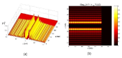
Figure 2: (a) 3D field-intensity of the resulting beam. (b) Its orthogonal projection.

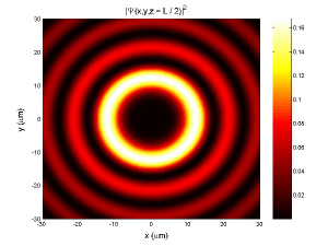
Figure 3: The beam’s transverse intensity pattern at $z=L/2$

This interesting field configuration is resistant to the attenuation and diffraction effects till the distance $z=25$cm. We should remember that any other ordinary beam at the same frequency, propagating in the same medium, would have a penetration depth of only $5$cm.

5 Finite aperture generation of the diffraction-attenuation resistant beams

As we have seen, the solution (5), with (8,9,11,6,13), represents propagating beams in absorbing media with the remarkable characteristic of allowing us to choose the desired LIP on $\rho=0$, within $0\leq z\leq L$, being the spot sizes regulated by the value of the parameter $Q$. The same occurs with solution (31), which in turn allows us to choose the desired LIP on a cylindrical surface.

Now, we must remember that, in spite of the beams (5) and (31) be exact solutions, they do not represent beams generated or truncated by finite apertures. Actually, fields given by those solutions in all points of space would require infinite apertures to be generated.

However, if a Bessel beam given by Eq.(2) is truncated by a finite aperture of radius $R>>2.4/k_{\rho R}$ situated on the plane $z=0$, the radiated field – in the spatial region $0<z<R/\tan\theta\equiv Z$ (the diffractionless distance of a truncated Bessel beam) and $0\leq\rho\leq(1-z/Z)R\,$ – can be approximately described[2, 3, 6] by Eq.(2).

Taking into account that the solution (10) is a linear superposition of Bessel beams, we can expect that when it is truncated by a finite aperture of radius $R>>2.4/k_{\rho R_{m=N}}$, the radiated field – in the region $0<z<R/\tan\theta_{m=-N}\equiv Z_{m=-N}$ and $0\leq\rho\leq(1-z/Z_{m=-N})R\,$ – will be approximately given by Eq.(10).

Now, as we are interested in controlling the LIP of the truncated beam within $0\leq z\leq L$ , we have to guarantee that, after the truncation, all Bessel beams in (10) maintain their characteristics until $z=L$. This is possible if both conditions are satisfied:

$$R>>\frac{2.4}{k_{\rho R_{m=N}}}$$ (33)

and

$$Z_{m=-N}>L\,\,\rightarrow\,\,\frac{R}{\tan\theta_{m=-N}}>L\,\,\rightarrow\,\,R>L\sqrt{\frac{n_{R}^{2}}{c^{2}}\frac{\omega^{2}}{\beta_{R_{m=-N}}^{2}}-1}$$ (34)

So we can expect that by choosing a finite aperture of radius $R$ large enough to satisfy (33) and (34), the truncated versions of the diffraction attenuation resistant beams will maintain their characteristics, i.e., we will continue to be able to control the beam’s LIP.

In order to confirm our expectation, some examples shall be presented, where we choose some desired LIPs and obtain the correspondent ideal beam solutions, $\Psi(\rho,\phi,z,t)$, through Eqs.(5,8,9,11,6,13). These ideal solutions, in turn, are used for obtaining their truncated versions, $\Psi_{T}(\rho,\phi,z,t)$, through numerical calculation of the Rayleigh-Sommerfeld diffraction integral for monochromatic waves[30]:

$$\Psi_{T}(\rho,\phi,z,t)\;=\;\frac{1}{2\pi}\int_{0}^{2\pi}d\phi^{\prime}\int_{0}^{R}d\rho^{\prime}\,\rho^{\prime}\,\frac{e^{ikD}}{D}\left(\frac{\partial}{\partial z^{\prime}}\,\Psi(\rho^{\prime},\phi^{\prime},z^{\prime},t)\right)_{z^{\prime}=0}\,\,\,,$$ (35)

where a circular aperture of radius $R$, on the plane $z^{\prime}=0$, is used for the truncation, being the distance $D=\sqrt{\left(z-z^{\prime}\right)^{2}+\rho^{2}+\rho^{\prime 2}-2\rho\rho^{\prime}\cos\left(\phi-\phi^{\prime}\right)}$ the separation between the source and observation points.

A. First Example

Here we are going to calculate numerically the truncated version of the ideal diffraction-attenuation resistant beam obtained in the example of Section II and in ref.[3].

The medium in question has refractive index $n=n_{R}+in_{I}=1.5+i\,0.49\times 10^{-6}$ in $\lambda=308{\rm nm}$ (i.e., $\omega=6.12\times 10^{15}$Hz). The ideal beam in that example was constructed to possess (in $\omega=6.12\times 10^{15}$Hz) a spot radius $\Delta\rho=5.6\,\mu$m and a constant intensity of its central spot until a distance of $25\,$cm. These characteristics were reached through the fundamental ideal solution (10), with Eqs.(8,9,11,6,13), by choosing the desired LIP $|F(z)|^{2}$ (on $\rho=0$), within $0\leq z\leq L$, according to Eq.(15), putting $Z=25\;$cm and $L=33\;$cm. The values of $Q$ and $N$ were chosen to be $0.9999n_{R}\omega/c$ and $20$ respectively.

This ideal beam solution is used as the aperture excitation, $\Psi(\rho^{\prime},z^{\prime},t)$, in the Rayleigh-Sommerfeld diffraction integral, Eq.(35), which is numerically calculated to yield $\Psi_{T}(\rho,z,t)$, i.e., the truncated version of this beam.

According to our above discussion, the truncated beam shall possesses a behavior very similar to the ideal one provided that the aperture radius $R$ satisfy both conditions (33, 34), which furnishes in this case $R\geq 4.9\,$mm. However, due to the fact that the chosen on-axis LIP has null value within $Z<z<L$, we can replace $L$ in condition (34) with $Z$, obtaining in this case $R\geq 3.8\,$mm. We choose $R=3.8\,$mm.

After numerical calculation of (35), we obtain the result plotted below. Comparing Figure(3) with Figure(1a) of the ideal beam of Section II, we can see that our expectations were correct, i.e., by choosing an aperture radius big enough, the truncated version becomes very close to the ideal solution in the spatial region of interest.

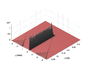
Figure 4: The truncated version of the ideal diffraction-attenuation resistant beam obtained in the example of Section II

B. Second Example

In [3] one of the authors obtained, in an absorbing media, an ideal (i.e., not truncated) beam presenting an interesting and counterintuitive characteristic. There, it was considered a medium with refractive index $n=n_{R}+in_{I}=1.5+i0.46\times 10^{-6}$ (which implies in a penetration depth of $5\,$cm) at $\omega=6.12\times 10^{15}\,$Hz. At this angular frequency an ideal beam was shaped to possess a spot radius $\Delta\rho=5.6\,\mu$m and a modest exponential growth of its intensity until a distance of $25\,$cm, suffering after this a strong intensity fall.

In order to reach these characteristics, the desired on axis LIP, $|F(z)|^{2}$, within $0\leq z\leq L$, was chosen according to:

$$F(z)\;=\;\left\{\begin{array}[]{clr}&{\rm exp}(z/Z)\;\;\;{\rm for}\;\;\;0\leq z\leq Z\\ &0\;\;\;\mbox{elsewhere},\end{array}\right.$$ (36)

with $Z=25\,$cm and $L=33\;$cm. Taking into account Eq.(14), it was chosen $Q=0.9999n_{R}\omega/c$ and the value of $N$ was chosen to be $N=20$.

With this, the (ideal) desired beam, $\Psi(\rho,z,t)$, was obtained in [3] through the fundamental solution (10), with Eqs.(8,9,11,6,13). Below we plotted this resulting ideal (i.e., not truncated) beam.

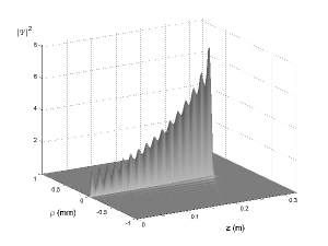
Figure 5: Ideal beam presenting a moderate exponential growth in an absorbing medium

In this example, we are going to use Eq.(35) to obtain the truncated version, $\Psi_{T}(\rho,z,t)$, of the above ideal beam.

By using conditions (33, 34) for an efficient finite aperture generation, we obtain that the aperture radius should obey $R\geq 4.9\,$mm. But, for the same reason of the previous example, we can adopt $R\geq 3.8\,$mm, and we choose $R=3.8\,$mm.

The numerical calculation of Eq.(35) yields the truncated beam plotted below:

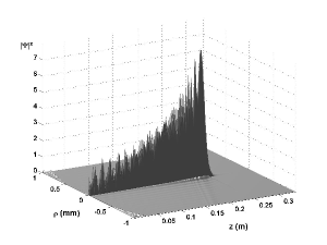
Figure 6: Truncated version of the beam with exponential growth

We can see an excellent agreement between the ideal beam and the truncated one in the region of interest, confirming that the method works very well in more realistic situations close to the experimental ones.

6 Conclusions

A few years ago[3] it was developed an interesting theoretical method, from which it is possible to construct, in absorbing media, axially symmetric beams whose the LIP can be previously chosen. As a particular case, diffraction-attenuation resistant beams were obtained, that is, beams capable of maintaining both, the size and the intensity of their central spots.

In this paper we elucidate how to apply this scalar method in paraxial electromagnetic waves and extended it to include non-axially symmetric beams, allowing in this way, besides the strong control over the longitudinal intensity patter, a certain control over the transverse one. With this extension, it is possible to model the LIP over cylindrical surfaces. In particular, we can construct (in absorbing media) hollow beams resistant to the attenuation and diffraction effects.

We also use the Rayleigh-Sommerfeld diffraction integral to obtain the truncated versions of these new beams, verifying that, provided that the aperture used for truncation is big enough, the truncated beams possess the same interesting characteristics of the ideal beams. This verification is important because it confirms that the method works very well in more realistic situations close to the experimental ones.

These new beams can possess potential applications, such as free space optics, medical apparatuses, remote sensing, etc..

References

- [1] M.Zamboni-Rached, “Stationary optical wave fields with arbitrary longitudinal shape by superposing equal frequency Bessel beams: Frozen Waves ”, Optics Express, vol.12, pp.4001-4006 (2004).
- [2] M.Zamboni-Rached, E.Recami and H.E.Hernández-Figueroa, “Theory of Frozen Waves: Modelling the Shape of Stationary Wave Fields ”, Journal of the Optical Society of America A 11, pp.2465-2475 (2005).
- [3] M.Zamboni-Rached, “Diffraction-Attenuation resistant beams in absorbing media”, Opt. Express 14, pp.1804-1809 (2006).
- [4] See Localized Waves: Theory and Applications, ed. by H.E.Hernández-Figueroa, M.Zamboni-Rached, and E.Recami (J.Wiley; New York, Jan.2008), book, 369 pages; and refs. therein.
- [5] C. J. R. Sheppard and T. Wilson, “Gaussian-beam theory of lenses with annular aperture”, IEE Journal on Microwaves, Optics and Acoustics, 2, 105-112 (1978).
- [6] J. Durnin, J. J. Miceli and J. H. Eberly, “Diffraction-free beams,” Physical Review Letters 58, 1499-1501 (1987).
- [7] I. M. Besieris, A. M. Shaarawi and R. W. Ziolkowski, “A bi-directional traveling plane wave representation of exact solutions of the scalar wave equation,” J. Math. Phys. 30, 1254-1269 (1989).
- [8] R. W. Ziolkowski, I. M. Besieris and A. M. Shaarawi, “Aperture realizations of exact solutions to homogeneous-wave equations,” J. Opt. Soc. Am. A 10, 75-87 (1993).
- [9] J.-Y. Lu and J. F. Greenleaf,“Nondiffracting X-waves: Exact solutions to free-space scalar wave equation and their finite aperture realizations,” IEEE Trans.Ultrason. Ferroelectr. Freq. Control 39, 19-31 (1992).
- [10] E. Recami, “On localized X-shaped Superluminal solutions to Maxwell equations”, Physica A 252, 586-610 (1998).
- [11] P. Saari and K. Reivelt, “Evidence of X-shaped propagation-invariant localized light waves,” Phys. Rev. Lett. 79, 4135-4138 (1997).
- [12] D. Mugnai, A. Ranfagni and R. Ruggeri, “Observation of superluminal behaviors in wave propagation,” Phys. Rev. Lett. 84, 4830-4833 (2000). This paper aroused some criticisms, to which the authors replied.
- [13] See, e.g., M. Zamboni-Rached, E. Recami and H. E. Hernández-Figueroa, “New localized Superluminal solutions to the wave equations with finite total energies and arbitrary frequencies,” European Physical Journal D 21, 217-228 (2002).
- [14] M. Zamboni-Rached, K. Z. Nóbrega, C. A. Dartora, and H. E. Hernández-Figueroa, “On the localized superluminal solutions to the Maxwell equations,” IEEE Journal of Selected Topics in Quantum Electronics 9, 59-73 (2003), and refs. therein.
- [15] C. Conti, S. Trillo, G. Valiulis, A. Piskarskas, O. Jedrkiewicz, J. Trull, and P. Di Trapani, “Nonlinear electromagnetic x-waves”, Phys. Rev. Lett., 90:170406 (2003).
- [16] M. Zamboni-Rached and H. E. Hernández-Figueroa, “A rigorous analysis of localized wave propagation in optical fibers”, Opt. Commun., 191, 49-54 (2001).
- [17] M. Zamboni-Rached, E. Recami, and F. Fontana, “Localized Superluminal solutions to Maxwell equations propagating along a normal-sized waveguide”, Phys. Rev., E, 64, 066603 (2001).
- [18] M. Zamboni-Rached, K. Z. Nóbrega, E. Recami and H. E. Hernandez F., “Superluminal X-shaped beams propagating without distortion along a coaxial guide”, Phys. Rev., E, 66, 046617 (2002).
- [19] M. Zamboni-Rached, F. Fontana and E. Recami, “Superluminal localized solutions to Maxwell equations propagating along a waveguide: The finite-energy case”, Phys. Rev., E, 67, 036620 (2003).
- [20] M. Zamboni-Rached, K. Z. Nóbrega, H. E. Hernández-Figueroa, and E. Recami, “Localized Superluminal solutions to the wave equation in (vacuum or) dispersive media, for arbitrary frequencies and with adjustable bandwidth”, Optics Communications, 226, 15-23 (2003).
- [21] S. Longhi and D. Janner, “X-shaped waves in photonic crystals”, Phys. Rev. B, 70, 235123 (2004).
- [22] M. Zamboni-Rached and E. Recami, “Subluminal wave bullets: Exact localized subluminal solutions to the wave equations,” Phys. Rev. A, Vol. 77, 033824 (2008).
- [23] M. A. Porras, R. Borghi, and M. Santarsiero, “Suppression of dispersion broadening of light pulses with Bessel-Gauss beams”, Optics Communications, 206, 235-241 (2003).
- [24] M. Zamboni-Rached, H. E. Hernández-Figueroa e E. Recami, “Chirped optical X-shaped pulses in material media,” J. Opt. Soc. Am., A, 21, 2455-2463 (2004).
- [25] Z. Bouchal and J. Wagner, “Self-reconstruction effect in free propagation wavefield,” Optics Communications 176, 299-307 (2000).
- [26] M. Zamboni-Rached, A. Shaarawi and E. Recami, “Focused X-shaped pulses,” Journal of the Optical Society of America A 21, 1564-1574 (2004); and refs. therein.
- [27] Colin J. R. Sheppard and Peeter Saari, “Lommel pulses: An analytic form for localized waves of the focus wave mode type with bandlimited spectrum”, Optics Express, 16, 150-160 (2008).
- [28] M. Zamboni-Rached, “Unidirectional decomposition method for obtaining exact localized wave solutions totally free of backward components”, Physical Review A, Vol. 79, 013816 (2009).
- [29] J. D. Jackson: Classical Electrodynamics (J.Wiley; NJ, 1998).
- [30] J.W.Goodman: Introduction to Fourier Optics (McGraw Hill College; San Francisco, 1968).