Interactions in quantum fluids

Part I First part

First part

Chapter 0 Interactions in quantum fluids

1 Introduction

The problem of interacting quantum particles is one of the most fascinating problems in physics, with an history nearly as long as quantum mechanics itself. From a pure fundamental point of view this is a staggering problem. Even in a one gram of solid there are more particles interacting together than there are stars in the universe. In addition these particles behave as waves, since quantum effects are important and must obey symmetrization or anti-symmetrization principles. It it thus no wonder that despite nearly one century of efforts we still lack the tools to give a complete solution of this problem, and that sometimes even the concepts needed to describe such interacting systems need to be sharpened.

The problem is not simply an academic one however. Indeed with the discovery of quantum mechanics, came the understanding of the behavior of electrons in solids and the band structure theory. One of the fantastic success of such a theory was to understand why some materials are metals, insulators or semiconductors, an understanding which is at the root of the discovery of the transistor and all the modern electronic industry. An additional piece of knowledge was added by Landau, with the so called Fermi liquid theory, where he showed that in most fermionic systems the effects of interactions could be essentially forgotten, and hidden in the redefinition of simple parameters such as the mass of the particles. Being able to forget about interactions paved the way to study the effects on the real electronic systems of much smaller perturbations than the electron-electron interactions, for example the electron and lattice vibrations. This is at the root of the understanding of many possible orders of the solids, such as superconductivity and magnetism, or the interplay of magnetism and conducting properties of the systems such as the giant magnetoresistance. These properties have also had a profound impact on our everyday’s life.

Now such systems have been intensively studied and the forefront of research has moved to materials for which we cannot hide the effects of interactions anymore. This include in particular the wide class of materials such as the oxides that have properties as varied as being the best superconductors known to date, or exhibit properties such as ferroelectricity. These compounds or others that remain to be discovered are clearly those who will be the materials of the future for applications, and mastering of their properties requires the deep understanding of the effects of interactions. In addition to problems in condensed matter, cold atomic gases have provided recently for marvellous realizations of such strongly correlated systems and have thus added both to the challenge we have to face, but also provided model systems that could help us to make progress in that difficult field.

In these notes I review the basic concepts of the effects of interactions on quantum particles. I focuss here mostly on the case of fermions, but several aspects of interacting bosons will be mentioned as well. The course has been voluntarily kept at an elementary level and should be suitable for students wanting to enter this field. I review the concept of Fermi liquid, and then move to a description of the interaction effects, as well as the main models that are used to tackle these questions. Finally I study the case of one dimensional interacting particles that constitutes a fascinating special case.

2 Fermi liquids

This section is based on a master course given at the university of Geneva, over several years together with C. Berthod, A. Iucci, P. Chudzinski. Many more details can be found on the course notes on http://dpmc.unige.ch/gr_giamarchi/.

1 Weakly interacting fermions

Let me start by recalling briefly some well known but important facts about non interacting fermions. I will not recall the calculation since they can be found in every textbook on solid state physics [Ashcroft and Mermin (1976), Ziman (1972)], but just give the main results. These will be important for the case of interacting electrons.

We consider independent electrons described by the Hamiltonian

$$H_{\rm kin}=\sum_{\vec{k}\sigma}\varepsilon(\vec{k})c^{\dagger}_{\vec{k}\sigma}c_{\vec{k}\sigma}$$ (1)

where the sum over $\vec{k}$ runs in general over the first Brillouin zone. One usually incorporates the chemical potential in the energy $\xi(\vec{k})=\varepsilon(\vec{k})-E_{\text{F}}$ to make sure that $\xi(\vec{k})=0$ at the Fermi level. The ground state of such system is the unpolarized Fermi sea

$$\left|\text{F}\right\rangle=\prod_{\vec{k},\xi(\vec{k})\leq 0}c^{\dagger}_{\vec{k}\uparrow}c^{\dagger}_{k\downarrow}\left|\varnothing\right\rangle$$ (2)

At finite temperature states are occupied with a probability

$$n(k)=\langle c^{\dagger}_{\vec{k}}c_{\vec{k}}\rangle=f_{\text{F}}(\xi(\vec{k}))=\frac{1}{e^{\beta\xi(\vec{k})}+1}$$ (3)

given by the Fermi factor. A very important point, true for most solids, is that the order of magnitude of the Fermi energy is $E_{\text{F}}\sim 1eV\sim 12000K$. This means that the temperature, or most of the energies that are relevant for a solid (for example $30GHz\sim 1K$) are extremely small compared to the Fermi energy. As a result the broadening of the Fermi distribution is extremely small. The important states are thus be the ones in a tiny shell close to the Fermi level, as shown in Fig. 1.

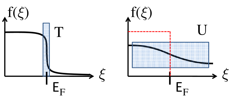
Figure 1: (left) Broadening of the Fermi distribution due to the temperature $T$. Because in most solids the temperature $T$ is much smaller than the Fermi energy $E_{\text{F}}$ only a tiny fraction close to the Fermi level can be excited. These fermions control all the properties of the system. (right) If the interaction $U$ was acting as a temperature and was broadening the Fermi distribution one would get an extremely large broadening. All the consequences of the sharp Fermi distribution (specific heat linear in temperature, compressibility and spin susceptibility going to a constant at low temperatures) would be lost.

The other excitations are completely blocked by the Pauli principle. This hierarchy of energies is of course what confers to fermions in solids their unique properties and make them so different from a classical system. As a consequences some of the response of such a fermion gas are rather unique. The specific heat is linear with temperature (contrarily to the case of a classical gas for which it would be a constant)

$$C_{V}(T)\propto k_{\text{B}}^{2}\mathcal{N}(E_{\text{F}})T$$ (4)

where $\mathcal{N}(E_{\text{F}})$ is the density of states at the Fermi level, and $k_{\text{B}}$ the Boltzmann constant. The compressibility of the fermion gas goes to a constant in the limit $T\to 0$, and the same goes for the spin susceptibility, namely the magnetization $M$ of the electron gas in response to an applied magnetic field $H$

$$\chi=\left(\frac{dM}{dH}\right)_{T}$$ (5)

Note that a system made of independent spins would have had a divergent spin susceptibility when $T\to 0$ instead of a constant one. The slope of the specific heat, the compressibility and the spin susceptibility of the free fermion gas are all controlled, by the same quantity namely the density of states at the Fermi level.

One could thus wonder what would be the effects of interactions on such a behavior. Because of the interactions, the energy of a particle can now fluctuate since the particle can give of take energy from the others. Thus one could naively imagine that the interactions produce an effect on the distribution function similar to the one of a thermal bath, with an effective “temperature” of the order of the strength of the interaction. In order to determine the consequences of such a broadening, one needs to estimate the strength of the interactions. In a solid the interaction is mostly the Coulomb interaction. However, in a metal this interaction is screened beyond a length $\lambda$ that one can easily compute in the Thomas-Fermi approximation [Ashcroft and Mermin (1976), Ziman (1972)]

$$\lambda^{-2}=\frac{e^{2}\mathcal{N}(E_{\text{F}})}{\epsilon_{0}}$$ (6)

where $e$ is the charge of the particles and $\epsilon_{0}$ the dielectric constant of the vacuum. To estimate $\lambda$ we can use the fine structure constant

$$\alpha=\frac{e^{2}}{4\pi\epsilon_{0}\hbar c}=\frac{1}{137}$$ (7)

to obtain

$$\lambda^{-2}=4\pi\alpha\hbar c\mathcal{N}(E_{\text{F}})=4\pi\alpha\hbar c\frac{3n}{2E_{\text{F}}}$$ (8)

where $n$ is the density of particles. Using the density of states per unit volume of free fermions in three dimensions

$$n(\varepsilon)=\frac{m}{2\pi^{2}\hbar^{2}}\left(\frac{2mE_{\text{F}}}{\hbar^{2}}\right)^{1/2}=\frac{3}{2}\frac{n}{E_{\text{F}}}$$ (9)

and $E_{\text{F}}=\hbar v_{\text{F}}k_{\text{F}}$, and $6\pi^{2}n=k_{\text{F}}^{3}$ one gets

$$\lambda^{-2}=\frac{1}{\pi}\alpha\frac{c}{v_{\text{F}}}k_{\text{F}}^{2}$$ (10)

Since $c/v_{\text{F}}\sim 10^{2}$ in most systems, one finds that $k_{\text{F}}\lambda\sim 1$. The screening length is of the order of the inverse Fermi length, i.e. essentially the lattice spacing in normal metals. This is a striking result: not only the Coulomb interaction is screened, but the screening is so efficient that the interaction is practically local. We will use extensively this fact in the definition of models below. Let us now estimate the order of magnitude of this screened interaction. The interaction between two particles can be written as

$$H_{\text{int}}=\int d\vec{r}d\vec{r}^{\prime}V(\vec{r}-\vec{r}^{\prime})\rho(\vec{r})\rho(\vec{r}^{\prime})$$ (11)

Since the interaction is screened it is convenient to replace it by a local interaction. Given our previous result let us simply replace the screening length by $a$ the fermion-fermion distance. The effective potential seen at point $\vec{r}$ by one particle is

$$\int d\vec{r}^{\prime}V(\vec{r}-\vec{r}^{\prime})\rho(\vec{r}^{\prime})$$ (12)

Due to screening we should only integrate within a radius $a$ around the point $r$. Assuming that the density is roughly constant one obtains

$$\int_{|\vec{r}-\vec{r}^{\prime}|<a}d\vec{r}\frac{e^{2}}{4\pi\epsilon_{0}|\vec{r}-\vec{r}^{\prime}|}\rho_{0}\sim\frac{e^{2}\rho_{0}S_{d}a^{d-1}}{4(d-1)\pi\epsilon_{0}}$$ (13)

where $S_{d}$ is the surface of the sphere in $d$ dimensions. Using $\rho_{0}\sim 1/a^{d}$ and (7) one gets

$$\frac{S_{d}\alpha\hbar c}{(d-1)a}$$ (14)

This potential acting on a particle has to be compared with the kinetic energy of this particle at the Fermi level which is $E_{\text{F}}=\hbar v_{\text{F}}k_{\text{F}}$. Since $k_{\text{F}}\sim a^{-1}$ one has again to compare $\alpha$ and $c/v_{\text{F}}$. The two are about the same order of magnitude. The Coulomb energy, even if screened (i.e. even in a very good metal), is thus of the same order of magnitude than the kinetic energy. This means, for solids, typical energies of the order of the electron volt. If such an interaction was acting as a temperature in smearing the Fermi function this would lead to an enormous smearing as shown in Fig. 1.

This would be in complete contradiction with data on most of solids. The specific heat in real materials is found to be linear, albeit with a slope different from the naive free electron picture at temperatures much smaller than the scale of the interactions (see e..g Fig. 1.8 in [Ashcroft and Mermin (1976)]). This would be totally impossible if the interactions had smeared the Fermi distribution to a practically flat distribution. Similarly spin susceptibility and compressibility are still found, e.g. in ³He to be essentially constant at low temperature[Greywall (1983), Greywall (1984)], again implying that the Fermi distribution must remain quite sharp.

In addition, a remarkable experimental technique to look at the single particle excitations, and momenta distributions is provided by the photoemission technique [Damascelli et al. (2003)]. Pending some hypothesis this technique is a direct measure of the spectral function $A(\vec{k},\omega)$ which is the probability of finding an excitation with the energy $\omega$ and a momentum $\vec{k}$. For free particles $A(\vec{k},\omega)=\delta(\omega-\xi(\vec{k}))$. Naively one would expect that, because an energy of the order of the interaction can be exchanged, these perfect peaks are broadened over an energy of the order of the interaction. As can be seen from Fig. 2

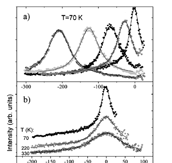
Figure 2: Photoemission data from a Mo (110) surface. (Top) The spectral function $A(\vec{k},\omega)$ is plotted as a function of $\omega$. The zero denotes the Fermi level. Different peaks corresponds to different values of $\vec{k}$. One sees that, contrarily to naive expectations, the peaks in the spectral function become narrower and narrower as one gets closer to the Fermi energy. (Bot) Width of a peak close to the Fermi level as a function of the temperature $T$. One sees that the width of the peak is controlled in a large part by the temperature, which corresponds to energies several order of magnitude smaller than the typical energy of the interactions. [After [Valla et al. (1999)]]

this is clearly not the case. Very sharp peaks exist, and become sharper and sharper as one gets closer to the Fermi energy. The momentum distribution seems to be broadened uniquely by the temperature when one is at the Fermi surface.

One is thus faced with a remarkable puzzle: the “free electron” picture seems, at least qualitatively, to work much better than it should, based on estimates of the interaction strength. This must hide a profound effect, and is thus a great theoretical challenge.

2 Landau Fermi liquid theory

The solution to this puzzle was given by Landau and is known under the name of Fermi liquid theory [Landau (1957a), Landau (1957b)].

Let me first give a very qualitative description of the underlying ideas before embarking on a more rigorous definition and derivation. The main idea behind Fermi liquids [Nozieres (1961)] is to look at the excitations that would exist above the ground state of the system. In the absence of interactions the ground state is the Fermi sea (2). Let us assume now that one turns on the interactions. This ground state will evolve into a very complicated object, that we will be unable to describe, but that does not interest us directly. What we need are the excitations that correspond to the addition or removal (creation of a hole) of a fermion in the ground state. In the absence of interactions one just add an electron in an empty $\vec{k}$ state and such an excitation does not care about the presence of all the other electrons in the ground state (otherwise than via the Pauli principle which prevents from creating it in an already occupied state). In the presence of interactions this will not be the case and the added particle interacts with the existing particles in the ground state. For example for repulsive interactions one can expect that this excitation repels other electrons in its vicinity. This is schematically represented in Fig. 3.

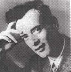
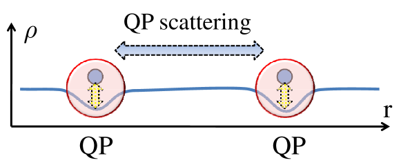
Figure 3: (top) Lev Landau, the man behind the Fermi liquid theory (and many other things). (bot) In a Fermi liquid, the few excitations above the ground state can interact strongly with all the other electrons present in the ground state. The effect of such interactions is strong and lead to a strong change of the parameters compared to free electrons. The combined object behaves as a single particle, named a quasiparticle. The quasiparticles have thus characteristics depending strongly on the interactions. However the scattering of the quasiparticles is blocked by the Pauli principle leaving a very small phase space of scattering. The lifetime of the quasiparticles is thus extremely large. This is the essence of the Fermi liquid theory.

On the other hand if one is at low temperature (compared to the Fermi energy) there are very few of such excitations and one can thus neglect the interactions between them. This picture strongly suggests that the main interaction is between the excitation and the ground state. This defines a new composite object (fermion or hole surrounded by its own polarization cloud). This complex object essentially behaves as a particle, with the same quantum numbers (charge, spin) than the original fermion, albeit with renormalized parameters, for example its mass. This image thus strongly suggests that even in the presence of interactions good excitations looking like free particles, still exists. These particle resemble free fermions but with a renormalized energy $E(\vec{k})$ and thus a renormalized mass. Since the interaction has been incorporated in the definition of such objects, it will not act as a source of broadening for their momentum distribution and the momentum distribution for the quasiparticles will remain very sharp, with only the small temperature broadening.

Of course the above is just a qualitative idea. Let me now give a more formal treatment. For that we can consider the retarded single correlation function [Mahan (1981), Abrikosov et al. (1963)]

$$G(\vec{k},t_{2}-t_{1})=-i\operatorname{\theta}(t_{2}-t_{1})\langle[c_{\vec{k},t_{2}},c^{\dagger}_{\vec{k},t_{1}}]_{+}\rangle$$ (15)

This correlation represents the creation of a particle in a well defined momentum state $\vec{k}$ at time $t_{1}$, let it propagate and then tries to destroy it in a well defined momentum state $\vec{k}$ at time $t_{2}$. It thus measures how well in the interacting system the single particle excitations still resemble plane or Bloch waves, i.e. independent particles. This corresponds to the gedanken experiment described in Fig. 4.

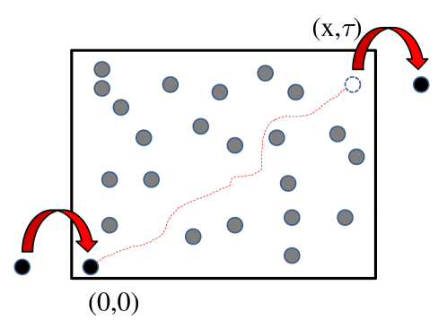
Figure 4: One way to understand the nature of the excitations in an interacting system is to inject a particle at point $r_{1}$ and time $t=0$. The resulting system evolves, and then one destroys a particle at time $t$ and point $r_{2}$. The amplitude of such a process indicates how much the propagation of the excitation between the two points and times is similar to the case of non interacting electrons or not.

The imaginary part of the Fourier transform of this correlation function is just the spectral function

$$A(\vec{k},\omega)=\frac{-1}{\pi}\operatorname{Im}G(\vec{k},\omega)$$ (16)

The spectral function measures the probability to find a single particle excitation with an energy $\omega$ and a momentum $\vec{k}$. It does obey the sum rule of probabilities $\int d\omega A(\vec{k},\omega)=1$. The general form of the retarded correlation is

$$G(\vec{k},\omega)=\frac{1}{\omega-\xi(\vec{k})-\Sigma(\vec{k},\omega)+i\delta}$$ (17)

where $\Sigma(\vec{k},\omega)$, called the self energy, is a certain function of momenta and frequency. The relation (17) defines the function $\Sigma$. For noninteracting systems $\Sigma=0$, and perturbative methods (Feynman diagrams) exist to compute $\Sigma$ in powers of the interaction [Mahan (1981), Abrikosov et al. (1963)]. However we will not attempt here to compute the self energy $\Sigma$ but simply to examine how it controls the spectral function. I incorporate the small imaginary part $i\delta$ in $\Sigma$ for simplicity, since one can expect in general $\Sigma$ to have a finite imaginary part as well. The spectral function is

$$A(\vec{k},\omega)=-\frac{1}{\pi}\frac{\operatorname{Im}\Sigma(\vec{k},\omega)}{(\omega-\xi(\vec{k})-\operatorname{Re}\Sigma(\vec{k},\omega))^{2}+(\operatorname{Im}\Sigma(\vec{k},\omega))^{2}}$$ (18)

We see that $\operatorname{Im}\Sigma$ and $\operatorname{Re}\Sigma$ play very different roles in the spectral function. Note that quite generally (18) imposes that $\operatorname{Im}\Sigma(\vec{k},\omega)<0$ to get a positive spectral function. In the absence of interactions $\Sigma=0$ and one recovers

$$A(\vec{k},\omega)=\delta(\omega-\xi(\vec{k}))$$ (19)

The imaginary part of the self energy gives the broadening of the peaks, which now acquire a lorentzian like form, with a width of order $\operatorname{Im}\Sigma$ and a height or order $1/\operatorname{Im}\Sigma$. This can be readily seen from (18), for example by setting the real part of $\Sigma$ to zero and taking a constant $\operatorname{Im}\Sigma$. Note that now the peaks are not centered around $\xi(\vec{k})$ anymore but have a maximum at a an energy $E(\vec{k})$ which is a solution $\omega=E(\vec{k})$ of

$$\omega-\xi(\vec{k})-\operatorname{Re}\Sigma(\vec{k},\omega)=0$$ (20)

The imaginary part thus defines the broadening of the peaks, i.e. how sharply the excitations are defined, while the real part gives the new energy of the excitations. Let us look at these two elements in slightly more details.

Lifetime:

The imaginary part of the self energy controls the spread in energy of the particles. This leads to the physical image of a particle with an average energy $\omega=E(\vec{k})$, related to its momentum, but with a certain spread $\operatorname{Im}\Sigma$ in energy. To understand the physics of this spread let us consider the Green function of a particle in real time:

$$G(\vec{k},t)=-i\operatorname{\theta}(t)e^{-iE(\vec{k})t}e^{-t/\tau}$$ (21)

The oscillatory part is the normal time evolution of a wavefunction of a particle with an energy $E(\vec{k})$. We have added the exponential decay that would be produced by a finite lifetime $\tau$ for the particle. The Fourier transform becomes

$$G(\vec{k},\omega)=\frac{1}{\omega-E(\vec{k})+i/\tau}$$ (22)

and the spectral function is

$$A(\vec{k},\omega)=\frac{1}{\pi}\frac{1/\tau}{(\omega-E(\vec{k}))^{2}+(1/\tau)^{2}}$$ (23)

which is essentially the one we are considering with the identification

$$\frac{1}{\tau}=\operatorname{Im}\Sigma$$ (24)

We thus see from (21) that a Lorentzian-like spectral function corresponds to a particle with a well defined energy $E(\vec{k})$ which defines the center of the peak, but also with a finite lifetime $\tau$. Of course the existence of such lifetime does not mean that the particle physically disappears, but simply that it does not exist as an excitation with the given quantum number $\vec{k}$. This is indeed an expected effect of the interaction since the particle exchanges momentum with the others particles and thus is able to change its quantum state.

With the more general form of the self energy, which depends on $\vec{k}$ and $\omega$ this interpretation in terms of a lifetime, still holds if the peak is narrow enough. Indeed in that case the self energy at the position of the peak $\operatorname{Im}\Sigma(\vec{k},\omega=E(\vec{k}))$ matters if one assumes that the self energy varies slowly enough with $\omega$ compared to $\omega-E(\vec{k})$.

Effective mass and quasiparticle weight:

Let us now turn to the real part. For simplicity, let me set the imaginary part to zero in (18) since in this section we will be mostly interested by the position and weight of the peak. This simplification replaces the Lorentzian peaks by sharp $\delta$ functions, but keep the other characteristics unchanged. With this simplification the spectral function becomes

$$A(\vec{k},\omega)=\delta(\omega-\xi(\vec{k})-\operatorname{Re}\Sigma(\vec{k},\omega))$$ (25)

As we already pointed out, the role of the real part of the self energy is to modify the position of the peak. One has now a new dispersion relation $E(\vec{k})$ which is defined by

$$E(\vec{k})-\xi(\vec{k})-\operatorname{Re}\Sigma(\vec{k},\omega=E(\vec{k}))=0$$ (26)

The interactions, via the real part of the self-energy are thus leading to a modification of the energy of single particle excitations. Although we can in principle compute the whole dispersion relation $E(\vec{k})$, in practice we do not need it since the low energy excitations close to the Fermi level control all the physical properties. At the Fermi level the energy, with a suitable subtraction of the chemical potential, is zero. One can thus expand it in powers of $\vec{k}$. For free electrons with $\xi(\vec{k})=\frac{\vec{k}^{2}}{2m}-\frac{k_{\text{F}}^{2}}{2m}$ the corresponding expansion would give

$$\xi(\vec{k})=\frac{k_{\text{F}}}{m}(\vec{k}-k_{F})$$ (27)

A similar expansion for the new dispersion $E(\vec{k})$ gives

$$E(\vec{k})=0+\frac{k_{\text{F}}}{m^{*}}(\vec{k}-k_{\text{F}})$$ (28)

which defines the coefficient $m^{*}$. Comparing with (27) we see that $m^{*}$ has the meaning of a mass. Close to the Fermi level we only need to compute the effective mass $m^{*}$ to fully determine (at least for a spherical Fermi surface) the effects of the interactions on the energy of single particle excitations. To relate the effective mass to the self energy one computes from (26)

$$\frac{dE(k)}{dk}=\frac{d\xi(k)}{dk}+\left.\frac{\partial\operatorname{Re}\Sigma(k,\omega)}{\partial k}\right|_{\omega=E(k)}+\left.\frac{\partial\operatorname{Re}\Sigma(k,\omega)}{\partial\omega}\right|_{\omega=E(k)}\frac{dE(k)}{dk}$$ (29)

which can be solved to give

$$\frac{k_{\text{F}}}{m^{*}}=\frac{\frac{k_{\text{F}}}{m}+\left.\frac{\partial\operatorname{Re}\Sigma(k,\omega)}{\partial k}\right|_{\omega=E(k)}}{1-\left.\frac{\partial\operatorname{Re}\Sigma(k,\omega)}{\partial\omega}\right|_{\omega=E(k)}}$$ (30)

or in a more compact form

$$\frac{m}{m^{*}}=\frac{1+\frac{m}{k_{\text{F}}}\left.\frac{\partial\operatorname{Re}\Sigma(k,\omega)}{\partial k}\right|_{\omega=E(k)}}{1-\left.\frac{\partial\operatorname{Re}\Sigma(k,\omega)}{\partial\omega}\right|_{\omega=E(k)}}$$ (31)

To determine the effective mass these relations should be computed on the Fermi surface $E(k_{\text{F}})=0$. The equation (31) indicates how the self energy changes the effective mass of the particles. This renormalization of the mass by interaction is well consistent with the experimental findings showing that in the specific heat one had something that was resembling the behavior of free electrons but with a different mass $m^{*}$.

However the interactions have another more subtle effect. Indeed if we try to write the relation (25) in the canonical form $\delta(\omega-E(\vec{k}))$ that we would naively expect for a free particle with the dispersion $E(\vec{k})$ one obtains from (25)

$$A(k,\omega)=Z_{k}\delta(\omega-E(k))$$ (32)

with

$$\begin{split}Z_{k}&=\left[\left.\frac{\partial}{\partial\omega}(\omega-\xi(k)-\operatorname{Re}\Sigma(k,\omega))\right|_{\omega=E(k)}\right]^{-1}\\ &=\frac{1}{1-\left.\frac{\partial\operatorname{Re}\Sigma(k,\omega)}{\partial\omega}\right|_{\omega=E(k)}}\end{split}$$ (33)

Because of the frequency dependence of the real part of the self energy, the total spectral weight in the peak is not one any more one, but the total weight is now $Z_{k}$, which is in general a number smaller than one. It is as if not the whole electron (or rather the total spectral weight of an electron) is converted into something that looks like a free particle with a new dispersion relation, but only a faction $Z_{k}$ of it. With our crude approximation the rest of the spectral function has totally vanished. The fact that this violates the conservation of the probability to find an excitation is clearly an artefact of setting only the imaginary part to zero, while keeping the real part, since real and imaginary part of the self energy are related by a Kramers-Kronig relation. However the reduction of the quasiparticle weight that we found is quite real. What becomes of the remaining spectral weight will be described in the next section.

To conclude we see that the real part of the self energy controls the dispersion relation and the total weight of excitations which in the spectral function produce peaks exactly like free particles. The frequency and momentum dependence of the real part of the self energy lead to the two independent quantities $m^{*}$ the effective mass of the excitations and $Z_{k}$ the weight. In the particular case when the momentum dependence of the self energy is small on can see from (33) and (31)

$$\frac{m}{m^{*}}=Z_{k_{\text{F}}}$$ (34)

Landau Quasiparticles:

From the previous analysis of the spectral function and its connection with the self energy we have a schematic idea of the excitations as summarized in Fig. 5.

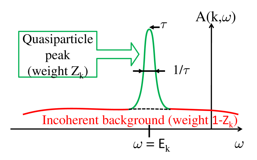
Figure 5: A cartoon of the spectral function for interacting particle. One can recognize several features. There is a continuous background of excitations of total weight $1-Z_{k}$. This part of the spectrum cannot be identified with excitations that resemble quasi-free particles. In addition to this continuous background there can be a quasiparticle peak. The total weight of the peak is $Z_{k}$ determined by the real part of the self energy. The center of the peak is at an energy $E(k)$ which is renormalized by the interactions compared to the independent electron dispersion $\xi(k)$. This change of dispersion defines an effective mass $m^{*}$ determined also by the real part of the self energy. The quasiparticle peak has a lorentzian lineshape that traduces the finite lifetime of the quasiparticles. The lifetime is inversely proportional to the imaginary part of the self energy.

Quite generally we can thus distinguish two parts in the spectral function. There is a continuous background, without any specific feature for which the probability to find a particle with an energy $\omega$ is practically independent of its momentum $k$. This part of the spectrum cannot be easily identified with excitations resembling free or quasi-free particles. On the other hand, in addition to this part, which carries a total spectral weight $1-Z_{k}$, another part of the excitations gives a spectral weight with a lorentzian peak, well centered around a certain energy $E(k)$. This part of the spectrum can thus be identified with a “particle”, called Landau quasiparticle, with a well defined relation between its momentum $k$ and energy $\omega=E(k)$. This quasiparticle has a only a finite lifetime, determined by the inverse width and height of the peak. The dispersion relation and the total weight of the quasiparticle peak are controlled by the real part of the self energy, while the lifetime is inversely proportional to the imaginary part. Depending on the self energy, and thus the interactions, we can still have objects that we could identify with “free” particles, solving our problem of why the free electron picture works qualitatively so well with just a renormalization of the parameters such as the mass into an effective mass.

However it is not clear that in the presence of interactions one can have sharp quasiparticles. In fact one would naively expect exactly the opposite. Indeed we would like to identify the peak in the spectral function with the existence of a quasiparticle. The energy of this excitation is $E(k)$ which of course tends towards zero at the Fermi level, while the imaginary part of the self energy is the inverse lifetime $1/\tau$. Since $E(k)$ gives the oscillations in time of the wavefunction of the particle $e^{-iE(k)t}$, in order to be able to identify properly a particle it is mandatory, as shown in Fig. 6

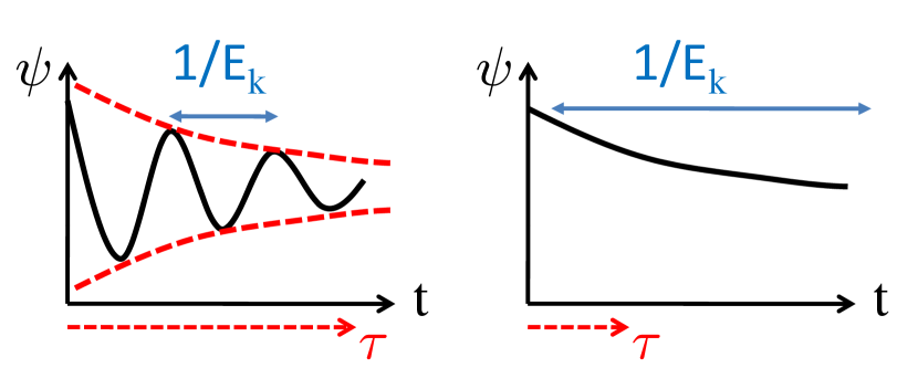
Figure 6: For particles with an energy $E(k)$ and a finite lifetime $\tau$, the energy controls the oscillations in time of the wavefunction. (left) In order to properly identify an excitation as a particle it is mandatory that the wavefunction can oscillate several time before being damped by the lifetime, otherwise it is impossible to precisely define the frequency of the oscillations. This is illustrated on the left part of the figure. (right) On the contrary if the damping is too fast, one cannot define an average energy and thus identify the excitation with a particle.

that there are many oscillations by the time the lifetime has damped the wavefunction. This imposes

$$E(k)^{-1}\gg\tau$$ (35)

Since $1/\tau$ is the imaginary part of the self energy and controlled by energy scales of the order of the interactions, one would naively expect the life time to be roughly constant close to the Fermi level. On the other hand one has always $E(k)\to 0$ when $k\to k_{\text{F}}$, and thus the relation (35) to be violated when one gets close to the Fermi level. This would mean that for weak interactions one has perhaps excitations that resemble particles far from the Fermi level, but that this becomes worse and worse as one looks at low energy properties, with finally all the excitations close to Fermi level being quite different from particles. Quite remarkably, as was first shown by Landau, this “intuitive” picture is totally incorrect and the lifetime has a quite different behavior when one approaches the Fermi level.

Quasiparticle scattering:

In order to estimate the lifetime let us look at what excitations can lead to the scattering of a particle from a state $k$ to another state. Let us start from the non interacting ground state in the spirit of a perturbative calculation in the interactions. As shown in Fig. 7

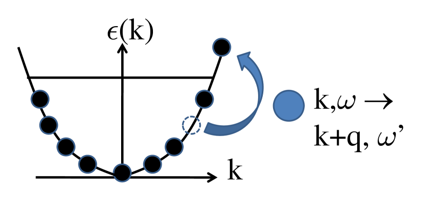
Figure 7: Cartoon of the process giving the lifetime of a particle with energy $\omega$. It can interact with the ground state of the system, which has all single particle states filled below the Fermi energy $E_{\text{F}}$. The excitations are thus particle hole excitations where a particle is promoted from below the Fermi level to above the Fermi level. Due to the presence of the sharp Fermi level, the phase space available for making such particle hole excitations is severely restricted.

a particle coming in the system with an energy $\omega$ and a momentum $k$ can excite a particle-hole excitation, taking a particle below the Fermi surface with an energy $\omega_{1}$ and putting it above the Fermi level with an energy $\omega_{2}$. The process is possible if the initial state is occupied and the final state is empty. One can estimate the probability of transition using the Fermi golden rule. The probability of the transition gives directly the inverse lifetime of the particle, and thus the imaginary part of the self energy. We will not care here about the matrix elements of the transition, assuming that all possible transitions will effectively happen with some matrix element. The probability of transition is thus the sum over all possible initial states and final states that respect the constraints (energy conservation and initial state occupied, final state empty). Since the external particle has an energy $\omega$ it can give at most $\omega$ in the transition. Thus $\omega_{2}-\omega_{1}\leq\omega$. This implies also directly that the initial state cannot go deeper below the Fermi level than $\omega$ otherwise the final state would also be below the Fermi level and the transition would be forbidden. The probability of transition is thus

$$P\propto\int_{-\omega}^{0}d\omega_{1}\int_{0}^{\omega+\omega_{1}}d\omega_{2}=\frac{1}{2}\omega^{2}$$ (36)

One has thus the remarkable result that because of the discontinuity due to the Fermi surface and the Pauli principle that only allows the transitions from below to above the Fermi surface, the inverse lifetime behaves as $\omega^{2}$. This has drastic consequences since it means that contrarily to the naive expectations, when one considers a quasiparticle at the energy $\omega$, the lifetime grows much faster than the period $D\sim 1/\omega$ characterizing the oscillations of the wavefunction. In fact

$$\frac{\tau}{D}=\frac{1}{\omega}\to\infty$$ (37)

when one approaches the Fermi level. In other words the Landau quasiparticles become better and better defined as one gets closer to the Fermi level. This is a remarkable result since it confirms that we can view the system as composed of single particle excitations that resemble the original electrons, but with renormalized parameters (effective mass $m^{*}$ and quasiparticle weight $Z_{k}$). Other quantum numbers are the same than the ones of an electron (charge, spin). Note that this does not mean that close to the Fermi level the interactions are disappearing from the system. They are present and can be extremely strong, and affect both the effective mass and quasiparticle weight very strongly. It is only the scattering of the quasiparticles that is going to zero when one is going close to the Fermi level. This is thus a very unusual situation quite different from what would happen in a classical gas. In such a case diluting the gas would thus reduce both the interaction between the particles and also their scattering in essentially the same proportion. On the contrary in a Fermi liquid there are many $\mathcal{N}\to\infty$ electrons in the ground state, which are in principle strongly affected by the interactions. Note again that computing the ground state would be a very complicated task. However there are very few excitations above this ground state at low energy. These excitations can interact strongly with the other electrons in the soup of the ground state, leading to a very strong change of the characteristics compared to free electron excitations. This can lead to very large effective masses or small quasiparticle weight. On the other hand the lifetime of the quasiparticles is controlled by a totally different mechanism since it is blocked by the Pauli principle, as shown in Fig. 3. Thus even if the interaction is strong the phase space available for such a scattering is going to zero close to the Fermi level, making the quasiparticle in practice infinitely long lived particles, and allowing to use them to describe the system. The image of Fig. 7 also gives us a description of what a quasiparticle is: this is an electron that is surrounded by a cloud of particle-hole excitations, or in other words density fluctuations since $c^{\dagger}_{k+q}c_{k}$ is typically the type of terms entering the density operator. Such density fluctuations are of course neutral and do not change the spin. This composite object electron+density fluctuation cloud, thus represent a tightly bound object (just like an electron does dress with a cloud of photons in quantum electrodynamics), that is the Landau quasiparticle. Since the electron when moving must carry with it its polarization cloud, one can guess that its effective mass will indeed be affected.

The Fermi liquid theory is a direct explanation of the fact that “free” electrons theory works very well qualitatively (such as the specific heat linear in temperature) even when the change of parameters can be huge. We show in Fig. 8 the case of systems where the renormalization of the mass is about $m^{*}\sim 10^{3}m$ indicating very strong interactions effects.

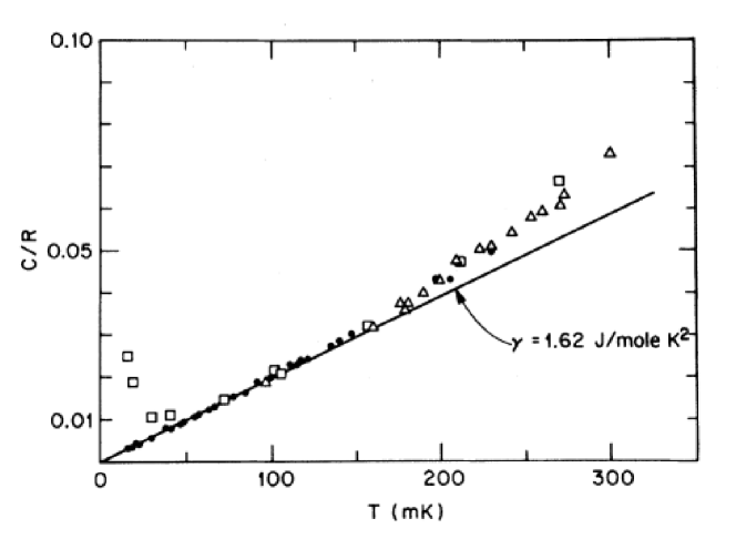
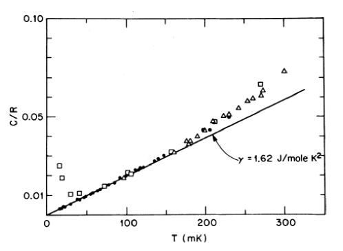
Figure 8: Physical properties of the compound CeAl₃. (top) The specific heat is linear in temperature $T$, but the slope gives an effective mass of about $10^{3}$m showing extremely strong interaction effects, showing that the Fermi liquid theory applies even when the interaction effects are strong. (bot) The resistivity varies as $T^{2}$ in very good agreement with the Fermi liquid theory. [After [Andres et al. (1975)]]

Nevertheless we see that the specific heat varies linearly with temperature just like for free electrons. The prediction for the quasiparticle peaks fits very well with the photoemission data of Fig. 2, in which one clearly sees the peaks becoming sharper as one approaches the Fermi level. There is another direct consequence of the prediction for the lifetime. At finite temperature one can expect the lifetime to vary as $\tau\sim 1/T^{2}$ since $T$ is the relevant energy scale when $T\gg\omega$. If we put such a lifetime in the Drude formula for the conductivity we get

$$\sigma(T)=\frac{ne^{2}\tau}{m}\propto\frac{1}{T^{2}}$$ (38)

This result can be confirmed by a full calculation. This shows that the electron-electron interactions give an intrinsic contribution to the resistivity that varies as $\rho(T)\sim T^{2}$, and which also can be taken as one of the characteristic of Fermi liquid behavior. This is however difficult to test since this temperature dependence can easily be masked by other scattering phenomena (impurities, scattering by the phonons etc.) that must be added to the electron-electron scattering and that have quite different temperature dependence. Nevertheless there are some materials where the $T^{2}$ law can be well observed as shown in Fig. 8. Another interesting consequence can be deduced by looking at the occupation factor $n(k)$ which can be expressed from the spectral function by

$$n(k)=\int d\omega^{\prime}A(k,\omega^{\prime})f_{\text{F}}(\omega^{\prime})$$ (39)

For free electrons one recovers the step function at $k=k_{\text{F}}$. For a Fermi liquid, if we represent the spectral function as

$$A(k,\omega)=Z_{k}\delta(\omega-E(k))+A_{{\rm inc}}(k,\omega)$$ (40)

where the incoherent part is a smooth flattish function without any salient feature, then $n(k)$ becomes

$$n(k)=Z_{k}f_{\text{F}}(E(k))+Cste$$ (41)

Thus even in the presence of interaction there is still a discontinuity at the Fermi level, that is only rounded by the temperature. Contrarily to the case of free electron the amplitude of the singularity at $T=0$ is not one anymore but is now $Z_{k_{\text{F}}}<1$. The existence of this discontinuity if quasiparticle exists tells us directly that the Fermi liquid theory is internally consistent since the very existence of the quasi particles (namely the large lifetime) was heavily resting on the existence of such a discontinuity at the Fermi level. One can thus in a way consider that the existence of a sharp discontinuity at the Fermi level is a good order parameters to characterize the existence of a Fermi liquid.

One important question is when the Fermi liquid theory does apply. This is of course a very delicate issue. One can see both from the arguments given above, and from direct perturbative calculations that when the interactions are weak the Fermi liquid theory will in general be valid. There are some notable exceptions that we will examine in the next section, and for which the phase space argument given above fails. However the main interest of the Fermi liquid theory is that it does not rest on the fact that the interactions are small and, as we have seen through examples, works also remarkably well for the case of strong interactions, even when all perturbation theory fails to be controlled. This is specially important for realistic systems since, as we showed, the interaction is routinely of the same order than the kinetic energy even in very good metals. The Fermi liquid theory has thus been the cornerstone of our description of most condensed matter systems in the last 50 years or so. Indeed it tells us that we can “forget” (or easily treat) the main perturbation, namely the interaction among fermions, by simply writing what is essentially a free fermion Hamiltonian with some parameters changed. It is not even important to compute microscopically these parameters since one can simply extract them from one experiment and then use them consistently in the others. This allows to go much further and treat effects caused by much smaller perturbations that one would otherwise have been totally unable to take into account. One of the most spectacular examples is the possibility to now look at the very tiny (compared to the electron-electron interactions) electron-phonon coupling, and to obtain from that the solution to the phenomenon of superconductivity, or other instabilities such as magnetic ordering.

3 Beyond Fermi liquid

Of course not all materials follow the Fermi liquid theory. There are cases when this theory fails to apply. In that case the system is commonly referred to as strongly correlated or “non Fermi liquid” a term that hides our poor knowledge of their properties. For such systems, the question of the effects of interactions becomes again a formidable problem. As discussed in the introduction, most of the actual research in now devoted to such non fermi liquid systems.

There are fortunately some situation where one can understand the physics and we will examine such cases in this section as well as define the main models that are at the heart of the study of these systems.

1 Instabilities of the FL

The Fermi liquid can become unstable for a variety of reasons. Some of them are well known.

The simplest instability consists, at low temperature, for the system to go an ordered state. Many type of orders are possible, the most common are spin order such as ferromagnetism, antiferromagnetism, charge order such as a charge density wave, or superconductivity. In general analyzing such instabilities can be done by computing the corresponding susceptibility and looking for divergences as the temperature is lowered. When the normal system is well described by a Fermi liquid it is in general relatively easy to compute these susceptibilities by a mean field decoupling of the interaction. This is of course much more complex when one starts from a normal phase which is a non Fermi liquid.

Another important ingredient in the stability of the Fermi liquid phase is the dimensionality of the system. Intuitively we can expect that the lower the dimension the more important the effects of the interactions will be since the particles have a harder time to avoid each other. The ultimate case in that respect is the one dimensional situation where one particle moving will push the particle in front and so on, as anybody queuing in a line had already has chance to notice. This effect of dimensionality is confirmed by a direct perturbative calculation of the self energy [Mahan (1981), Abrikosov et al. (1963)]

$$\begin{split}\Sigma_{3D}(\omega)&\propto U^{2}\omega^{2}\\ \Sigma_{2D}(\omega)&\propto U^{2}\omega^{2}\log(\omega)\\ \Sigma_{1D}(\omega)&\propto U^{2}\omega\log(\omega)\end{split}$$ (42)

where $U$ is the strength of the interaction. In particular one immediately see that for the one dimensional case, the self energy becomes dominant compared to the mean energy $\omega$. Using (33) one sees that for one dimension the quasiparticle weight is zero at the Fermi level. This means the whole argument we used in the previous section to justify the existence of sharper and sharper peaks an thus the existence of Landau quasiparticles fails regardless of the strength of the interaction. In one dimension Fermi liquid always fails. This leads to a remarkable physics that we examine in more details in Section 4.

With the exception of the one dimensional case, one can thus expect the Fermi liquid to be perturbatively valid in two dimensions and above. Of course if the interaction becomes large whether a non Fermi liquid state can appear is one of the major challenges of today’s research.

2 Tight binding and Hubbard Hamiltonian

One ingredient of special important is the presence of a lattice on which the fermions can move. This is the normal situation in solids, with the presence of the ionic lattice, and can be realized very well in cold atomic systems by imposing an optical lattice. Even for free electrons the lattice is an essential ingredient, since it leads to the existence of bands of energy.

One very simple description of the effects of a lattice is provided by the tight binding model [Ziman (1972)]. This model is of course an approximation of the real band structure in solids, but contains the important ingredients. Recently cold atomic systems in optical lattices have provided excellent realization of such a model, and we recall here its main features.

Let us consider of cold atoms of fermions or bosons [Anglin and Ketterle (2002)]. Such system can be described by

$$H=\int dr\frac{\hbar^{2}(\nabla\psi)^{\dagger}(\nabla\psi)}{2m}+\frac{1}{2}\int dr\;dr^{\prime}\;V(r-r^{\prime})\rho(r)\rho(r^{\prime})-\int dr\;\mu(r)\rho(r)$$ (43)

The first term is the kinetic energy, the second term is the interaction $V$ between the particles and the last term is the chemical potential. The three dimensional interaction is characterized by a scattering length [Pitaevskii and Stringari (2003)] $a_{s}$

$$V(x,y,z)=V_{0}\delta(x)\delta(y)\delta(z)=\frac{4\pi\hbar^{2}a_{s}}{m}\delta(x)\delta(y)\delta(z)$$ (44)

The chemical potential takes into account the confining potential $V_{c}(r)$ keeping the particles in the trap

$$\mu(\vec{r})=\mu_{0}-V_{c}(r)=\mu_{0}-\frac{1}{2}\omega_{0}r^{2}$$ (45)

and is thus in general position dependent. In presence of interactions the effect of the confining potential can usually be taken by making a local density approximation. If one neglects the kinetic energy (so called Thomas-Fermi approximation; for other situations see [Pitaevskii and Stringari (2003)]) the density profile is obtained by minimizing (43) and (45), leading to

$$V_{0}\rho(r)+[V_{c}(r)-\mu_{0}]=0$$ (46)

the density profile is thus an inverted parabola, reflecting the change of the chemical potential. In the following we will ignore for simplicity the confining potential and consider the system as homogeneous.

If one adds an optical lattice, produced by counter propagating lasers, to the system it produces a periodic potential of the form $V_{L}(x)$ coupled to the density [Bloch et al. (2008)]

$$H_{L}=\int dx\;V_{L}(x)\rho(x)$$ (47)

This term, which favors certain points in space for the position of the bosons, mimics the presence of a lattice of period $a$, the periodicity of the potential $V_{L}(x)$. We take the potential as

$$V_{L}(x)=V_{L}\sum_{\alpha=1}^{d}\sin^{2}(k_{a}r_{\alpha})=\frac{V_{L}}{2}\sum_{\alpha=1}^{d}[1-\cos(2k_{\alpha}r_{\alpha})]$$ (48)

one has thus $a=\pi/k_{\alpha}$ as the lattice spacing.

If the lattice amplitude $V_{L}$ is large then it is possible to considerably simplify the full Hamiltonian. In that case on can focuss on the solution in one of the wells of the optical lattice, as shown in Fig. 9.

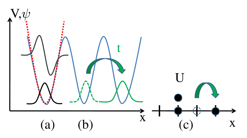
Figure 9: Optical lattices and tight binding model. (a) If the optical lattice is deep enough one can consider the wells as practically independent and obtain the states in each well. Since the well can be approximated by a parabolic potential one has harmonic oscillator states. (b) Some level of overlap exists between the wavefunctions of different wells. This provide a hopping amplitude $t$ for a particle to move from one well to the next. Similarly the interaction between particles is only efficient if the two particles are in the same well. (c) The system can be mapped on a tight binding model, describing particles leaving on the sites of a lattice and hopping from one site to the next with an amplitude $t$. If interactions are included they can be modelled by local interactions of strength $U$. The resulting Hamiltonian is the famous Hubbard model.

The well can be approximated by a parabola $\frac{1}{2}(4V_{L})k^{2}r^{2}$ and the solutions are those of an harmonic oscillator. The ground state one is

$$\psi_{0}(x)=\left(\frac{m\omega_{0}}{\hbar\pi}\right)^{1/4}e^{-\frac{m\omega_{0}}{2\hbar}x^{2}}$$ (49)

and higher excited states are schematically indicated on Fig. 9. Typical values for the above parameters are $a_{s}\sim 5nm$ while $a\sim 400nm$ [Stöferle et al. (2004)].

If $V_{L}$ is large the energy levels in each well are well separated and one can retain only the ground state wavefunction in each well, higher excited state being well separated in energy. On can thus full represent the state of the system by a creation (or destruction) of a particle in the $i$-th well (i.e. with the wavefunction (49)). One has thus the energy

$$H=E_{0}\sum_{u}c^{\dagger}_{i}c_{i}$$ (50)

This is just a chemical potential term and can be absorbed in the chemical potential. Of course if the lattice is not infinite, as indicated on Fig. 9 the wavefunction in different wells overlap, and there is an hybridation term $t$ between the wavefunction in two adjacent wells. This term allows the particle to go from one well to the next. For an optical lattice one gets [Zwerger (2003)]

$$t/E_{r}=(4/\sqrt{\pi})(V_{L}/E_{r})^{(3/4)}\exp{(-2\sqrt{V_{L}/E_{r}})}$$ (51)

Here $E_{r}=\hbar^{2}k^{2}/(2m)$ is the so called recoil energy, i.e. the kinetic energy for a momentum of order $\pi/a$. In presence of such term the energy becomes (we have written it for two spin species)

$$H_{t}=-t\sum_{\langle ij\rangle,\sigma}c^{\dagger}_{i\sigma}c_{j\sigma}-\sum_{i}\mu_{i\sigma}c^{\dagger}_{i\sigma}c_{i\sigma}$$ (52)

where $\langle\rangle$ denotes nearest neighbors. In Fourier space one recovers (1) with

$$\xi(\vec{k})=-2t\sum_{j=1}^{d}\cos(k_{j}a)$$ (53)

where $d$ is the dimension of space, $a$ the lattice spacing (I assumed here for simplicity a square lattice). The momentum $\vec{k}$ is restricted to the First Brillouin zone

$$k_{j}\in[-\pi/a,\pi/a]$$ (54)

Thus one particle per site corresponds to an half filled zone (half of the available states are occupied). For example in one dimension this gives $k_{\text{F}}=\pi/(2a)$. For independent fermions this is the best situation to have a metallic state since the Fermi level is far from a band edge. An empty band and a completely filled band (two particles per site) correspond to an insulating state. For a filled band all the excitations are blocked by the Pauli principle. The tight binding description of the kinetic energy contains thus the essential ingredient of quantum periodic systems namely the existence of bands, and the existence of a Brillouin zone.

One can add to this description, the effects of interaction. In a solid, as we discussed, the interaction is screened. A good approximation is thus to take a local interaction. For optical lattice such an approximation is truly excellent. Indeed, since atoms are neutral the interaction (44) has a range much smaller than the size of the well. Thus atoms only interact if they are in the same well of the optical lattice. One can thus represent the interaction by a purely local term

$$H_{U}=U\sum_{i}n_{i\uparrow}n_{i\downarrow}$$ (55)

The effective potential $U$ can be easily computed by using the shape of the on site wave function (49) with $\omega_{0}^{2}=4V_{L}k^{2}$

$$U=\int dxdydz|\psi(x,y,z)|^{4}$$ (56)

where $\psi(x,y,z)=\psi_{0}(x)\psi_{0}(y)\psi_{0}(z)$.

The full Hamiltonian of the system is thus

$$H=H_{t}+H_{U}$$ (57)

and describes particle hopping on a lattice with a purely local repulsion. This is the famous Hubbard model. This model, although extremely simple contains the essential ingredients of interacting fermions. Optical lattices are thus excellent realizations of this model. They offer in addition a powerful control on the ratio of $U/t$ the interaction measured compared to the kinetic energy, since we see that by increasing the height of the optical lattice one essentially modifies the overlap integral $t$ between two different sites [Jaksch et al. (1998), Greiner et al. (2002)]. Recently cold atomic systems have also provided a direct control over the interaction $U$ by using a Feshbach resonance [Bloch et al. (2008)].

3 Mott insulators

Let us now study the properties of interacting fermions on a lattice as described in the previous section. For noninteracting fermions, the system remains metallic unless the band is completely filled. The situation changes drastically in presence of interactions. The combination of lattice and interactions leads to a striking effect of interactions known as the Mott transition, a phenomenon predicted [Mott (1949)] by Sir Nevil Mott (see Fig. 10)

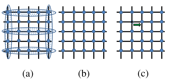
Figure 10: (top) Sir Nevil Mott. (a) If the repulsion is weak the particles prefer to gain kinetic energy and are essentially in delocalized (plane wave) state. This leads to a metallic state, and usually to a Fermi liquid. (b) For one particle per site $n=1$ and strong interactions the system prefers to localize the particles, not to pay the large repulsion energy. This leads to a Mott insulating site. Residual kinetic energy tends to favor antiferromagnetic exchange between nearest neighbors, to avoid Pauli principle blocking. Depending on the lattice this can lead to various type of magnetic order. (c) If there are less than one particle per site $n<1$ but the interaction is large, a state with only one particle per site is still favored. The conduction is only providing from the holes present in the system that can hop at no interaction cost. Although this is still a metallic state this state has quite different properties than the weakly correlated one described in (a).

To understand the phenomenon, let us consider a simple variational calculation of the energy of the Hubbard model (57), assuming that the system is described by a FL like ground state. We will be even more primitive and take free electrons. In that case the ground state is simply the Fermi sea (2). The energy of such a state $E_{0}=\langle\psi_{0}|H\left|\psi_{0}\right\rangle$ is simply given by

$$E_{0}=2\sum_{|k|<k_{\text{F}}}\epsilon(k)+U\sum_{i}\langle\psi_{0}|n_{i\uparrow}n_{i\downarrow}\left|\psi_{0}\right\rangle$$ (58)

where the dispersion relation is (53). The first term in (58) is simply the average of the kinetic energy

$$\int_{-W}^{\mu_{0}}d\epsilon\mathcal{N}(\epsilon)\epsilon=\Omega\int_{-W}^{\mu_{0}}d\epsilon n(\epsilon)\epsilon=\Omega\epsilon_{0}$$ (59)

where $\Omega$ is the number of sites in the systems, $n(\epsilon)$ the density of states per site, $W$ the minimum of energy in the band and $\mu_{0}$ the chemical potential. For the dispersion relation (53), $\epsilon_{0}$ is a filling dependent negative number (for $n\leq 1$). The second term in (58) depends on the average number of doubly occupied sites. Because the plane waves of the ground state have a uniform amplitude on each site

$$\langle n_{i\uparrow}n_{i\downarrow}\rangle=\langle n_{i\uparrow}\rangle\langle n_{i\downarrow}\rangle=\frac{n^{2}}{4}$$ (60)

and thus

$$E_{0}=\Omega[\epsilon_{0}+U\frac{n^{2}}{4}]$$ (61)

One can notice two interesting points on this equation: i) in the absence of interaction ($U=0$) the system gains energy by delocalizing the particles. The maximum gain in energy, so in a way the best metallic state, is obtained when the band is half filled $n=1$; ii) if the system has a FL (free electron like) ground state, the energy cost due to the interactions is growing. Thus one could naively expect that for large $U$ a better state could occur. Let us consider for example a variational function in which each particle is localized on a given site (for simplicity let us only consider $n\leq 1$)

$$\left|\psi_{M}\right\rangle=c^{\dagger}_{i_{1},\uparrow}\cdots c^{\dagger}_{i_{N},\downarrow}\left|\varnothing\right\rangle$$ (62)

Note that we can put the spins in an arbitrary order for the moment. There are thus many such states $\left|\psi_{M}\right\rangle$ differing by their spin orientation. What is the best spin order will be discussed in the next section. One has obviously

$$\langle\psi_{M}|H\left|\psi_{M}\right\rangle=0$$ (63)

since there is no kinetic energy and no repulsion given the fact that at most one particle is on a given site. We can now take these two states as variational estimates of what could be the best representation of the ground state of our system, the idea being that the wavefunction with the lower energy is the one that has probably the largest overlap with the true ground state of the system. At a pure variational level, this calculation would strongly suggest that the wave function $\left|\psi_{0}\right\rangle$ is a good approximation of the ground state at small interaction while $\left|\psi_{M}\right\rangle$ would be the best approximation of the ground state at large $U$. One could thus naively expect a crossover or even a quantum phase transition at a critical value of $U$. The nature of the two “phases” can be inferred from the two variational wavefunction. For small $U$ one expects a good FL, while for large interactions one can expect a state where the particles are localized. For $n=1$, as shown in Fig. 10, such a state would be an insulator. One could thus expect a metal insulator transition, driven by the interactions at a critical value of the interactions $U$ of the order of the kinetic energy per site $\epsilon_{0}$ of the non interacting system. Of course our little variational argument is far too primitive to allow to seriously conclude on the above points, and one must perform more sophisticated calculations [Imada et al. (1998)]. This includes physical arguments, more refined variational calculations [Gutzwiller (1965), Brinkman and Rice (1970), Yokoyama and Shiba (1987)], slave bosons techniques [Kotliar and Ruckenstein (1986)] and refined mean field theories [Kotliar and Vollhardt (2004)].

As it turns out our little calculation gives already the right physics, originally understood by Mott. An important ingredient is the filling of the band. Indeed the situation is extremely different depending on whether the filling is one particle per site or not. If the filling is one particle per site (half filled band), then our little variational state, with one particle per site is indeed an insulator as shown on Fig. 10. Applying the kinetic energy operator on this state would force it to go through a state with at least a doubly occupied site, with an energy cost of $U$, so such excitations could not propagate. Such an insulating state created by interactions has been nicknamed a Mott insulator. From the point of view of band theory and free electrons this is a remarkable state, since a half filled system would give normally the best type of metallic state possible. We see that interactions are able to transform this state into an insulating state.

If the filling is not exactly one particle per site, something remarkable occurs again when $U>U_{c}$. In that case, as shown in Fig. 10, the function were one has only singly occupied sites is obviously still a very good starting point. However if there are now empty sites ($n<1$) these holes can now propagate freely at no cost in $U$. Such a state is thus not an insulator but still a metal. There are important differences with the metal one would get for small $U$. Indeed in this strongly correlated metal, only the holes can propagate freely, and one can expect that the number of carriers will be proportional to the doping $n-1$ and not to the total number of particles $n$ in the system. Other properties are also affected. I will not address in details these points but refer the reader to the literature for more details.

To finish let me mention three important points: the first one is that some additional phenomena can shift the Mott transition to $U=0$ for special lattices. Indeed if the lattice is bipartite, i.e. can be separated in two sublattices which are connected only be the hopping operator, special properties occur. This is in particular the case of the square or the hexagonal lattice. On such lattices, for one particle per site the dispersion relation has a special property known as nesting property. Namely there is a wavevector $Q$ such that for all $k$

$$\xi(k+Q)=-\xi(k)$$ (64)

For the tight-binding relation on a square lattice, nesting occurs for $n=1$ and $Q=(\pi,\pi,\cdots)$. When a Fermi surface is nested the charge and spin susceptibilities have a logarithmic divergence due to the nesting. Typically

$$\chi(Q,T)\simeq\mathcal{N}(E_{\text{F}})\log[\beta W]$$ (65)

This divergent susceptibility provokes an instability of the metallic state for arbitrary interactions. As a result, nested systems become Mott insulators as soon as the interactions become repulsive, and order antiferromagnetically (at least in $d=3$ where quantum fluctuations cannot destroy the magnetic order).

The second remark is that Mott insulators are not limited to the case of one particle per site. Any commensurate filling can potentially lead to an insulating state, depending on the range of the interactions. For example one can expect an insulating state at $1/4$ filling if both on site and nearest neighbor interactions are present and of sufficient strength.

The third important point is that nothing in such a mechanism limits Mott insulators to fermionic statistics. As we saw in the simple derivation, interactions are simply avoiding double occupancy, which turns the system into an insulator. So we can also expect Mott insulators to exist for bosons and even for Bose-Fermi mixtures. The Mott phase will be essentially the same in each case (only one particle per site), but of course the low interaction phase will strongly depend on the precise properties of the system (e.g. for bosons one can expect to have a superfluid phase at small interactions).

Mott insulators are one of the most spectacular effects of strong correlations. They are ubiquitous in nature and occur in oxides, cuprates, organic conductors and of course are realized in cold atomic systems both for bosons and fermions.

4 Magnetic properties of Mott insulators

Let me concentrate now on the Mott phase ($n=1$) at large interactions $U>U_{c}$. In that case, at low temperature all charge excitations are gapped, with a gap $\Delta\sim U$ and the system is an insulator. One could thus naively think that one has properties very similar to the ones of a band insulator. Although this naive expectation is, to some extent correct for the charge properties, it is completely incorrect for the spin ones, and very interesting spin physics occurs. Indeed a band insulators corresponds to either zero or two particles per site. It means that in both case the on site spin is zero. The Pauli principle forces two particles on the same site to be in a singlet spin state to get a fully antisymmetric wave function. Thus a band insulator has no interesting charge nor spin properties. This is not the case for Mott insulator since each site is singly occupied. There is thus a spin $1/2$ degree of freedom on each site, and it is thus important to understand the corresponding magnetic properties. This was worked out [Anderson (1959)] by P. W. Anderson (see Fig. 11).

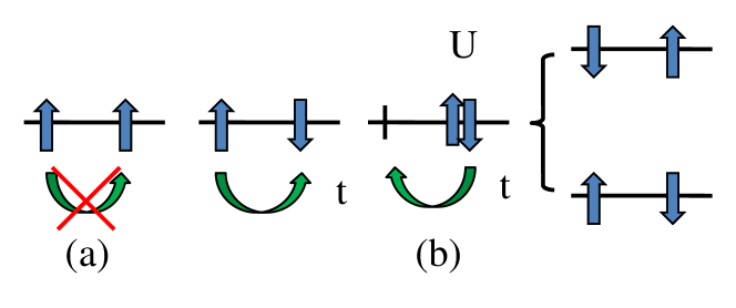
Figure 11: (top) P. W. Anderson. (a) The hopping between two neighboring identical spins is totally blocked by the Pauli principle. The system cannot gain some residual kinetic energy in this case. (b) If the spins are antiparallel then the kinetic energy can allow virtual hopping through an intermediate state of energy $U$. This state comes back either to the original state or to a configuration in which the spins have been exchanged. This is the mechanism of superexchange leading to dominant antiferromagnetic correlations for fermionic Mott insulators.

To do so let us examine the case of two sites. The total Hilbert space is

$$\left|\uparrow,\downarrow\right\rangle,\left|\downarrow,\uparrow\right\rangle,\left|\uparrow\downarrow,0\right\rangle,\left|0,\uparrow\downarrow\right\rangle,\left|\uparrow,\uparrow\right\rangle,\left|\downarrow,\downarrow\right\rangle$$ (66)

Since the states are composed of Fermions one should be careful with the order of operators to avoid minus signs. Let us take the convention that

$$\begin{split}\left|\uparrow,\downarrow\right\rangle=c^{\dagger}_{1\uparrow}c^{\dagger}_{2\downarrow}\left|\varnothing\right\rangle\quad&,\quad\left|\downarrow\uparrow\right\rangle=c^{\dagger}_{1\downarrow}c^{\dagger}_{2\uparrow}\left|\varnothing\right\rangle\\ \left|\uparrow\downarrow,0\right\rangle=c^{\dagger}_{1\uparrow}c^{\dagger}_{1\downarrow}\left|\varnothing\right\rangle\quad&,\quad\left|0,\uparrow\downarrow\right\rangle=c^{\dagger}_{2\uparrow}c^{\dagger}_{2\downarrow}\left|\varnothing\right\rangle\end{split}$$ (67)

The states with two particles per site are states of energy $\sim U$ and therefore strongly suppressed. We thus need to find what is the form of the Hamiltonian when restricted to the states with only one particle per site. It is easy to check that the two states $\left|\uparrow\uparrow\right\rangle$ and $\left|\downarrow\downarrow\right\rangle$ are eigenstates of $H$

$$H\left|\uparrow\uparrow\right\rangle=0$$ (68)

and a similar equation for $\left|\downarrow\downarrow\right\rangle$. The reason why the kinetic energy does not act on such a state is shown in Fig. 11. The Pauli principle block the hopping if the two spins are equal. On the contrary, if the two spins are opposite the particles can make a virtual jump on the neighboring site. Since this state is of high energy $U$ the particles must come back to the original position, or the two particles can exchange leading to a term similar to a spin exchange (see Fig. 11). The kinetic energy thus leads to a magnetic exchange, named superexchange, that will clearly favor configurations with opposite neighboring spins, namely will be antiferromagnetic.

Let us now quantify the mechanism. The Hamiltonian can be written in the basis (66) (only the action on the first four states is shown since $\left|\uparrow\uparrow\right\rangle$ and $\left|\downarrow\downarrow\right\rangle$ are eigenstates and thus are uncoupled to the other ones)

$$H=\left(\begin{array}[]{cccc}0&0&-t&-t\\ 0&0&t&t\\ -t&t&U&0\\ -t&t&0&U\end{array}\right)$$ (69)

This Hamiltonian couples the low energy states with one particle per site to high energy states of energy $U$. In order to find the restriction of $H$ to the low energy sector, let us first make a canonical transformation of $H$

$$H^{\prime}=e^{iS}He^{-iS}\simeq H+i[S,H]+\frac{i^{2}}{2}[S,[S,H]]+\cdots$$ (70)

where the matrix $S$ is expected to be perturbative in $t/U$. In this transformation one wants to chose the matrix $S$ such that

$$H_{t}+i[S,H_{U}]=0$$ (71)

This will ensure that $H^{\prime}$ has no elements connecting the low energy sector with the sector of energy $U$. The restriction of $H^{\prime}$ to the low energy sector will thus be the Hamiltonian we need to diagonalize to find the spin properties.

Using the condition (71) and keeping only terms up to order $t^{2}/U$ it is easy to check that

$$H^{\prime}=H_{U}+\frac{i}{2}[S,H_{t}]$$ (72)

Since $H$ is block diagonal one can easily determine $S$ to be

$$S=\frac{i}{U}\left(\begin{array}[]{cccc}0&0&-t&-t\\ 0&0&t&t\\ t&-t&0&0\\ t&-t&0&0\end{array}\right)$$ (73)

This leads using (72) to

$$H^{\prime}=\frac{4t^{2}}{U}[\frac{1}{2}[\left|\uparrow\downarrow\right\rangle\langle\downarrow\uparrow|+\left|\downarrow\uparrow\right\rangle\langle\uparrow\downarrow|]-\frac{1}{2}[\left|\uparrow\downarrow\right\rangle\langle\uparrow\downarrow|+\left|\downarrow\uparrow\right\rangle\langle\downarrow\uparrow|]$$ (74)

This Hamiltonian must be complemented by the fact that $H^{\prime}\left|\uparrow\uparrow\right\rangle=0$. Since there is one particle per site, it can now be represented by a spin $1/2$ operator $S^{\alpha}=\frac{1}{2}\sigma^{\alpha}$, where $\alpha=x,y,z$ and the $\sigma$ are the Pauli matrices. Using $S^{+}=S^{x}+iS^{y}$ for the raising spin operator one obtains

$$H^{\prime}=\frac{4t^{2}}{U}[\frac{1}{2}[S^{+}_{1}S^{-}_{2}+S^{-}_{1}S^{+}_{2}]+S^{z}_{1}S^{z}_{2}-\frac{1}{4}]$$ (75)

Up to a constant which is a simple shift of the origin of energies, the final Hamiltonian is thus the Heisenberg Hamiltonian

$$H=J\sum_{\langle ij\rangle}\vec{S}_{i}\cdot\vec{S}_{j}$$ (76)

where the magnetic exchange is $J=4t^{2}/U$.

As we saw for fermions, the exchange $J$ is positive and thus the system has dominant antiferromagnetic correlations. This explain naturally the remarkable fact that antiferromagnetism is quite common in solid state physics. Of course the magnetic properties depend on the lattice, and the Hamiltonian (76) can potentially lead to very rich physics [Auerbach (1998)]. It is important to note that we are dealing here with quantum spins for which $[S_{x},S_{y}]=iS_{z}$ and thus the three component of the spins cannot be determined simultaneously. Quantum fluctuation will thus drastically affect the possible spin orders. Depending on the lattice various ground states are possible ranging from spin liquids to ordered states.

5 Summary of the basic models

Let me summarize in this section the basic models that are commonly used to tackle the properties of strongly correlated systems. Of course these are just the simplest possible case, and many extensions and interesting generalization have been proposed. There is currently a great interest in realizing these models with cold atomic gases.

Fermions

The simplest interacting model on a lattice is the Hubbard model

$$H=-t\sum_{\langle ij\rangle,\sigma}c^{\dagger}_{i\sigma}c_{i\sigma}+U\sum_{i}n_{i\uparrow}n_{i\downarrow}$$ (77)

where $\langle\rangle$ denote the nearest neighbors, which of course depends on the topology of the lattice (square, triangular, etc.). Having only on site interactions this model can only stabilize a Mott insulating phase at half filling ($n=1$). If the lattice is bipartite (e.g. square), the Mott phase is stable for any $U>0$ and the ground state is an antiferromagnetic state. If the lattice is not bipartite, then a critical value of $U$ is normally requested to reach the Mott insulating state. The spin order then depends on the lattice (see the spin section below).

For $U<0$ this model has a BCS type instability leading to a superconducting ground state. There are interesting symmetries for the Hubbard model. In particular for bipartite lattices there is a particle-hole symmetry for one spin species that can map the repulsive Hubbard model onto the attractive one, and exchange the magnetic field and the chemical potential. This symmetry can be exploited in several context, but in particular can be very useful in the cold atom context for probing the phases of the repulsive Hubbard model in a much more convenient way [Ho et al. (2009)].

The canonical Hubbard model can be easily extended in several ways. Longer range hopping can be added, and of course longer range interactions than on-site can also be included. In that case insulating phases can in general be stabilized at other commensurate fillings. Finally one can also increase the number of states per site (so called multi-orbital Hubbard model), a situation that has been useful in condensed matter and also is potentially relevant for cold atoms in optical lattices, for example if one needs to take into account the higher states in each well of Fig. 9.

Bosons

Here also the canonical model is the Hubbard model (nicknamed Bose-Hubbard model in that case). The main difference is that the simplest case do not need spins for the bosons. The simplest Bose-Hubbard model is thus

$$H_{B}=-t\sum_{\langle ij\rangle}[b^{\dagger}_{i}b_{j}+b^{\dagger}_{j}b_{i}]+U\sum_{i}n_{i}(n_{i}-1)$$ (78)

This model has also in general a Mott transition for sufficiently large interaction when the filling is commensurate $n=1$ (1 boson per site) [Haldane (1981a), Fisher et al. (1989)]. In a similar way than for the fermions the model can be extended to the case of longer range hopping or longer range interactions, allowing for more insulating phases at other commensurabilities than for $n=1$.

The case of the Hubbard model with a nearest neighbor interaction

$$U\sum_{i}n_{i}(n_{i}-1)+V\sum_{\langle ij\rangle}n_{i}n_{j}$$ (79)

has an interesting property that is worth noting. When $U$ and $V$ are of the same order of magnitude, the system can have fluctuations of charge on a site going between zero, one and two bosons per site, since putting two bosons per site is a way to escape paying the repulsion $V$. The system is thus very close to a system with three state per site, i.e. of a system that can be mapped onto a spin $1$. In one dimension spin $1$ are known to have very special properties, and thus similar properties are expected for such an extended Hubbard model [Berg et al. (2009)]. In particular they can have a topologically ordered phase (Haldane phase [Haldane (1983)] for spin one). In higher dimensions such models can have complex orders, and there is in particular a debate on whether such models can sustain simultaneously a crystalline order (Mott phase for the bosons) and superfluidity, the so called supersolid phase [Niyaz et al. (1994), Wessel and Troyer (2005)].

Various extensions of the canonical Bose-Hubbard are worth noting. The most natural one, in connection with cold atomic systems is to consider a model with more than one species, in other word re-introducing a kind of “spin for the bosons”. This will correspond to bosonic mixtures. In that case one can generally expect interactions of the form

$$H=U_{\uparrow\uparrow}n_{\uparrow}(n_{\uparrow}-1)+U_{\downarrow\downarrow}n_{\downarrow}(n_{\downarrow}-1)+U_{\uparrow\downarrow}n_{\uparrow}n_{\downarrow}$$ (80)

Note that the $U_{\sigma\sigma}$ interactions did not exist for the fermionic Hubbard model because of the Pauli principle. For bosons their presence allow for a very rich physics. In particular the nature of the superexchange interactions will depend on the difference [Duan et al. (2003)] between the inter and the intra species interactions. If $U_{\uparrow\uparrow},U_{\downarrow\downarrow}\gg U_{\uparrow\downarrow}$ one is in a situation very similar to the case of fermions, with a dominant antiferromagnetic exchange. The ground state of such a model will be antiferromagnetic. On the contrary, if one is in the opposite situation then it is more favorable for the kinetic energy to have parallel spins nearby and the superexchange will be ferromagnetic. This leads to the possibility of new ground states, and even new phases in one dimension [Zvonarev et al. (2007)].

Spin systems

If the charge degrees of freedom are localized, usually but not necessarily for one particle per site, the resulting Hamiltonian only involves the spins degrees of freedom. The simplest one is for fermions with spin 1/2, and is the Heisenberg Hamiltonian

$$H=J\sum_{\langle ij\rangle}\vec{S}_{i}\cdot\vec{S}_{j}$$ (81)

Depending on the spin exchange a host of magnetic phase can exist. As discussed above Fermions lead mostly to antiferromagnetic exchanges, while bosons with two degrees of freedom would mostly be ferromagnetic.

Let me mention a final mapping which is quite useful in connecting the spins and itinerant materials. Spin $1/2$ can in fact be mapped back onto bosons. The general transformation has been worked out by Holstein and Primakov for a spin $S$, but let me specialize here to the case of spin $1/2$, which has been worked out by Matsubara and Matsuda [Matsubara and Matsuda (1956)] and is particularly transparent. Since the Hilbert space of spin $1/2$ has only two states, they can be mapped onto the presence and absence of a boson by the mapping

$$\begin{split}S^{+}&=b^{\dagger}\\ S^{z}&=n_{i}-1/2=b^{\dagger}_{i}b_{i}-1/2\end{split}$$ (82)

because only two states are possible for the spins, it is important to put a hard core constraint on the bosons, imposing that at most one boson can exist on a given site.

The Hamiltonian (81), where we have introduced two coupling constants $J_{XY}$ and $J_{Z}$ for the two corresponding terms, can be rewritten as

$$H=\frac{J_{XY}}{2}\sum_{\langle ij\rangle}[S^{+}_{i}S^{-}_{j}+S^{-}_{i}S^{+}_{j}]+J_{Z}\sum_{\langle ij\rangle}S^{z}_{i}S^{z}_{j}$$ (83)

which becomes using the mapping (82)

$$H=\frac{J_{XY}}{2}\sum_{\langle ij\rangle}[b^{\dagger}_{i}b_{j}+b_{i}b^{\dagger}_{j}]+J_{Z}\sum_{\langle ij\rangle}(n_{i}-1/2)(n_{j}-1/2)$$ (84)

The hard core constraint can be imposed by adding an on site interaction $U$ and letting it go to infinity. It is thus possible to map a spin model onto

$$H=\frac{J_{XY}}{2}\sum_{\langle ij\rangle}[b^{\dagger}_{i}b_{j}+b_{i}b^{\dagger}_{j}]+U\sum_{i}n_{i}(n_{i}-1)+J_{Z}\sum_{\langle ij\rangle}(n_{i}-1/2)(n_{j}-1/2)$$ (85)

in the limit $U\to\infty$. One recognize the form of an extended Hubbard model.

This mapping allows not only to solve certain bosonic problems by borrowing the intuition on magnetic order or vice versa, but it also allows to use spin systems to experimentally realize Bose-Einstein condensate and study their critical properties. This has been a line of investigation that has been very fruitfully pursued recently [Giamarchi et al. (2008)].

4 One dimensional systems

Let us now turn to one dimensional systems. As we discussed in the previous sections the effect of interactions is maximal there. For fermions this leads to the destruction of the Fermi liquid state. For bosons, it is easy to see that simple BEC states are likewise impossible. Due to quantum fluctuations it is impossible to break a continuous symmetry (here the phase symmetry of the wave function) in one dimension. One has thus to face a radically different physics than for their higher dimensional counterparts. Fortunately the one-dimensional character brings new physics but also new methods to tackle the problem. This allows for quite complete solutions to be obtained, revealing remarkable physics phenomena and challenges [Giamarchi (2004)].

I will not cover here all these developments and physical realizations. I have written a whole book on the subject [Giamarchi (2004)] where the interested reader can find this information in a much more detailed and pedagogical way than the size of these note allow to present. I will however present the very basic ideas here.

Before we embark on the description of the physics, a short historical note. To solve one dimensional systems, crucial theoretical progress were made, mostly in the 1970’s allowing a detailed understanding of the properties of such systems. This culminated in the 1980’s with a new concept of interacting one-dimensional particles, analogous to the Fermi liquid for interacting electrons in three dimensions: the Luttinger liquid [Haldane (1981b), Haldane (1981c)]. Since then many developments have enriched further our understanding of such systems [Giamarchi (2004)], ranging from conformal field theory to important progress in the exact solutions such as Bethe ansatz. In addition to these important theoretical progress, experimental realizations have knows comparably spectacular developments. One-dimensional systems were initially a theorist’s toy. Experimental realizations started to appear in the 1970’s with polymers and organic compounds. But in the last 20 years or so we have seen a real explosion of realization of one-dimensional systems. The progress in material research made it possible to realize bulk materials with one-dimensional structures inside. The most famous ones are the organic superconductors [Lebed (2007)] and the spin and ladder compounds [Dagotto and Rice (1996)]. At the same time, the tremendous progress in nanotechnology allowed to obtain realizations of isolated one-dimensional systems such as quantum wires [Fisher and Glazman (1997)], Josephson junction arrays [Fazio and van der Zant (2001)], edge states in quantum hall systems [Wen (1995)], and nanotubes [Dresselhaus et al. (1995)]. Last but not least, the recent progress in Bose condensation in optical traps have allowed an unprecedented way to probe for strong interaction effects in such systems [Pitaevskii and Stringari (2003), Greiner et al. (2002), Bloch et al. (2008)].

1 Realization of one dimensional systems

Let us first discuss how one can obtain “one dimensional” objects in a real three dimensional world. All the one dimensional systems are characterized by a confining potential forcing the particles to be in a localized state.

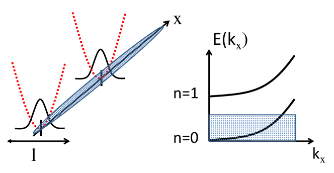
Figure 12: (left) Confinement of the electron gas in a one-dimensional tube of transverse size $l$. $x$ is the direction of the tube. Only one transverse direction of confinement has been shown for clarity. Due to the transverse confining potential the transverse degrees of freedom are strongly quantized. (right) Dispersion relation $E(k)$. Only half of the dispersion relation is shown for clarity. $k$ is the momentum parallel to the tube direction. The degrees of freedom transverse to the tube direction lead to the formation of minibands, labelled by a quantum number $n$. If only one miniband is populated, as represented by the gray box, the system is equivalent to a one dimensional system where only longitudinal degrees of freedom can vary.

The wavefunction of the system is thus of the form

$$\psi(x,r_{\perp})=e^{ikx}\phi(r_{\perp})$$ (86)

where $\phi$ depends on the precise form of the confining potential For an infinite well, as show in Fig. 12, $\phi$ is $\phi(y)=\sin((2n_{y}+1)\pi y/l)$, whereas it would be a gaussian function (49) for an harmonic confinement. The energy is of the form

$$E=\frac{k^{2}}{2m}+\frac{k_{y}^{2}}{2m}$$ (87)

where for simplicity I have taken hard walls confinement. Due to the narrowness of the transverse channel $l$, the quantization of $k_{y}$ is sizeable. Indeed, the change in energy by changing the transverse quantum number $n_{y}$ is at least (e.g. $n_{y}=0$ to $n_{y}=1$)

$$\Delta E=\frac{3\pi^{2}}{2ml^{2}}$$ (88)

This leads to minibands as shown in Fig. 12. If the distance between the minibands is larger than the temperature or interactions energy one is in a situation where only one miniband can be excited. The transverse degrees of freedom are thus frozen and only $k$ matters. The system is a one-dimensional quantum system.

2 Bosonization dictionary

Treating interacting particle in one dimension is a quite difficult task. One very interesting technique is provided by the so-called bosonization. It has the advantage of giving a very simple description of the low energy properties of the system, and of being completely general and very useful for many one dimensional systems. This chapter describe its vary basic features. For more details and physical insights on this technique both for fermions and bosons I refer the reader to [Giamarchi (2004)].

The idea behind the bosonization technique is to reexpress the excitations of the system in a basis of collective excitations. Indeed in one dimension it is easy to realize that single particle excitations cannot really exit. One particle when moving will push its neighbors and so on, which means that any individual motion is converted into a collective one. Collective excitations should thus be a good basis to represent a one dimensional system.

To exploit this idea, let us start with the density operator

$$\rho(x)=\sum_{i}\delta(x-x_{i})$$ (89)

where $x_{i}$ is the position operator of the $i$th particle. We label the position of the $i$th particle by an ‘equilibrium’ position $R_{i}^{0}$ that the particle would occupy if the particles were forming a perfect crystalline lattice, and the displacement $u_{i}$ relative to this equilibrium position. Thus,

$$x_{i}=R_{i}^{0}+u_{i}$$ (90)

If $\rho_{0}$ is the average density of particles, $d=\rho_{0}^{-1}$ is the distance between the particles. Then, the equilibrium position of the $i$th particle is

$$R_{i}^{0}=di$$ (91)

Note that at that stage it is not important whether we are dealing with fermions or bosons. The density operator written as (89) is not very convenient. To rewrite it in a more pleasant form we introduce a labelling field $\phi_{l}(x)$ [Haldane (1981a)]. This field, which is a continuous function of the position, takes the value $\phi_{l}(x_{i})=2\pi i$ at the position of the $i$th particle. It can thus be viewed as a way to number the particles. Since in one dimension, contrary to higher dimensions, one can always number the particles in an unique way (e.g. starting at $x=-\infty$ and processing from left to right), this field is always well-defined. Some examples are shown in Fig. 13.

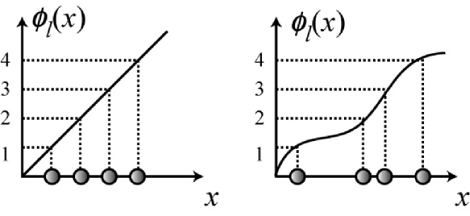
Figure 13: Some examples of the labelling field $\phi_{l}(x)$. If the particles form a perfect lattice of lattice spacing $d$, then $\phi_{l}^{0}(x)=2\pi x/d$, and is just a straight line. Different functions $\phi_{l}(x)$ allow to put the particles at any position in space. Note that $\phi(x)$ is always an increasing function regardless of the position of the particles. [From [Giamarchi (2004)]]

Using this labelling field and the rules for transforming $\delta$ functions

$$\delta(f(x))=\sum_{\mbox{zeros of $f$}}\frac{1}{|f^{\prime}(x_{i})|}\delta(x-x_{i})$$ (92)

one can rewrite the density as

$$\rho(x) = \sum_{i}\delta(x-x_{i})$$ (93)

$$= \sum_{n}|\nabla\phi_{l}(x)|\delta(\phi_{l}(x)-2\pi n)$$

It is easy to see from Fig. 13 that $\phi_{l}(x)$ can always be taken as an increasing function of $x$, which allows to drop the absolute value in (93). Using the Poisson summation formula this can be rewritten

$$\rho(x)=\frac{\nabla\phi_{l}(x)}{2\pi}\sum_{p}e^{ip\phi_{l}(x)}$$ (94)

where $p$ is an integer. It is convenient to define a field $\phi$ relative to the perfect crystalline solution and to introduce

$$\phi_{l}(x)=2\pi\rho_{0}x-2\phi(x)$$ (95)

The density becomes

$$\rho(x)=\left[\rho_{0}-\frac{1}{\pi}\nabla\phi(x)\right]\sum_{p}e^{i2p(\pi\rho_{0}x-\phi(x))}$$ (96)

Since the density operators at two different sites commute it is normal to expect that the field $\phi(x)$ commutes with itself. Note that if one averages the density over distances large compared to the interparticle distance $d$ all oscillating terms in (96) vanish. Thus, only $p=0$ remains and this smeared density is

$$\rho_{q\sim 0}(x)\simeq\rho_{0}-\frac{1}{\pi}\nabla\phi(x)$$ (97)

We can now write the single-particle creation operator $\psi^{\dagger}(x)$. Such an operator can always be written as

$$\psi^{\dagger}(x)=[\rho(x)]^{1/2}e^{-i\theta(x)}$$ (98)

where $\theta(x)$ is some operator. In the case where one would have Bose condensation, $\theta$ would just be the superfluid phase of the system. The commutation relations between the $\psi$ impose some commutation relations between the density operators and the $\theta(x)$. For bosons, the condition is

$$[\psi^{\phantom{\dagger}}_{B}(x),\psi_{B}^{\dagger}(x^{\prime})]=\delta(x-x^{\prime})$$ (99)

Using (98) the commutator gives

$$e^{+i\theta(x)}[\rho(x)]^{1/2}[\rho(x^{\prime})]^{1/2}e^{-i\theta(x^{\prime})}-[\rho(x^{\prime})]^{1/2}e^{-i\theta(x^{\prime})}e^{+i\theta(x)}[\rho(x)]^{1/2}$$ (100)

If we assume quite reasonably that the field $\theta$ commutes with itself ($[\theta(x),\theta(x^{\prime})]=0$), the commutator (100) is obviously zero for $x\neq x^{\prime}$ if (for $x\neq x^{\prime}$)

$$[[\rho(x)]^{1/2},e^{-i\theta(x^{\prime})}]=0$$ (101)

A sufficient condition to satisfy (99) would thus be

$$[\rho(x),e^{-i\theta(x^{\prime})}]=\delta(x-x^{\prime})e^{-i\theta(x^{\prime})}$$ (102)

It is easy to check that if the density were only the smeared density (97) then (102) is obviously satisfied if

$$[\frac{1}{\pi}\nabla\phi(x),\theta(x^{\prime})]=-i\delta(x-x^{\prime})$$ (103)

One can show that this is indeed the correct condition to use [Giamarchi (2004)]. Equation (103) proves that $\theta$ and $\frac{1}{\pi}\nabla\phi$ are canonically conjugate. Note that for the moment this results from totally general considerations and does not rest on a given microscopic model. Such commutation relations are also physically very reasonable since they encode the well known duality relation between the superfluid phase and the total number of particles. Integrating by part (103) shows that

$$\pi\Pi(x)=\hbar\nabla\theta(x)$$ (104)

where $\Pi(x)$ is the canonically conjugate momentum to $\phi(x)$.

To obtain the single-particle operator one can substitute (96) into (98). Since the square root of a delta function is also a delta function up to a normalization factor the square root of $\rho$ is identical to $\rho$ up to a normalization factor that depends on the ultraviolet structure of the theory. Thus,

$$\psi^{\dagger}_{B}(x)=[\rho_{0}-\frac{1}{\pi}\nabla\phi(x)]^{1/2}\sum_{p}e^{i2p(\pi\rho_{0}x-\phi(x))}e^{-i\theta(x)}$$ (105)

where the index $B$ emphasizes that this is the representation of a bosonic creation operator.

How to modify the above formulas if we have fermions instead of bosons? The density can obviously be expressed in the same way in terms of the field $\phi$. For the single-particle operator one has to satisfy an anticommutation relation instead of (99). We thus have to introduce in representation (98) something that introduces the proper minus sign when the two fermions operators are commuted. This is known as a Jordan–Wigner transformation. Here, the operator to add is easy to guess. Since the field $\phi_{l}$ has been constructed to be a multiple of $2\pi$ at each particle, $e^{i\frac{1}{2}\phi_{l}(x)}$ oscillates between $\pm 1$ at the location of consecutive particles. The Fermi field can thus be easily constructed from the boson field (98) by

$$\psi^{\dagger}_{F}(x)=\psi^{\dagger}_{B}(x)e^{i\frac{1}{2}\phi_{l}(x)}$$ (106)

This can be rewritten in a form similar to (98) as

$$\psi^{\dagger}_{F}(x)=[\rho_{0}-\frac{1}{\pi}\nabla\phi(x)]^{1/2}\sum_{p}e^{i(2p+1)(\pi\rho_{0}x-\phi(x))}e^{-i\theta(x)}$$ (107)

The above formulas are a way to represent the excitations of the system directly in terms of variables defined in the continuum limit.

The fact that all operators are now expressed in terms of variables describing collective excitations is at the heart of the use of such representation, since as already pointed out, in one dimension excitations are necessarily collective as soon as interactions are present. In addition the fields $\phi$ and $\theta$ have a very simple physical interpretation. If one forgets their canonical commutation relations, order in $\theta$ indicates that the system has a coherent phase as indicated by (105), which is the signature of superfluidity. On the other hand order in $\phi$ means that the density is a perfectly periodic pattern as can be seen from (96). This means that the system has “crystallized”. For fermions note that the least oscillating term in (107) corresponds to $p=\pm 1$. This leads to two terms oscillating with a period $\pm\pi\rho_{0}$ which is nothing but $\pm k_{\text{F}}$. These two terms thus represent the Fermions leaving around their respective Fermi points $\pm k_{\text{F}}$, also known as right movers and left movers.

3 Physical results and Luttinger liquid

To determine the Hamiltonian in the bosonization representation we use (105) in the kinetic energy of bosons. It becomes

$$H_{K}\simeq\int dx\frac{\hbar^{2}\rho_{0}}{2m}(\nabla e^{i\theta})(\nabla e^{-i\theta})=\int dx\frac{\hbar^{2}\rho_{0}}{2m}(\nabla\theta)^{2}$$ (108)

which is the part coming from the single-particle operator containing less powers of $\nabla\phi$ and thus the most relevant. Using (43) and (96), the interaction term becomes

$$H_{\rm int}=\int dxV_{0}\frac{1}{2\pi^{2}}(\nabla\phi)^{2}$$ (109)

plus higher order operators. Keeping only the above lowest order shows that the Hamiltonian of the interacting bosonic system can be rewritten as

$$H=\frac{\hbar}{2\pi}\int dx[\frac{uK}{\hbar^{2}}(\pi\Pi(x))^{2}+\frac{u}{K}(\nabla\phi(x))^{2}]$$ (110)

where I have put back the $\hbar$ for completeness. This leads to the action

$$S/\hbar=\frac{1}{2\pi K}\int dx\;d\tau[\frac{1}{u}(\partial_{\tau}\phi)^{2}+u(\partial_{x}\phi(x))^{2}]$$ (111)

This hamiltonian is a standard sound wave one. The fluctuation of the phase $\phi$ represent the “phonon” modes of the density wave as given by (96). One immediately sees that this action leads to a dispersion relation, $\omega^{2}=u^{2}k^{2}$, i.e. to a linear spectrum. $u$ is the velocity of the excitations. $K$ is a dimensionless parameter whose role will be apparent below. The parameters $u$ and $K$ are used to parameterize the two coefficients in front of the two operators. In the above expressions they are given by

$$\begin{split}uK&=\frac{\pi\hbar\rho_{0}}{m}\\ \frac{u}{K}&=\frac{V_{0}}{\hbar\pi}\end{split}$$ (112)

This shows that for weak interactions $u\propto(\rho_{0}V_{0})^{1/2}$ while $K\propto(\rho_{0}/V_{0})^{1/2}$. In establishing the above expressions we have thrown away the higher order operators, that are less relevant. The important point is that these higher order terms will not change the form of the Hamiltonian (like making cross terms between $\phi$ and $\theta$ appears etc.) but only renormalize the coefficients $u$ and $K$ (for more details see [Giamarchi (2004)]). For fermions it is easy to check that one obtains a similar form. The important difference is that since the single particle operator contains already $\phi$ and $\theta$ at the lowest order (see (107)) the kinetic energy alone leads to $K=1$ and interactions perturb around this value, while for bosons non-interacting bosons correspond to $K=\infty$.

The low-energy properties of interacting quantum fluids are thus described by an Hamiltonian of the form (110) provided the proper $u$ and $K$ are used. These two coefficients totally characterize the low-energy properties of massless one-dimensional systems. The bosonic representation and Hamiltonian (110) play the same role for one-dimensional systems than the Fermi liquid theory plays for higher-dimensional systems. It is an effective low-energy theory that is the fixed point of any massless phase, regardless of the precise form of the microscopic Hamiltonian. This theory, which is known as Luttinger liquid theory [Haldane (1981b), Haldane (1981a)], depends only on the two parameters $u$ and $K$. Provided that the correct value of these parameters are used, all asymptotic properties of the correlation functions of the system then can be obtained exactly using (96) and (105) or (107).

Computing the Luttinger liquid coefficient can be done very efficiently. For small interaction, perturbation theory such as (112) can be used. More generally one just needs two relations involving these coefficients to obtain them. These could be for example two thermodynamic quantities, which makes it easy to extract from either Bethe-ansatz solutions if the model is integrable or numerical solutions. The Luttinger liquid theory thus provides, coupled with the numerics, an incredibly accurate way to compute correlations and physical properties of a system (see e.g. [Klanjsek et al. (2008)] for a remarkable example). For more details on the various procedures and models see [Giamarchi (2004)]. But, of course, the most important use of Luttinger liquid theory is to justify the use of the boson Hamiltonian and fermion–boson relations as starting points for any microscopic model. The Luttinger parameters then become some effective parameters. They can be taken as input, based on general rules (e.g. for bosons $K=\infty$ for non interacting bosons and $K$ decreases as the repulsion increases, for other general rules see [Giamarchi (2004)]), without any reference to a particular microscopic model. This removes part of the caricatural aspects of any modelization of a true experimental system. This use of the Luttinger liquid is reminiscent of the one where perturbations (impurity, electron-phonon interactions etc.) are added on the Fermi liquid theory. The calculations in $d=1$ proceed in the same spirit with the Luttinger liquid replacing the Fermi liquid. The Luttinger liquid theory is thus an invaluable tool to tackle the effect of perturbations on an interacting one-dimensional electron gas (such as the effect of lattice, impurities, coupling between chains, etc.). I refer the reader to [Giamarchi (2004)] for more on those points.

4 Correlations

Let us now examine in details the physical properties of such a Luttinger liquid. For this we need the correlation functions. I briefly show here how to compute them using the standard operator technique. More detailed calculations and functional integral methods are given in [Giamarchi (2004)].

To compute the correlations we absorb the factor $K$ in the Hamiltonian by rescaling the fields (this preserves the commutation relation)

$$\phi=\sqrt{K}\quad,\quad\theta=\frac{1}{\sqrt{K}}\tilde{\theta}$$ (113)

The fields $\tilde{\phi}$ and $\tilde{\theta}$ can be expressed in terms of bosons operator $[b^{\phantom{\dagger}}_{q},b^{\dagger}_{q^{\prime}}]=\delta_{q,q^{\prime}}$. This ensures that their canonical commutation relations are satisfied. One has

$$\begin{split}\phi(x)&=-\frac{i\pi}{L}\sum_{p\neq 0}\left(\frac{L|p|}{2\pi}\right)^{1/2}\frac{1}{p}e^{-\alpha|p|/2-ipx}(b^{\dagger}_{p}+b^{\phantom{\dagger}}_{-p})\\ \theta(x)&=\frac{i\pi}{L}\sum_{p\neq 0}\left(\frac{L|p|}{2\pi}\right)^{1/2}\frac{1}{|p|}e^{-\alpha|p|/2-ipx}(b^{\dagger}_{p}-b^{\phantom{\dagger}}_{-p})\end{split}$$ (114)

where $L$ is the size of the system and $\alpha$ a short distance cutoff (of the order of the interparticle distance) needed to regularize the theory at short scales. The above expressions are in fact slightly simplified and zero modes should also be incorporated [Giamarchi (2004)]. This will not affect the remaining of this section and the calculation of the correlation functions.

It is easy to check by a direct substitution of (114) in (110) that Hamiltonian (110) with $K=1$ is simply

$$\tilde{H}=\sum_{p\neq 0}u|p|b^{\dagger}_{p}b^{\phantom{\dagger}}_{p}$$ (115)

The time (or imaginary time [Mahan (1981)]) dependence of the field can now be easily computed from (115) and (114). This gives

$$\phi(x,\tau)=-\frac{i\pi}{L}\sum_{p\neq 0}\left(\frac{L|p|}{2\pi}\right)^{1/2}\frac{1}{p}e^{-\alpha|p|/2-ipx}(b^{\dagger}_{p}e^{u|p|\tau}+b^{\phantom{\dagger}}_{-p}e^{-u|p|\tau})$$ (116)

and a similar expression for $\theta$. In order to compute physical observable we need to get correlations of exponentials of the fields $\phi$ and $\theta$. To do so one simply uses that for an operator $A$ that is linear in terms of boson fields and a quadratic Hamiltonian one has

$$\langle T_{\tau}e^{A}\rangle=e^{\frac{1}{2}\langle T_{\tau}A^{2}\rangle}$$ (117)

where $T_{\tau}$ is the time ordering operator. Thus, for example

$$\langle T_{\tau}e^{i2\phi(x,\tau)}e^{-i2\phi(0,0)}\rangle=e^{-2\langle T_{\tau}[\phi(x,\tau)-\phi(0,0)]^{2}\rangle}$$ (118)

Using these rules it is easy to compute the correlations [Giamarchi (2004)]. If we want to compute the fluctuations of the density

$$\langle T_{\tau}\rho(x,\tau)\rho(0)\rangle$$ (119)

we obtain, for bosons or fermions, using (96)

$$\langle T_{\tau}\rho(x,\tau)\rho(0)\rangle=\rho_{0}^{2}+\frac{K}{2\pi^{2}}\frac{y_{\alpha}^{2}-x^{2}}{(x^{2}+y_{\alpha}^{2})^{2}}+\rho_{0}^{2}A_{2}\cos(2\pi\rho_{0}x)\left(\frac{\alpha}{r}\right)^{2K}\\ +\rho_{0}^{2}A_{4}\;\cos(4\pi\rho_{0}x)\left(\frac{\alpha}{r}\right)^{8K}+\cdots$$ (120)

where $r=\sqrt{x^{2}+y^{2}}$ and $y=u\tau$. Here, the lowest distance in the theory is $\alpha\sim\rho_{0}^{-1}$. The amplitudes $A_{i}$ are non-universal objects. They depend on the precise microscopic model, and even on the parameters of the model. Contrary to the amplitudes $A_{n}$, which depend on the precise microscopic model, the power-law decay of the various terms are universal. They all depend on the unique Luttinger coefficient $K$. Physically the interpretation of the above formula is that the density of particles has fluctuations that can be sorted compared to the average distance between particles $\alpha\sim d=\rho_{0}^{-1}$. This is shown on Fig. 14.

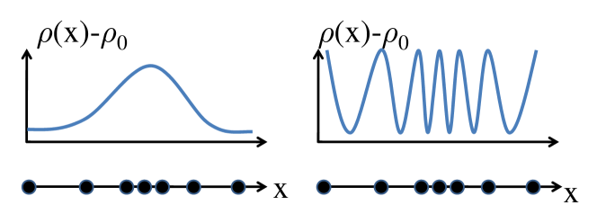
Figure 14: The density $\rho(x)$ can be decomposed in components varying with different Fourier wavevectors. The characteristic scale to separate these modes is the inter particle distance. Only the two lowest harmonics are represented here. Although they have very different spatial variations both these modes depends on the same smooth field $\phi(x)$. (left) the smooth variations of the density at lengthscale larger than the lattice spacing. These are simply $-\nabla\phi(x)/\pi$. (right) The density wave corresponding to oscillations of the density at a wavevector $Q=2\pi\rho_{0}$. These modes correspond to the operator $e^{i\pm 2\phi(x)}$.

The fluctuations of long wavelength decay with a universal power law. These fluctuations correspond to the hydrodynamic modes of the interacting quantum fluid. The fact that their fluctuation decay very slowly is the signature that there are massless modes present. This corresponds to the sound waves of density described by (110). However the density of particles has also higher fourier harmonics. The corresponding fluctuations also decay very slowly but this time with a non-universal exponent that is controlled by the LL parameter $K$. This is also the signature of the presence of a continuum of gapless modes, that exists for Fourier components around $Q=2n\pi\rho_{0}$ as shown in Fig. 14. For bosons $K$ goes to infinity when the interaction goes to zero which means that the correlations in the density decays increasingly faster with smaller interactions. This is consistent with the idea that the system becoming more and more superfluid smears more and more its density fluctuations. For fermions the noninteracting point corresponds to $K=1$ and one recovers the universal $1/r^{2}$ decay of the Friedel oscillations in a free electron gas. For repulsive interactions $K<1$ and density correlations decay more slowly, while for attractive interactions $K>1$ they will decay faster, being smeared by the superconducting pairing.

Let us now turn to the single particle correlation function

$$G(x,\tau)=-\langle T_{\tau}\psi(x,\tau)\psi^{\dagger}(0,0)\rangle$$ (121)

For bosons, at equal time this correlation function is a direct measure on whether a true condensate exists in the system. Its Fourier transform is the occupation factor $n(k)$. In presence of a true condensate, this correlation function tends to $G(x\to\infty,\tau=0)\to|\psi_{0}|^{2}$ the square of the order parameter $\psi_{0}=\langle\psi(x,\tau)\rangle$ when there is superfluidity. Its Fourier transform is a delta function at $q=0$, as shown in Fig. 15. In one dimension, no condensate can exist since it is impossible to break a continuous symmetry even at zero temperature, so this correlation must always go to zero for large space or time separation. Using (105) the correlation function can easily be computed. Keeping only the most relevant term ($p=0$) leads to (I have also put back the density result for comparison)

$$\begin{split}\langle T_{\tau}\psi(r)\psi^{\dagger}(0)\rangle&=A_{1}\left(\frac{\alpha}{r}\right)^{\frac{1}{2K}}+\cdots\\ \langle T_{\tau}\rho(r)\rho(0)\rangle&=\rho_{0}^{2}+\frac{K}{2\pi^{2}}\frac{y_{\alpha}^{2}-x^{2}}{(y_{\alpha}^{2}+x^{2})^{2}}+A_{3}\cos(2\pi\rho_{0}x)\left(\frac{1}{r}\right)^{2K}+\cdots\end{split}$$ (122)

where the $A_{i}$ are the non-universal amplitudes. For the non-interacting system $K=\infty$ and we recover that the system possesses off-diagonal long-range order since the single-particle Green’s function does not decay with distance. The system has condensed in the $q=0$ state. As the repulsion increases ($K$ decreases), the correlation function decays faster and the system has less and less tendency towards superconductivity. The occupation factor $n(k)$ has thus no delta function divergence but a power law one, as shown in Fig. 15.

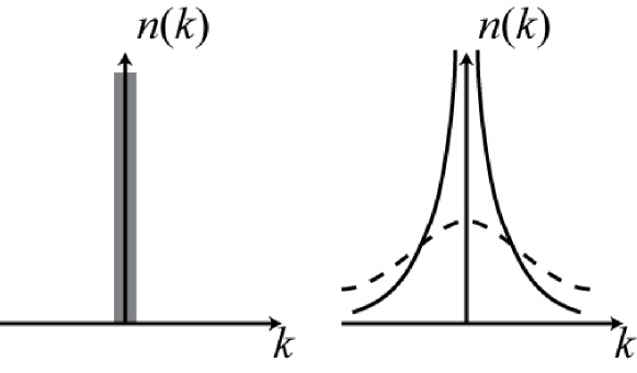
Figure 15: Momentum distribution $n(k)$ for the bosons as a function of the momentum $k$. (left) For non-interacting bosons all bosons are in $k=0$ state, thus $n(k)\propto\delta(k)$ (thick line). (right) As soon as interactions are introduced a true condensate cannot exist. The $\delta$ function is replaced by a power law divergence with an exponent $\nu=1-1/(2K)$ (solid line). At finite temperature, the superfluid correlation functions decay exponentially leading to a rounding of the divergence and a lorentzian like shape for $n(k)$. This is indicated by the dashed line.

Note that the presence of the condensate or not is not directly linked to the question of superfluidity. The fact that the system is a Luttinger liquid with a finite velocity $u$, implies that in one dimension an interacting boson system has always a linear spectrum $\omega=uk$, contrary to a free boson system where $\omega\propto k^{2}$. Such a system is thus a true superfluid at $T=0$ since superfluidity is the consequence of the linear spectrum [Mikeska and Schmidt (1970)]. Of course when the interaction tends to zero $u\to 0$ as it should to give back the quadratic dispersion of free bosons.

For fermions the single particle correlation function contains the terms $p=\pm 1$, corresponding to fermions close to $\pm k_{\text{F}}$ respectively. If we compute the correlation for the right movers we get

$$\begin{split}G_{R}(x,\tau)&=-e^{ik_{\text{F}}x}\langle T_{\tau}e^{i(\theta(x,\tau)-\phi(x,\tau)}e^{-i(\theta(0,0)-\phi(0,0))}\rangle\\ &=e^{ik_{\text{F}}x}e^{-[\frac{K+K^{-1}}{2}\log(r/\alpha)-i{\rm Arg}(y+ix)]}\end{split}$$ (123)

The single particle correlation thus decays as a non-universal power law whose exponent depends on the Luttinger liquid parameter. For free particles ($K=1$) one recovers

$$G_{R}(r)=-e^{ik_{\text{F}}x}e^{-\log[(y_{\alpha}-ix)/\alpha]}=-ie^{ik_{\text{F}}x}\frac{1}{x+i(v_{F}\tau+\alpha\;{\rm Sign}(\tau))}$$ (124)

which is the normal function for ballistic particles with velocity $u$. For interacting systems $K\neq 1$ the decay of the correlation is always faster, which shows that single particle excitations do not exist in the one dimensional world. One important consequence is the occupation factor $n(k)$ which is given by the Fourier transform of the equal time Green’s function

$$n(k)=\int dx\;e^{-ikx}G_{R}(x,0^{-})=-\int dx\;e^{i(k_{\text{F}}-k)x}\left(\frac{\alpha}{\sqrt{x^{2}+\alpha^{2}}}\right)^{\frac{K+K^{-1}}{2}}e^{i\;{\rm Arg}(-\alpha+ix)}$$ (125)

The integral can be easily determined by simple dimensional analysis. It is the Fourier transform of a power law and thus

$$n(k)\propto|k-k_{\text{F}}|^{\frac{K+K^{-1}}{2}-1}$$ (126)

The occupation factor is shown in Fig. 16.

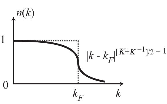
Figure 16: The occupation factor $n(k)$. Instead of the usual discontinuity at $k_{\text{F}}$ for a Fermi liquid, it has a power law essential singularity. This is the signature that fermionic quasiparticles do not exist in one dimension. Note that the position of the singularity is still at $k_{\text{F}}$. This is a consequence of Luttinger’s theorem stating that the volume of the Fermi surface cannot be changed by interactions.

Instead of the discontinuity at $k_{\text{F}}$ that signals in a Fermi liquid that fermionic quasiparticles are sharp excitations, one thus finds in one dimension an essential power law singularity. Formally, this corresponds to $Z=0$, another signature that all excitations are converted to collective excitations and that new physics emerges compared to the Fermi liquid case.

5 Conclusions

This concludes this brief tour of interacting quantum fluids. Of course we have just scratched the surface in these notes. The problem is an active research field, with extensive efforts both on the theoretical and the experimental point of view.

The Fermi liquid concept is still one of the cornerstone of our understanding of such systems, and is certainly the reference on which all novel properties must be compared. Models allowing to deal with interactions are still resisting our best attempts to fully solve them and in particular the Hubbard model, after about 50 years still remains a challenge, in particular in two dimensions. Cold atomic systems in optical lattices have provided a remarkable realization of such models and it is certain that the stimulation of those novel experimental realization should help driving the field forward.

Last but not least the one dimensional world, with its own properties and challenges is now at a stage where it has the corresponding concept of the Fermi liquid, the so called Luttinger liquid. This allows to move forward and understand the effects of various perturbations, such as lattice, disorder, effect of coupling of one dimensional chains, which are at the heart of the several realization of the one dimensional systems that we have today. We thus see that the one dimensional world can be connected by that route to its higher dimensional counterpart, and might also provide a way to tackle it. Considerable development can thus be expected in the coming years.

6 Acknowledgements

The research described in this work was supported in part by the Swiss NSF under MaNEP and Division II.

References

- Abrikosov et al. (1963) Abrikosov, A. A., Gorkov, L. P., and Dzyaloshinski, I. E. (1963). Methods of Quantum Field Theory in Statistical Physics. Dover, New York.
- Anderson (1959) Anderson, P. W. (1959). Phys. Rev., 115, 2.
- Andres et al. (1975) Andres, K., Graebner, J. E., and Ott, H. R. (1975). Physical Review Letters, 35, 1779.
- Anglin and Ketterle (2002) Anglin, J. R. and Ketterle, W. (2002). Nature (London), 416, 211.
- Ashcroft and Mermin (1976) Ashcroft, N. W. and Mermin, N. D. (1976). Solid State Physics. Saunders College, Philadelphia.
- Auerbach (1998) Auerbach, A. (1998). Interacting Electrons and Quantum Magnetism. Springer, Berlin.
- Berg et al. (2009) Berg, Erez, Dalla Torre, Emanuele G., Giamarchi, Thierry, and Altman, Ehud (2009). Phys. Rev. B, 77, 245119.
- Bloch et al. (2008) Bloch, I., Dalibard, J., and Zwerger, W. (2008). Rev. Mod. Phys., 80, 885.
- Brinkman and Rice (1970) Brinkman, W. F. and Rice, T. M. (1970). Phys. Rev. B, 2, 4302.
- Dagotto and Rice (1996) Dagotto, E. and Rice, T. M. (1996). Science, 271, 5249.
- Damascelli et al. (2003) Damascelli, A., Hussain, Z., and Shen, Z.-X. (2003). Rev. Mod. Phys., 75, 473.
- Dresselhaus et al. (1995) Dresselhaus, M. S., Dresselhaus, G., and Eklund, P. C. (1995). Science of Fullerenes and Carbon Nanotubes. Academic Press, San Diego, CA.
- Duan et al. (2003) Duan, L.-M., Demler, E., and Lukin, M. D. (2003). Physical Review Letters, 91, 090402.
- Fazio and van der Zant (2001) Fazio, R. and van der Zant, H. (2001). Phys. Rep., 355, 235.
- Fisher and Glazman (1997) Fisher, M. P. A. and Glazman, L. I. (1997). In Mesoscopic Electron Transport (ed. L. Kowenhoven et al.), Dordrecht. Kluwer Academic Publishers. cond-mat/9610037.
- Fisher et al. (1989) Fisher, M. P. A., Weichman, P. B., Grinstein, G., and Fisher, D. S. (1989). Phys. Rev. B, 40, 546.
- Giamarchi (2004) Giamarchi, Thierry (2004). Quantum Physics in one Dimension. Volume 121, International series of monographs on physics. Oxford University Press, Oxford, UK.
- Giamarchi et al. (2008) Giamarchi, T., Ruegg, C., and Tchernyshyov, O. (2008). Nature Physics, 4, 198.
- Greiner et al. (2002) Greiner, M., Mandel, O., Esslinger, T., Hänsch, T. W., and Bloch, I. (2002). Nature, 415, 39.
- Greywall (1983) Greywall, D. S. (1983). Phys. Rev. B, 27, 2747.
- Greywall (1984) Greywall, D. S. (1984). Phys. Rev. B, 29, 4933.
- Gutzwiller (1965) Gutzwiller, M. C. (1965). Phys. Rev., 137, A1726.
- Haldane (1981a) Haldane, F. D. M. (1981a). Physical Review Letters, 47, 1840.
- Haldane (1981b) Haldane, F. D. M. (1981b). Journal of Physics C, 14, 2585.
- Haldane (1981c) Haldane, F. D. M. (1981c). Physical Review Letters, 47, 1840.
- Haldane (1983) Haldane, F. D. M. (1983). Physical Review Letters, 50, 1153.
- Ho et al. (2009) Ho, A. F., Cazalilla, M. A., and Giamarchi, T. (2009). Phys. Rev. A, 79, 033620.
- Imada et al. (1998) Imada, M., Fujimori, A., and Tokura, Y. (1998). Rev. Mod. Phys., 70, 1039.
- Jaksch et al. (1998) Jaksch, D., Bruder, C., Cirac, J. I., Gardiner, C. W., and Zoller, P. (1998). Physical Review Letters, 81, 3108.
- Klanjsek et al. (2008) Klanjsek et al., M. (2008). Physical Review Letters, 101, 137207.
- Kotliar and Ruckenstein (1986) Kotliar, Gabriel and Ruckenstein, Andrei E. (1986). Physical Review Letters, 57(11), 1362.
- Kotliar and Vollhardt (2004) Kotliar, G. and Vollhardt, D. (2004). Physics Today, 57, 53.
- Landau (1957a) Landau, L. D. (1957a). Sov. Phys. JETP, 3, 920.
- Landau (1957b) Landau, L. D. (1957b). Sov. Phys. JETP, 5, 101.
- Lebed (2007) Lebed, A. (ed.) (2007). The Physics of Organic Superconductors. Springer.
- Mahan (1981) Mahan, G. D. (1981). Many Particle Physics. Plenum, New York.
- Matsubara and Matsuda (1956) Matsubara, T. and Matsuda, H. (1956). Progess of Theoretical Physics, 16, 569.
- Mikeska and Schmidt (1970) Mikeska, H. J. and Schmidt, H. (1970). J. Low Temp. Phys, 2, 371.
- Mott (1949) Mott, N. F. (1949). Proc. Phys. Soc. Sect. A, 62, 416.
- Niyaz et al. (1994) Niyaz, P., Scalettar, R. T., Fong, C. Y., and Batrouni, G. G. (1994). Phys. Rev. B.
- Nozieres (1961) Nozieres, P. (1961). Theory of Interacting Fermi systems. W. A. Benjamin, New York.
- Pitaevskii and Stringari (2003) Pitaevskii, L. and Stringari, S. (2003). Bose-Einstein Condensation. Clarendon Press, Oxford.
- Stöferle et al. (2004) Stöferle, T., Moritz, H., Schori, C., Köhl, M., and Esslinger, T. (2004). Physical Review Letters, 92, 130403.
- Valla et al. (1999) Valla, T., Fedorov, A. V., Johnson, P. D., and Hulbert, S. L. (1999). Physical Review Letters, 83, 2085.
- Wen (1995) Wen, X. G. (1995). Advances In Physics, 44, 405.
- Wessel and Troyer (2005) Wessel, Stefan and Troyer, Matthias (2005). Physical Review Letters, 95, 127205.
- Yokoyama and Shiba (1987) Yokoyama, H. and Shiba, H. (1987). J. Phys. Soc. Jpn., 56, 3582.
- Ziman (1972) Ziman, J. M. (1972). Principles of the Theory of Solids. Cambridge University Press, Cambridge.
- Zvonarev et al. (2007) Zvonarev, M., Cheianov, V. V., and Giamarchi, T. (2007). Physical Review Letters, 99, 240404.
- Zwerger (2003) Zwerger, W. (2003). J. Opt. B: Quantum Semiclass. Opt., 5, 9.