Probabilistic initial value problem for cellular automaton rule 172

Abstract

We present a method of solving of the probabilistic initial value problem for cellular automata (CA) using CA rule 172 as an example. For a disordered initial condition on an infinite lattice, we derive exact expressions for the density of ones at arbitrary time step. In order to do this, we analyze topological structure of preimage trees of finite strings of length 3. Level sets of these trees can be enumerated directly using classical combinatorial methods, yielding expressions for the number of $n$-step preimages of all strings of length 3, and, subsequently, probabilities of occurrence of these strings in a configuration obtained from the initial one after $n$ iterations of rule 172. The density of ones can be expressed in terms of Fibonacci numbers, while expressions for probabilities of other strings involve Lucas numbers. Applicability of this method to other CA rules is briefly discussed.

1 Introduction

While working on a certain problem in complexity engineering, that is, trying to construct a cellular automaton rule performing some useful computational task, the author encountered the following question. Let $f:\{0,1\}^{3}\to\{0,1\}$ be defined as

$$f(x_{1},x_{2},x_{3})=\left\{\begin{array}[]{ll}x_{2}&\mbox{if $x_{1}=0$,}\\ x_{3}&\mbox{if $x_{1}=1$.}\end{array}\right.$$ (1)

This function may be called selective copier, since it returns (copies) one of its inputs $x_{2}$ or $x_{3}$ depending on the state of the first input variable $x_{1}$. Suppose now that $s$ be a bi-infinite sequence of binary symbols, i.e., $s=\ldots s_{-2}s_{-1}s_{0}s_{1}s_{2}\ldots$, $i\in{\mathbbm{Z}}$. We will transform this string using the selective copier, that is, for each $i$, we keep $s_{i}$ if it is preceded by $0$, or replace it by $s_{i+1}$ otherwise, so that each $s_{i}$ is simultaneously replaced by $f(s_{i-1},s_{i},s_{i+1})$. Consider now the question: Assuming that the initial sequence is randomly generated, what is the proportion of 1’s in the sequence after $n$ iterations of the aforementioned procedure?

Function defined by eq. (1) is a local function of cellular automaton rule 172, using Wolfram numbering, and the aforementioned question is an example of a broader class of problems, which could be called probabilistic initial value problems for cellular automata: given initial distribution of infinite configurations, what is the probability of occurrence of a given finite string in a configuration obtained from the initial one by $n$ iterations of the cellular automaton rule? In what follows, we will demonstrate how one can approach probabilistic initial value problem using cellular automaton rule 172 as an example.

2 Basic definitions

Let ${\mathcal{G}}=\{0,1,...N-1\}$ be called a symbol set, and let ${\mathcal{S}}({\mathcal{G}})$ be the set of all bisequences over ${\mathcal{G}}$, where by a bisequence we mean a function on ${\mathbbm{Z}}$ to ${\mathcal{G}}$. Set ${\mathcal{S}}({\mathcal{G}})$ will be called the configuration space. Throughout the remainder of this text we shall assume that ${\mathcal{G}}=\{0,1\}$, and the configuration space ${\mathcal{S}}({\mathcal{G}})=\{0,1\}^{{\mathbbm{Z}}}$ will be simply denoted by ${\mathcal{S}}$.

A block of length $n$ is an ordered set $b_{0}b_{1}\ldots b_{n-1}$, where $n\in{\mathbbm{N}}$, $b_{i}\in{\mathcal{G}}$. Let $n\in{\mathbbm{N}}$ and let ${\mathcal{B}}_{n}$ denote the set of all blocks of length $n$ over ${\mathcal{G}}$ and ${\mathcal{B}}$ be the set of all finite blocks over ${\mathcal{G}}$.

For $r\in{\mathbbm{N}}$, a mapping $f:\{0,1\}^{2r+1}\mapsto\{0,1\}$ will be called a cellular automaton rule of radius $r$. Alternatively, the function $f$ can be considered as a mapping of ${\mathcal{B}}_{2r+1}$ into ${\mathcal{B}}_{0}={\mathcal{G}}=\{0,1\}$.

Corresponding to $f$ (also called a local mapping) we define a global mapping $F:{\mathcal{S}}\to{\mathcal{S}}$ such that $(F(s))_{i}=f(s_{i-r},\ldots,s_{i},\ldots,s_{i+r})$ for any $s\in{\mathcal{S}}$.

A block evolution operator corresponding to $f$ is a mapping ${\mathbf{f}}:{\mathcal{B}}\mapsto{\mathcal{B}}$ defined as follows. Let $r\in{\mathbbm{N}}$ be the radius of $f$, and let $a=a_{0}a_{1}\ldots a_{n-1}\in{\mathcal{B}}_{n}$ where $n\geq 2r+1>0$. Then

$${\mathbf{f}}(a)=\{f(a_{i},a_{i+1},\ldots,a_{i+2r})\}_{i=0}^{n-2r-1}.$$ (2)

Note that if $b\in B_{2r+1}$ then $f(b)={\mathbf{f}}(b)$.

We will consider the case of ${\mathcal{G}}=\{0,1\}$ and $r=1$ rules, i.e., elementary cellular automata. In this case, when $b\in{\mathcal{B}}_{3}$, then $f(b)={\mathbf{f}}(b)$. The set ${\mathcal{B}}_{3}=\{000,001,010,011,100,101,101,110$, $111\}$ will be called the set of basic blocks.

The number of $n$-step preimages of the block $b$ under the rule $f$ is defined as the number of elements of the set ${\mathbf{f}}^{-n}(b)$. Given an elementary rule $f$, we will be especially interested in the number of $n$-step preimages of basic blocks under the rule $f$.

3 Probabilistic initial value problem

The appropriate mathematical description of an initial distribution of configurations is a probability measure $\mu$ on ${\mathcal{S}}$. Such a measure can be formally constructed as follows. If $b$ is a block of length $k$, i.e., $b=b_{0}b_{1}\ldots b_{k-1}$, then for $i\in{\mathbbm{Z}}$ we define a cylinder set. The cylinder set is a set of all possible configurations with fixed values at a finite number of sites. Intuitively, measure of the cylinder set given by the block $b=b_{0}\ldots b_{k-1}$, denoted by $\mu[C_{i}(b)]$, is simply a probability of occurrence of the block $b$ in a place starting at $i$. If the measure $\mu$ is shift-invariant, than $\mu(C_{i}(b))$ is independent of $i$, and we will therefore drop the index $i$ and simply write $\mu(C(b))$.

The Kolmogorov consistency theorem states that every probability measure $\mu$ satisfying the consistency condition

$$\mu[C_{i}(b_{1}\ldots b_{k})]=\mu[C_{i}(b_{1}\ldots b_{k},0)]+\mu[C_{i}(b_{1}\ldots b_{k},1)]$$ (3)

extends to a shift invariant measure on $\cal S$ (Dynkin, 1969) .For $p\in[0,1]$, the Bernoulli measure defined as $\mu_{p}[C(b)]=p^{j}(1-p)^{k-j}$, where $j$ is a number of ones in $b$ and $k-j$ is a number of zeros in $b$, is an example of such a shift-invariant (or spatially homogeneous) measure. It describes a set of random configurations with the probability $p$ that a given site is in state $1$.

Since a cellular automaton rule with global function $F$ maps a configuration in ${\mathcal{S}}$ to another configuration in ${\mathcal{S}}$, we can define the action of $F$ on measures on ${\mathcal{S}}$. For all measurable subsets $E$ of ${\mathcal{S}}$ we define $(F\mu)(E)=\mu(F^{-1}(E))$, where $F^{-1}(E)$ is an inverse image of $E$ under $F$.

If the initial configuration was specified by $\mu_{p}$, what can be said about $F^{n}\mu_{p}$ (i.e., what is the probability measure after $n$ iterations of $F$)? In particular, given a block $b$, what is the probability of the occurrence of this block in a configuration obtained from a random configuration after $n$ iterations of a given rule?

The general question of finding the iterrates of the Bernoulli measure under a given CA has been extensively studied in recent years by many authors, including, among others, Lind (1984); Ferrari et al. (2000); Maass and Martínez (2003); Host et al. (2003); Pivato and Yassawi (2002, 2004); Maass et al. (2006) and Maass et al. (2006). In this paper, we will approach the problem from somewhat different angle, using very elementary methods and without resorting to advanced apparatus of ergodic theory and symbolic dynamics. We will consider iterates of the Bernoulli measure by analyzing patterns in preimage sets.

For a given block $b$, the set of $n$-step preimages is ${\mathbf{f}}^{-n}(b)$. Then, by the definition of the action of $F$ on the initial measure, we have

$$(F^{n}\mu_{p})(C(b))=\mu_{p}\left(F^{-n}(C(b))\right),$$ (4)

and consequently

$$(F^{n}\mu_{p})(C(b))=\sum_{a\in{\mathbf{f}}^{-n}(b)}\mu_{p}(a).$$ (5)

Let us define the probability of occurrence of block $b$ in a configuration obtained from the initial one by $n$ iterations of the CA rule as

$$P_{n}(b)=(F^{n}\mu_{p})(C(b)).$$ (6)

Using this notation, eq. (5) becomes

$$P_{n}(b)=\sum_{a\in{\mathbf{f}}^{-n}(b)}P_{0}(a).$$ (7)

If the initial measure is $\mu_{1/2}$, then all blocks of a given length are equally probable, and $P_{0}(a)=\frac{1}{2^{|a|}}$, where $|a|$ is the length of the block $a$. For elementary CA rule, the length of $n$-step preimage of $b$ is $2n+|b|$, therefore

$$P_{n}(b)=2^{-|b|-2n}\mathop{\mathrm{card}}{\mathbf{f}}^{-n}(b).$$ (8)

This equation tells us that if the initial measure is symmetric ($\mu_{1/2}$), then all we need to know in order to compute $P_{n}(b)$ is the cardinality of ${\mathbf{f}}^{-n}(b)$. One way to think about this is to draw a preimage tree for $b$. We start form $b$ as a root of the tree, and determine all its preimages. Then each of these preimages is connected with $b$ by an edge. They constitute level 1 of the preimage tree. Then, for each block of level 1, we again compute its preimages and we link them with that block, thus obtaining level 2. Repeating this operation ad infinitum, we obtain a tree such as the one shown in Figure 1. In that figure, five levels of the preimage tree for rule 172 rooted at $101$ are shown, with only first level labelled.

Note that $\mathop{\mathrm{card}}{\mathbf{f}}^{-n}(b)$ corresponds to the number of vertices in the $n$-th level of the preimage tree. One thus only needs to know cardinalities of level sets in order to use eq. (8), while the exact topology of connections between vertices of the preimage tree is unimportant.

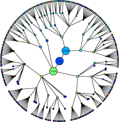
Figure 1: Preimage tree for rule 172 rooted at $101$.

The key problem, therefore, is to enumerate level sets. In order to answer the question posed in the introduction, we need to compute $P_{n}(1)$ for rule 172, which, in turn, requires that we enumerate level sets of a preimage tree rooted at $1$. It turns out that for rule 172 the preimage tree rooted at 1 is rather complicated, and that it is more convenient to consider preimage trees rooted at other blocks. In the next section, we will show how to express $P_{n}(1)$ by some other block probabilities. From now on, ${\mathbf{f}}$ will exclusively denote the block evolution operator for rule 172.

4 Block probabilities

Since ${\mathbf{f}}^{-1}(1)=\{010,011,101,111\}$, we have $P_{n+1}(1)=P_{n}(010)+P_{n}(011)+P_{n}(101)+P_{n}(111)$. Due to consistency conditions (eq. 3), $P_{n}(010)+P_{n}(011)=P_{n}(01)$, and we obtain

$$P_{n+1}(1)=P_{n}(01)+P_{n}(101)+P_{n}(111).$$ (9)

This can be transformed even further by noticing that $P_{n}(01)=P_{n}(001)+P_{n}(101)$, therefore

$$P_{n}(1)=P_{n-1}(001)+2P_{n-1}(101)+P_{n-1}(111).$$ (10)

By using eq. (8) and defining $c_{n}=P_{n}(1)$ we obtain

$$c_{n}=\frac{\mathop{\mathrm{card}}{\mathbf{f}}^{-n+1}(001)+2\mathop{\mathrm{card}}{\mathbf{f}}^{-n+1}(101)+\mathop{\mathrm{card}}{\mathbf{f}}^{-n+1}(111)}{2^{2n+1}}.$$ (11)

This means that in order to compute $c_{n}$, we need to know cardinalities of $n$-step preimages of 001, 101, and 111.

5 Structure of preimage sets

The structure of level sets of preimage trees rooted at $001$, $101$, and $111$ will be described in the following three propositions.

Proposition 5.1

Block $b$ belongs to ${\mathbf{f}}^{-n}(001)$ if and only if it has the structure

$$b=\underbrace{\star\star\ldots\star}_{n}001\underbrace{\star\star\ldots\star}_{n},$$ (12)

where $\star$ represents arbitrary symbol from the set $\{0,1\}$.

Let us first observe that ${\mathbf{f}}^{-1}(001)=\{00010,00011,10010,10011\}$, which means that ${\mathbf{f}}^{-1}(001)$ can be represented as $\star\star 001\star\star$. Similarly, therefore, ${\mathbf{f}}^{-2}(001)$ has the structure $\star\star\star 001\star\star\star$, and by induction, for any $n$, the structure of ${\mathbf{f}}^{-n}(001)$ must be $\underbrace{\star\star\ldots\star}_{n}001\underbrace{\star\star\ldots\star}_{n}$. $\Box$

Proposition 5.2

Block $b$ belongs to ${\mathbf{f}}^{-n}(101)$ if and only if it has the structure

$$b=\underbrace{\star\star\ldots\star}_{n-1}a_{1}a_{2}\ldots a_{n}1101,$$ (13)

where $a_{i}\in\{0,1\}$ for $i=1,\ldots,n$ and the string $a_{1}a_{2}\ldots a_{n}$ does not contain any pair of adjacent zeros, that is. $a_{i}a_{i+1}\neq 00$ for all $i=1,\ldots,n-1$.

Two observations will be crucial for the proof. First of all, ${\mathbf{f}}^{-1}(101)=\{01101,11101\}$, thus ${\mathbf{f}}^{-1}(101)$ has the structure $\star 1101$. Furthermore, we have ${\mathbf{f}}^{-1}(1101)=\{011101,101101,111101\}$, meaning that if $1101$ appears in a configuration, and is not preceded by $00$, then after application of the rule 172, $1101$ will still appear, but shifted one position to the left. All this means that if $b$ is to be an $n$-step preimage of $101$, it must end with $1101$. After each application of rule 172 to $b$, the block $1101$ will remain at the end as long as it is not preceded by two zeros.

Now, let us note that ${\mathbf{f}}^{-1}(00)=\{0000,0001,1000,1001,1100\}$, which means that preimage of $00$ is either $1100$ or $\star 00\star$. Therefore, we can say that if $00$ is not present in the string $a_{1}a_{2}\ldots a_{n}$, it will not appear in its consecutive images under ${\mathbf{f}}$. Thus, block $1101$ will, after each iteration of $f$, remain at the end, and will never be preceded by two zeros. Eventually, after $n$ iterations, it will produce $101$, as shown in the example below.

$$\begin{array}[]{lllllllllllll}1&0&1&0&0&1&1&1&0&\textbf{1}&\textbf{1}&\textbf{0}&\textbf{1}\\ &1&1&0&0&1&1&0&\textbf{1}&\textbf{1}&\textbf{0}&\textbf{1}&\\ &&0&0&0&1&0&\textbf{1}&\textbf{1}&\textbf{0}&\textbf{1}&&\\ &&&0&0&1&\textbf{1}&\textbf{1}&\textbf{0}&\textbf{1}&&&\\ &&&&0&\textbf{1}&\textbf{1}&\textbf{0}&\textbf{1}&&&&\\ &&&&&1&0&1&&&&&\end{array}$$

What is left to show is that not having $00$ in $a_{1}a_{2}\ldots a_{n}$ is necessary. This is a consequence of the fact that ${\mathbf{f}}(\star 00\star)=00$, which means that if $00$ appears in a string, then it stays in the same position after the rule 172 is applied. Indeed, if we had a pair of adjacent zeros in $a_{1}a_{2}\ldots a_{n}$, it would stay in the same position when ${\mathbf{f}}$ is applied, and sooner or later block $1101$, which is moving to the left, would come to the position immediately following this pair, and would be destroyed in the next iteration, thus never producing $101$. Such a process is illustrated below, where after three iterations the block $1101$ is destroyed due to “collision” with $00$. $\Box$

$$\begin{array}[]{lllllllllllll}1&0&1&0&0&0&1&1&0&\textbf{1}&\textbf{1}&\textbf{0}&\textbf{1}\\ &1&1&0&0&0&1&0&\textbf{1}&\textbf{1}&\textbf{0}&\textbf{1}&\\ &&0&0&0&0&1&\textbf{1}&\textbf{1}&\textbf{0}&\textbf{1}&&\\ &&&0&0&0&\textbf{1}&\textbf{1}&\textbf{0}&\textbf{1}&&&\\ &&&&0&0&1&0&1&&&&\\ &&&&&0&1&1&&&&&\end{array}$$

Proposition 5.3

Block $b$ belongs to ${\mathbf{f}}^{-n}(111)$ if and only if it has the structure

$$b=\underbrace{\star\star\ldots\star}_{n-2}a_{1}a_{2}\ldots a_{n+5},$$ (14)

where $a_{i}\in\{0,1\}$ for $i=1,\ldots,n$ and the string $a_{1}a_{2}\ldots a_{n}$ satisfies the following three conditions:

• $a_{i}a_{i+1}\neq 00$ for all $i=2\ldots n+4$;

• $a_{n+3}a_{n+4}a_{n+5}\neq 110$ and $a_{n+2}a_{n+3}a_{n+4}\neq 110$;

• if $a_{1}a_{2}\neq 00$, then $a_{n+1}a_{n+2}a_{n+3}\neq 110$.

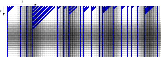
Figure 2: Example of a spatiotemporal pattern produced by rule 172.

We will present only the main idea of the proof here, omitting some tedious details. It will be helpful to inspect spatiotemporal pattern generated by rule 172 first, as shown in Figure 2. Careful inspection of this pattern reveals three facts, each of them easily provable in a rigorous way:

• A cluster of two or more zeros keeps its right boundary in the same place for ever.

• A cluster of two or more zeros extends its left boundary to the left one unit per time step as long as the left boundary is preceded by two or more ones. If the left boundary it is preceded by 01, it stays in the same place.

• Isolated zero moves to the left one step at a time as long as it has at least two ones on the left. If an isolated zero is preceded by 10, it disappears in the next time step.

Let us first prove that (i)-(iii) are necessary. Condition (i) is needed because if we had $00$ in the string $a_{2}\ldots a_{n+5}$, its left boundary would grow to the left and after $n$ iterations it would reach sites in which we expect to find the resulting string $111$.

Moreover, string $a_{1}a_{2}\ldots a_{n+5}$ cannot have $011$ at the end position, one site before the end, or two sites before the end. If it had, 0 preceded by two 1’s would move to the left and, after $n$ iterations, it would reach sites where we want to find $111$. The only exception to this is the case when $a_{0}a_{1}=00$. In this case, even if $011$ is in the second position from the end, it will disappear in step $n-1$. This demonstrates that (ii) and (iii) are necessary.

In order to prove sufficiency of (i)-(iii), let us suppose that the string $b$ satisfies all these conditions yet ${\mathbf{f}}^{n}(b)\neq 111$. This would imply that at least one of the symbols of ${\mathbf{f}}^{n}(b)$ is equal to zero. However, according to what we stated in F1–F3, zero can appear in a later configuration only as a result of growth of an initial cluster of two of more zeros, or by moving to the left if it is preceded by two ones. This, however, is impossible due to conditions (i)-(iii). $\Box$.

6 Enumeration of preimage strings

Once we know the structure of preimage sets, we can enumerate them. For this, the following lemma will be useful.

Lemma 6.1

The number of binary strings $a_{1}a_{2}\ldots a_{n}$ such that $00$ does not appear as two consecutive terms $a_{i}a_{i+1}$ is equal to $F_{n+2}$, where $F_{n}$ is the $n$-th Fibonacci number.

This result will be derived using classical transfer-matrix method. Let $g(n)$ be the number of binary strings $a_{1}a_{2}\ldots a_{n}$ such that $00$ does not appear as two consecutive terms $a_{i}a_{i+1}$. We can think of such string as a walk of length $n$ on a graph with vertices $v_{1}=0$ and $v_{2}=1$ which has adjacency matrix $A$ given by $A_{11}=0$, $A_{12}=A_{21}=A_{22}=1$. One can prove that the generating function for $g$,

$$G(\lambda)=\sum_{n=0}^{\infty}g(n+1)\lambda^{n},$$ (15)

can be expressed by $G(\lambda)=G_{11}(\lambda)+G_{12}(\lambda)+G_{21}(\lambda)+G_{22}(\lambda)$, where

$$G_{ij}=\frac{(-1)^{i+j}\det(I-\lambda A:j,i)}{\det(I-\lambda A)},$$ (16)

and where $(M:j,i)$ denotes the matrix obtained by removing the $j-th$ row and $i-th$ column of $M$. Proof of this statement can be found, for example, in Stanley (1986). Applying this to the problem at hand we obtain

$$G(\lambda)=\frac{-(2+\lambda)}{-1+\lambda+\lambda^{2}}.$$ (17)

By decomposing the above generating function into simple fractions we get

$$G(\lambda)=\frac{\frac{3}{10}\sqrt{5}-\frac{1}{2}}{\lambda+\psi}+\frac{-\frac{1}{2}-\frac{3}{10}\sqrt{5}}{\lambda+1-\psi},$$ (18)

where $\psi=\frac{1}{2}+\frac{1}{2}\sqrt{5}$ is the golden ratio. Now, by using the fact that

$$\frac{1}{\lambda+\psi}=-\sum_{n=0}^{\infty}\left(\frac{-1}{\psi}\right)^{n+1}\lambda^{n},$$ (19)

and by using a similar expression for $\frac{1}{\lambda+1-\psi}$, we obtain

$$G(\lambda)=\sum_{n=0}^{\infty}F_{n+3}\lambda^{n},$$ (20)

where $F_{n}$ is the $n$-th Fibonacci number, $\displaystyle F_{n}=\frac{\psi^{n}-(1-\psi)^{n}}{\sqrt{5}}$. This implies that $g(n)=F_{n+2}$. $\Box$

Proposition 6.1

The cardinalities of preimage sets of $001$, $100$, $101$ and $111$ are given by

$$\mathop{\mathrm{card}}{\mathbf{f}}^{-n}(001) = 4^{n},$$ (21)

$$\mathop{\mathrm{card}}{\mathbf{f}}^{-n}(101) = 2^{n-1}F_{n+2},$$ (22)

$$\mathop{\mathrm{card}}{\mathbf{f}}^{-n}(111) = 2^{n}F_{n+3}.$$ (23)

Proof of the first of these formulae is a straightforward consequence of Proposition 5.1. We have $2n$ arbitrary binary symbols in the string $b$, thus the number of such strings must be $2^{2n}=4^{n}$.

The second formula can be immediately obtained using Lemma 6.1 and Proposition 5.1. Since the first $n-1$ symbols of ${\mathbf{f}}^{-n}(101)$ are arbitrary, and the remaining symbols form a sequence of $n$ symbols without $00$, we obtain

$$\mathop{\mathrm{card}}{\mathbf{f}}^{-n}(101)=2^{n-1}F_{n+2}.$$ (24)

In order to prove the third formula, we will use Proposition 5.3. We need to compute the number of binary strings $a_{1}a_{2}\ldots a_{n+5}$ satisfying conditions (i)-(iii) of Proposition 5.3. Le us first introduce a symbol $\alpha_{1}\alpha_{2}\ldots\alpha_{k}$ to denote the string of length $k$ in which no pair $00$ appears. Then we define:

• $A$ is the set of all strings having the form $\alpha_{1}\alpha_{2}\ldots\alpha_{n+5}$,

• $A_{1}$ is the set of all strings having the form $\alpha_{1}\alpha_{2}\ldots\alpha_{n+2}110$,

• $A_{2}$ is the set of all strings having the form $\alpha_{1}\alpha_{2}\ldots\alpha_{n+1}1101$,

• $A_{3}$ is the set of all strings having the form $\alpha_{1}\alpha_{2}\ldots\alpha_{n}11010$,

• $A_{4}$ is the set of all strings having the form $\alpha_{1}\alpha_{2}\ldots\alpha_{n}11011$,

• $B$ is the set of all strings having the form $001\alpha_{1}\alpha_{2}\ldots\alpha_{n+2}$,

• $B_{1}$ is the set of all strings having the form $001\alpha_{1}\alpha_{2}\ldots\alpha_{n-1}110$,

• $B_{2}$ is the set of all strings having the form $001\alpha_{1}\alpha_{2}\ldots\alpha_{n-2}1101$.

The set $\Omega$ of binary strings $a_{1}a_{2}\ldots a_{n+5}$ satisfying conditions (i)-(iii) of Proposition 5.3 can be now written as

$$\Omega=A\setminus(A_{1}\cup A_{2}\cup A_{3}\cup A_{4})\cup B\setminus(B_{1}\cup B_{2}).$$ (25)

Since $A_{1}\ldots A_{4}$ are mutually disjoint, and $B_{1}$ and $B_{2}$ are disjoint too, the number elements in the set $\Omega$ is

$$\mathop{\mathrm{card}}\Omega=\mathop{\mathrm{card}}A-\mathop{\mathrm{card}}A_{1}-\mathop{\mathrm{card}}A_{2}- \mathop{\mathrm{card}}A_{3}-\mathop{\mathrm{card}}A_{4}$$ (26)

$$+\mathop{\mathrm{card}}B-\mathop{\mathrm{card}}B_{1}-\mathop{\mathrm{card}}B_{2},$$

which, using Lemma 6.1, yields

$$\mathop{\mathrm{card}}\Omega=F_{n+7}-(F_{n+4}+F_{n+3}+F_{n+2}+F_{n+2})+F_{n+4}-(F_{n+1}+F_{n}).$$ (27)

Using basic properies of Fibonacci numbers, the above simplifies to $\mathop{\mathrm{card}}\Omega=4F_{n+3}$. Now, since in the Proposition 5.3 the string $a_{1}\ldots a_{n+5}$ is preceded by $n-2$ arbitrary symbols, we obtain

$$\mathop{\mathrm{card}}{\mathbf{f}}^{-n}(111)=2^{n-2}\cdot 4F_{n+3}=2^{n}F_{n+3},$$ (28)

what was to be shown.

7 Density of ones

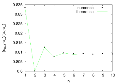
Figure 3: Plot of the ratio $\displaystyle\frac{c_{n+1}-c_{\infty}}{c_{n}-c_{\infty}}$ as a function of time step $n$. Numerical results were obtained by iterating rule 172 on a a configuration of length $10^{8}$ with periodic boundary conditions.

Using results of the previous section, eq. (11) can now be rewritten as

$$c_{n}=\frac{4^{n-1}+2^{n-1}F_{n+1}+2^{n-1}F_{n+2}}{2^{2n+1}},$$ (29)

which simplifies to

$$c_{n}=\frac{1}{8}+\frac{F_{n+3}}{2^{n+2}},$$ (30)

or, more explicitly, to

$$c_{n}=\frac{1}{8}+\frac{(1+\sqrt{5})^{n+3}-(1-\sqrt{5})^{n+3}}{2^{2n+5}\sqrt{5}}.$$ (31)

Obviously, $\lim_{n\rightarrow\infty}c_{n}=\frac{1}{8}$, in agreement with the numerical value reported in Wolfram (1994). We can see that $c_{n}$ converges toward $c_{\infty}$ exponentially fast, with some damped oscillations superimposed over the exponential decay. This is illustrated in Figure 3, where, in order to emphasize the aforementioned oscillations, instead of $c_{n}$ we plotted the ratio

$$d_{n}=\frac{c_{n+1}-c_{\infty}}{c_{n}-c_{\infty}}$$ (32)

as a function of $n$. One can show that $d_{n}$ converges to the half of ratio divina (golden ratio), $\psi/2\approx 0.809016\ldots$, as illustrated in Figure 3. We can see from this figure that the convergence is very fast and that the agreement between numerical simulations and the theoretical formula is nearly perfect.

8 Further results

Results obtained in the previous two sections suffice to compute block probabilities for all blocks of length up to 3. Proposition 6.1 together with eq. (8) yields formulas for $P_{n}(001)$, $P_{n}(101)$, and $P_{n}(111)$. Consistency conditions give $P_{n}(01)=P_{n}(001)+P_{n}(101)$. Furthermore $P_{n}(10)=P_{n}(01)$ due to the fact that $P_{n}(10)+P_{n}(00)=P_{n}(01)+P_{n}(00)=P_{n}(0)$. Applying consistency conditions again we have $P_{n}(1)=P_{n}(10)+P_{n}(11)$, hence $P_{n}(11)=P_{n}(1)-P_{n}(10)$, and, similarly, $P_{n}(00)=P_{n}(0)-P_{n}(10)$. This gives us probabilities of all blocks of length 2. Probabilities of blocks of length 3 can be obtained in a similar fashion:

$$P_{n}(000) =P_{n}(00)-P_{n}(100),$$

$$P_{n}(110) =P_{n}(11)-P_{n}(111),$$

$$P_{n}(011) =P_{n}(11)-P_{n}(111),$$

$$P_{n}(010) =P_{n}(01)-P_{n}(011).$$

The only missing probability, $P_{n}(100)$ is the same as $P_{n}(001)$ because $P_{n}(100)+P_{n}(000)=P_{n}(001)+P_{n}(000)=P_{n}(00)$. The following formulas summarize these results.

$$P_{n}(000) ={5}/{8}-{2}^{-n-2}F_{n+3}-{2}^{-n-4}F_{n+2},$$

$$P_{n}(001) ={1}/{8},$$

$$P_{n}(010) ={1}/{8}-{2}^{-n-3}F_{n+1},$$

$$P_{n}(011) ={2}^{-n-4}L_{n+2},$$

$$P_{n}(100) ={1}/{8},$$

$$P_{n}(101) ={2}^{-n-4}F_{n+2},$$

$$P_{n}(110) ={2}^{-n-4}L_{n+2},$$

$$P_{n}(111) ={2}^{-n-3}F_{n+3},$$

where $L_{n}=2F_{n+1}-F_{n}$ is the $n$-th Lucas number. We can also rewrite these formulas in terms of cardinalities of preimage sets using eq. (8), as stated below.

Theorem 8.1

Let ${\mathbf{f}}$ be the block evolution operator for CA rule 172. Then for any positive integer $n$ we have

$$\mathop{\mathrm{card}}{\mathbf{f}}^{-n}(000) = 5\cdot 4^{n}-2^{n+1}F_{n+3}-2^{n-1}F_{n+2},$$

$$\mathop{\mathrm{card}}{\mathbf{f}}^{-n}(001) = 4^{n},$$

$$\mathop{\mathrm{card}}{\mathbf{f}}^{-n}(010) = 4^{n}-2^{n}F_{n+1},$$

$$\mathop{\mathrm{card}}{\mathbf{f}}^{-n}(011) = 2^{n-1}L_{n+2},$$

$$\mathop{\mathrm{card}}{\mathbf{f}}^{-n}(100) = 4^{n},$$

$$\mathop{\mathrm{card}}{\mathbf{f}}^{-n}(101) = 2^{n-1}F_{n+2},$$

$$\mathop{\mathrm{card}}{\mathbf{f}}^{-n}(110) = 2^{n-1}L_{n+2},$$

$$\mathop{\mathrm{card}}{\mathbf{f}}^{-n}(111) = 2^{n}F_{n+3},$$

where $F_{n}$ is the $n$-th Fibonacci number, $\displaystyle F_{n}=\frac{\psi^{n}-(1-\psi)^{n}}{\sqrt{5}}$, $\psi=\frac{1}{2}+\frac{1}{2}\sqrt{5}$, and $L_{n}$ is the $n$-th Lucas number, $L_{n}=\psi^{n}+(1-\psi)^{n}$.

9 Concluding remarks

The method for computing block probabilities in cellular automata described in this paper is certainly not applicable to arbitrary CA rule. It will work only if the structure of level sets of preimage trees is sufficiently regular so that the level sets can be enumerated by some known combinatorial technique. Altough “chaotic” rules like rule 18, or complex rules such as rule 110 certainly do not belong to this category, in surprisingly many cases significant regularities can be detected in preimage trees. Usually, this applies to “simple” rules, those which in Wolfram classification belong to class I, class II, and sometimes class III. Rule 172 reported here is one of the most interesting among such rules, primarily because the density of ones does not converge exponentially to some fixed value as in many other cases, but exhibits subtle damped oscillations on top of the exponential decay. Furthermore, the appearance of Fibonacci and Lucas numbers in formulas for block probabilities is rather surprising.

One should add at this point that the convergence toward the steady state can be slower than exponential even in fairly “simple” cellular automata. Using similar method as in this paper, it has been found in Fukś and Haroutunian (2009) that in rule 14 the density of ones converges toward its limit value approximately as a power law. The exact formula for the density of ones in rule 14 involves Catalan numbers, and the structure of level sets is quite different than the one reported here. Rule 142 exhibits somewhat similar behavior too, as reported in Fukś (2006).

As a final remark, let us add that the results presented here assume initial measure $\mu_{1/2}$. This can be generalized to arbitrary $\mu_{p}$. In order to do this, one needs, instead of straightforward counting of preimages, to perform direct computation of their probabilities using methods based on Markov chain theory. Work on this problem is ongoing and will be reported elsewhere.

References

- Dynkin (1969) E. B. Dynkin. Markov Processes-Theorems and Problems. Plenum Press, New York, 1969.
- Ferrari et al. (2000) P. A. Ferrari, A. Maass, S. Martínez, and P. Ney. Cesàro mean distribution of group automata starting from measures with summable decay. Ergodic Theory Dynam. Systems, 20(6):1657–1670, 2000.
- Fukś (2006) H. Fukś. Dynamics of the cellular automaton rule 142. Complex Systems, 16:123–138, 2006.
- Fukś and Haroutunian (2009) H. Fukś and J. Haroutunian. Catalan numbers and power laws in cellular automaton rule 14. Journal of cellular automata, 4:99–110, 2009.
- Host et al. (2003) B. Host, A. Maass, and S. Martínez. Uniform Bernoulli measure in dynamics of permutative cellular automata with algebraic local rules. Discrete Contin. Dyn. Syst., 9(6):1423–1446, 2003.
- Lind (1984) D. A. Lind. Applications of ergodic theory and sofic systems to cellular automata. Phys. D, 10(1-2):36–44, 1984. Cellular automata (Los Alamos, N.M., 1983).
- Maass and Martínez (2003) A. Maass and S. Martínez. Evolution of probability measures by cellular automata on algebraic topological markov chains. Biol. Res., 36(1):113–118, 2003.
- Maass et al. (2006) A. Maass, S. Martínez, M. Pivato, and R. Yassawi. Asymptotic randomization of subgroup shifts by linear cellular automata. Ergodic Theory and Dynamical Systems, 26(04):1203–1224, 2006.
- Maass et al. (2006) A. Maass, S. Martínez, and M. Sobottka. Limit measures for affine cellular automata on topological markov subgroups. Nonlinearity, 19:2137–2147, Sept. 2006.
- Pivato and Yassawi (2002) M. Pivato and R. Yassawi. Limit measures for affine cellular automata. Ergodic Theory Dynam. Systems, 22(4):1269–1287, 2002.
- Pivato and Yassawi (2004) M. Pivato and R. Yassawi. Limit measures for affine cellular automata. II. Ergodic Theory Dynam. Systems, 24(6):1961–1980, 2004.
- Stanley (1986) R. P. Stanley. Enumerative combinatorics. Wadsworth and Brooks/Cole, Monterey, 1986.
- Wolfram (1994) S. Wolfram. Cellular Automata and Complexity: Collected Papers. Addison-Wesley, Reading, Mass., 1994.