Physical characteristics and non-keplerian orbital motion
of “propeller” moons embedded in Saturn’s rings

Abstract

We report the discovery of several large “propeller” moons in the outer part of Saturn’s A ring, objects large enough to be followed over the 5-year duration of the Cassini mission. These are the first objects ever discovered that can be tracked as individual moons, but do not orbit in empty space. We infer sizes up to 1–2 km for the unseen moonlets at the center of the propeller-shaped structures, though many structural and photometric properties of propeller structures remain unclear. Finally, we demonstrate that some propellers undergo sustained non-keplerian orbit motion.

1. Introduction

“Propeller” structures in a planetary ring, named for their characteristic two-armed shape, occur as the disturbance caused by a disk-embedded moon is carried downstream, which is forward (backward) on the side facing toward (away from) the planet per Kepler’s Third Law. Although no central moonlet has yet been directly resolved within a propeller, the observed structure allows us to infer both the locations and sizes of such moonlets. Predictions of such structures in Saturn’s rings (Spahn and Sremčević,, 2000; Sremčević et al.,, 2002; Seiß et al.,, 2005) led to their discovery in Cassini images (Tiscareno et al.,, 2006), followed by the realization that they reside primarily in a relatively narrow band in the mid-A ring (Sremčević et al.,, 2007). Further observations identified three “Propeller Belts” between 127,000 and 132,000 km from Saturn’s center, together containing 7000–8000 propeller moonlets with radius $R\gtrsim 0.15$ km, and exhibiting a steep power-law size distribution of $Q\sim 5$ (Tiscareno et al.,, 2008).

We report here that a population of propellers also exists in the outer part of the A ring, between the Encke Gap and the ring’s outer edge (i.e., between 133,700 and 136,700 km from Saturn’s center). These “trans-Encke” propellers are much less abundant but also much larger than those seen in the Propeller Belts (Fig. 1). Because of this, several trans-Encke propellers have been observed on multiple occasions with confidence that the same object is being viewed in each case, thus allowing conclusions to be drawn as to their persistence and orbital stability. No propellers are clearly apparent between the Propeller Belts and the Encke Gap.

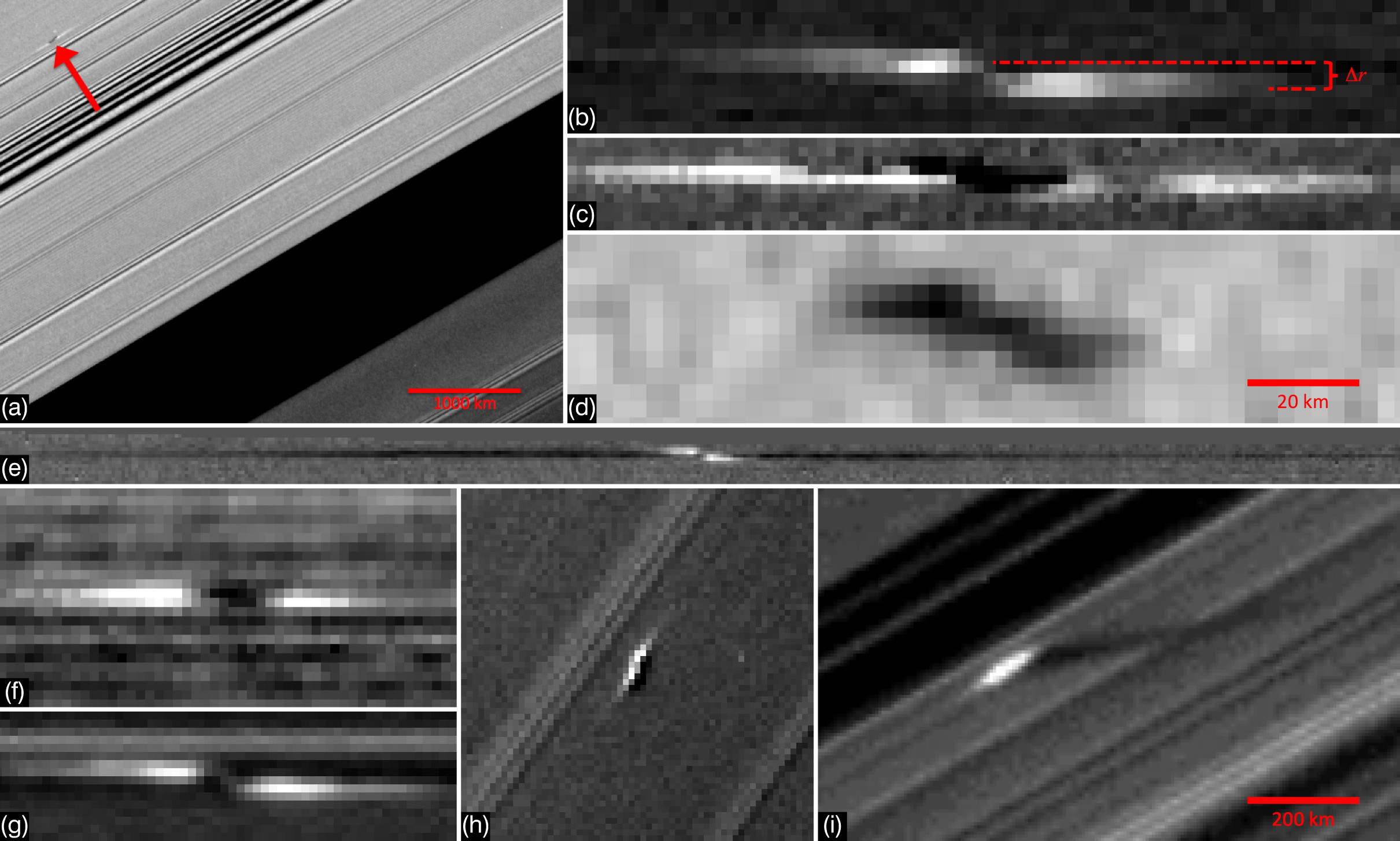
Figure 1.— Propellers as seen in selected Cassini images. Panel (a) shows a propeller in context of the Encke Gap and several density waves, while panels (h) and (i) show propellers casting shadows near the saturnian equinox (Section 2.2). The unseen moonlet is inferred to be at the center of the structure; its size is proportional to $\Delta r$ (Section 2.1), the radial offset between the two azimuthally-aligned lobes, as illustrated in panel (b). Panels (b), (c), and (d) show three views of the same propeller at the same scale, demonstrating how its appearance changes with viewing geometry. Non-equinox views are on the lit (b,e,g) or unlit (a,c,d,f) face of the rings. The scale bar in panel (d) also applies to panels (b), (c), (f), and (g). The scale bar in panel (i) also applies to panels (e) and (h). Image numbers, propeller nicknames, and apparition numbers are as follows: (a) N1597800527, “Santos-Dumont”, 081-081-A; (b) N1586641255, “Blériot”, 064-255-A; (c) N1597791119, “Blériot”, 081-054-A; (d) N1590907054, “Blériot”, 070-015-A; (e) N1544842586, “Blériot”, 035-299-A; (f) N1503243458, “Wright”, 013-020-A; (g) N1586628622, “Earhart”, 064-121-A; (h) N1620657077, “Blériot”, 110-088-A; and (i) N1628846480, “Earhart”, 116-008-A.

Each propeller observation is given an alphanumeric identifier, following the convention of Tiscareno et al., (2008). However, propellers that are seen in multiple widely-separated apparitions are given nicknames that can serve to tie together the various observations. To confirm the identity of objects in widely-separated apparitions, we check not only that the radial locations are the same but also that the longitudes are consistent (with residuals as specified in Section 3) with keplerian motion at that orbital radius.

2. Size and photometry

2.1. Size from radial offset

The size of the central moonlet, which is not directly seen, can be inferred from the radial offset $\Delta r$ between the leading and trailing azimuthally-aligned lobes of the propeller (Fig. 1b). Initial simulations suggested that the radial separation between the density-depleted regions on either side of a moonlet is $\Delta r\sim 4r_{H}$ (Seiß et al.,, 2005), where $r_{H}$ is the Hill radius; interpretation of recent $N$-body simulations including mutual self-gravity and particle-size distributions is more complex due to moonlet accretion during the simulation, but the relationship $\Delta r\sim 4r_{H}$ appears to hold (Lewis and Stewart,, 2009). Assuming that the density of the central moonlet is such that it fills its Roche lobe, and thus the moonlet’s mean radius $\bar{R}$ is approximately 0.72 times its Hill radius (Porco et al.,, 2007), we then expect $\bar{R}\sim 0.18\Delta r$.

In the Propeller Belts, what appear morphologically to be the density-depleted regions within individual propellers unexpectedly appear bright against the background ring. Sremčević et al., (2007) suggested brightening due to temporary liberation of regolith, while Tiscareno et al., (2010) investigated the role that disruption of self-gravity wakes might play in brightening propeller structures. Whatever the cause, brightened regions may blend, or even be primarily associated, with density-enhanced regions at larger values of $\Delta r$ (e.g., Sremčević et al., (2007) suggested $\Delta r\sim(9\pm 1)r_{H}$ for density enhancements), so that $\bar{R}\lesssim 0.18\Delta r$ should be regarded as an upper limit.

Some of the largest propellers seen in the trans-Encke region show, for the first time, both bright and dark components (Figs. 1b through 1d). For these, the density-enhanced and density-depleted regions can be clearly separated, under the assumption that the density-enhanced regions are brighter (darker) on the lit (unlit) face of the rings. Indeed, in some images of giant propellers the morphology is clearly that of density-enhanced regions, including the bright ribbon connecting “Earhart’s” two bright lobes (Fig. 1g) and “Blériot’s” bright lobes that are sometimes seen wrapped around dark wings (density-depleted regions) with a great deal more azimuthal extent (Fig. 1e).

However, our measurements of $\Delta r$ in these cases (Fig. 2) show that further photometric and theoretical understanding is needed before the size of the central moonlet can be confidently obtained from $\Delta r$ to accuracy better than a factor of several (making the mass uncertain by about an order of magnitude). We expected to find that relative-bright features on the lit face of the rings and relative-dark features on the unlit face would be the same (density-enhanced) components of the propeller, and similarly that relative-dark features on the lit face and relative-bright features on the unlit face would be the same (density-depleted) components, but in measured $\Delta r$ values for propeller “Blériot” (the only one for which all four aspects are seen) the radial separations all differ from each other. Similarly, while relative-bright features on the lit face do have consistently larger values of $\Delta r$ than relative-bright features on the unlit face, as expected for (respectively) density-enhanced and density-depleted components, the ratios between the two are not consistent among the four propellers (“Blériot”, “Post”, “Santos-Dumont”, and “Wright”) that have been observed on both the lit and unlit faces of the rings.

Figure 2.— Observed radial offsets $\Delta r$ for all propellers with measurement errors $<0.7$ km. Error bars (1-sigma) are given, but in many cases are smaller than the plotted symbol. The right-hand axis gives the inferred radius of the central moonlet assuming internal density equal to the Roche critical density and $\Delta r\sim 4r_{H}$; we emphasize that the latter assumption cannot be valid for all cases listed here (see Section 2.1). From shadow lengths we directly measure the vertical height of the propeller, which should be comparable to the moonlet radius (Section 2.2). For “Blériot”, the only propeller with observed relative-dark components on the lit face of the rings or with observed relative-bright components on the unlit face of the rings, the radial offsets for lit-dark and unlit-bright do not agree, nor do unlit-dark and lit-bright, as might have been expected. Furthermore, the four propellers observed on both the lit and unlit faces of the rings do not have a consistent ratio of lit-bright to unlit-bright.

The unexpected complexity of these observations indicates that the photometry of propellers is highly dependent on viewing geometry, perhaps including solar incidence angle and viewer’s emission angle in addition to the more commonly-considered phase angle, and may also simply vary with time. Such photometric variations may be due to the poorly-understood details of propeller structure and/or to differing particle-size properties between propeller and background.

2.2. Size from shadows

A saturnian equinox, which occurs every 14.7 yr, took place in 2009 August. During this event, the Sun shone nearly edge-on to the ring plane, causing any vertical structure to cast long shadows. Several propellers were observed during this period, along with their shadows (Figs. 1h and 1i). The azimuthally-distributed morphology of the shadows indicates that they were cast by the propeller structures as a whole, and not directly by the central moonlets. However, the vertical extent of a propeller structure should be comparable to the size of its moonlet, as it is the moonlet’s gravity that pulls material out of the ring plane (preliminary results from simulations corroborate this notion; M. C. Lewis, pers. comm.). Shadow lengths indicate that “Blériot’s” propeller has a vertical height of $0.43\pm 0.03$ km above the ring, while other propellers have shadow-inferred vertical heights of 0.12 km (“Santos-Dumont”), 0.16 km (116-006-A) and 0.26 km (“Earhart”). The main body of the A ring has a vertical thickness on the order of a $\mathrm{few}\times 0.01$ km (Tiscareno et al.,, 2007; Hedman et al.,, 2007; Colwell et al.,, 2009).

2.3. Size distribution

Figure 3.— Particle size distribution for Saturn’s A Ring. The solid line and open square denote the Voyager RSS size distribution for the ring continuum, converted to integral format from the solution for 2.14 $R_{\mathrm{S}}=1$29,100 km given in Table III of Zebker et al., (1985). The open diamond is obtained from two known moons (Pan and Daphnis) of radius $\gtrsim 4$ km in the entire A Ring. The open circles denote values for the Propeller Belts, from Tiscareno et al., (2006, 2008). The filled circle shows a result from this work for the trans-Encke region. The error bars reflect the systematic error due to model-dependency in the conversion from $\Delta r$ to moonlet size (the left-hand side of the error bar corresponds to $\Delta r\sim 4r_{H}$, while the right-hand side of the error bar corresponds to $\Delta r\sim 8r_{H}$, see Section 2.1); it is important to note that data points will slide along the error bars in concert, preserving their relative positions and thus the inferred power law. The change in linestyle from dashed to dotted is to indicate that the open circles and the filled circles represent data from different regions within the A Ring, so that there is no reason to assume that they must fall on the same size-distribution curve, and furthermore that large propellers appear to be absent in the Propeller Belts while small propellers are absent in the trans-Encke region (Section 2.3).

The propeller-belt and the giant-propeller populations may in fact have very similar size-distribution curves. The complete azimuthal scan from Orbit 35 found 19 propellers between 133,700 and 135,000 km with $\Delta r\gtrsim 2$ km, and the partial azimuthal scan (65%-complete) from Orbit 64 found 16, both of which give a surface density of $2\times 10^{-8}$ km^-2. As shown in Fig. 3, this is the same number that one gets by extrapolating from the Propeller Belts’ surface density and power law $Q\sim 5$ (Tiscareno et al.,, 2008).

Figure 4.— Observed longitude of the propeller “Blériot” over 4 years, with a linear trend (616.7819329^∘/day) subtracted off. Only data points with measurement errors $\sigma<0.01^{\circ}$ are shown. Error bars (1-sigma) are given, but in many cases are smaller than the plotting symbol. Panel (a) shows all the data, while panels (b), (c), and (d) contain subsets of the data shown in greater detail. The residuals to the linear trend (horizontal dotted line) are less than $\pm 300$ km, but are clearly not randomly distributed. The dotted line indicates a linear-plus-sinusoidal fit to all the data, with an amplitude of $0.11^{\circ}$ and a period of 3.68 yr. The solid lines indicate piecewise quadratic fits, corresponding to a constant drift in semimajor axis; in particular, the data from mid-2006 to early-2007 (panel c) are fit by a linear trend with a constant acceleration of -0.0096^′′/day² ($\dot{a}=+0.11$ km/yr), while the data from late-2007 to early-2009 (panel d) are fit by a linear trend with a constant acceleration of +0.0023^′′/day² ($\dot{a}=-0.04$ km/yr).

Table 1Orbit fits for trans-Encke propellers

					Longitude			Rms deviation
Nickname	$n$, ∘/daya		$a$, kma		at epochb	# imagesc	Time interval	in km	in longitude
Earhart	624.	529897(2)	133797.	8401(3)	57.85∘	3	2006–2009 (2.7 yr)	730	0.31∘
Post	624.	4867(3)	133803.	99(4)	58.09∘	3	2006–2008 (1.7 yr)	12	0.01∘
Sikorsky	623.	917736(1)	133885.	0475(2)	70.37∘	3	2005–2008 (3.1 yr)	230	0.10∘
Curtiss	623.	7473	133909.	36	210.04∘	2	2006–2008 (1.7 yr)
Lindbergh	623.	3176(2)	133970.	69(2)	112.08∘	3	2005–2008 (3.0 yr)	71	0.03∘
Wright	622.	5527	134080.	03	251.85∘	2	2005–2006 (1.3 yr)
Kingsford Smith	620.	761649(2)	134336.	9350(3)	202.44∘	4	2005–2008 (2.9 yr)	670	0.28∘
Hinkler	619.	80519(1)	134474.	639(2)	58.85∘	3	2006–2008 (1.3 yr)	360	0.15∘
Santos-Dumont	619.	458729(1)	134524.	6067(2)	324.11∘	9	2005–2009 (4.3 yr)	670	0.28∘
Richthofen	617.	7011	134778.	83	122.90∘	2	2006–2007 (0.3 yr)
Blériot	616.	7819329(6)	134912.	24521(8)	193.65∘	89	2005–2009 (4.2 yr)	210	0.09∘
a Formal error estimates, shown in parentheses for the last digit, are for the best-fit linear trend in longitude. They are
much smaller than the rms deviations in longitude, given in the right-hand column.
b Epoch is 2007 January 1 at 12:00:00 UTC (JD 1782806.0). All orbit fits assume $e=0$ and $i=0$.
c Not including images of insufficient quality to include in the orbit fit.

However, if the two populations do have the same size-distribution slope and intercept, they are likely truncated so that they do not actually overlap. The same radial scans that discovered the Propeller Belts (Tiscareno et al.,, 2008) clearly showed no small propellers elsewhere in the A ring, including the trans-Encke region, so it would appear that only giant propellers occur in the latter. On the other hand, while fewer high-resolution (better than 3 km/px) images have been taken of the Propeller Belts, compared with the trans-Encke region, the ratio is only a factor of several, which makes it likely (but not conclusively proven) that giant propellers are missing in the Propeller Belts. Even the largest propellers observed in the Propeller Belts have $\Delta r<1.3$ km (Tiscareno et al.,, 2008), while nearly all observed trans-Encke propellers have $\Delta r$ larger than this value (Fig. 2).

3. The orbital evolution of “Blériot”

At least 11 propellers have been seen at multiple widely-separated instances, but “Blériot” is of particular interest as the largest and most frequently detected (Figs. 1b, 1c, 1d, 1e, and 1h). It has appeared in more than one hundred separate Cassini ISS images spanning a period of four years, and was serendipitously detected once in a stellar occultation observed by the Cassini UVIS instrument (Colwell et al.,, 2008).

Analysis of the orbit of “Blériot” confirms that it is both long-lived and reasonably well-characterized by a keplerian path. As Fig. 4 shows, a linear fit to the longitude with time (corresponding to a circular orbit) results in residuals of $\pm 300$ km (0.13^∘ longitude). However, those residuals are some 50 times greater than the mean measurement errors; furthermore, the residuals are far from randomly distributed, with a strong indication of coherent motions superposed atop the linear trend. Analysis of the orbits of other propellers, though less well-sampled in time, similarly shows variations in longitude of up to 1000 km (Table 1), easily small enough to confirm that a single object is being observed but much larger than the measurement errors.

After a linear trend, the next-simplest functional form available is a quadratic, which corresponds to a constant angular acceleration, or (equivalently) a linear drift of the semimajor axis with time. A global quadratic fit to all data points does hardly better than the global linear fit and is not shown in Fig. 4.

Two possible functional forms for the non-keplerian motion are 1) a linear trend plus a sinusoidal variation of the longitude with time, which is shown by the dotted line in Fig. 4, and 2) a piecewise fit carried out by grouping the data into four segments and fitting each segment to a linear or quadratic trend, shown by the solid lines in Fig. 4. The most likely physical mechanism for the former is some kind of resonant interaction, perhaps with one of the many larger moons in or near the rings, although no resonance has yet been identified that might plausibly explain “Blériot’s” motions. The most likely physical mechanism for the latter is that “Blériot” periodically suffers collisions (Lewis and Stewart,, 2009) that jostle its orbit onto a new one, but that in between such kicks its semimajor axis drifts linearly due to gravitational and/or collisional interactions with the disk.

Continued investigation of the non-keplerian motion of propeller moons is ongoing.

Table S1Observing information for images used in this paper.

		# of		Incidence	Emission	Phase	Radial	Azimuthal
Orbit	Image Identifier	Images	Date	Angleb	Angleb	Angle	Resolutionc	Resolutionc
007	N1493569190	1	2005-120	111.9∘	109.6∘	40.2∘	8.6	25.1
007	N1493619126 – 42136	20	2005-121	111.8∘	111.0∘	33.6∘	6.9	18 – 20
007	N1493715564 – 24205	3	2005-122	111.8∘	115.2∘	12.2∘	3 – 5	3 – 6
008	N1495108987 – 35027	17	2005-138	111.7∘	109.6∘	41.7∘	8.9	25 – 28
009	N1496871927 – 2034	3	2005-158	111.5∘	109.4∘	18.5∘	3.8	6.6
012	N1501228513 – 9785	4	2005-209	110.9∘	107.4∘	55.7∘	13.8	19 – 24
013	N1503243458	1	2005-232	110.7∘	52.1∘	162.3∘	1.3	1.1
028	N1537022412	1	2006-258	105.9∘	75.0∘	175.8∘	13.0	49.6
029	N1538205758	1	2006-271	105.7∘	58.7∘	161.0∘	10.1	19.5
030	N1539660972 – 8180	2	2006-289	105.4∘	49.0∘	151.2∘	10.6	16.1
031	N1540581552	1	2006-299	105.3∘	106.6∘	117.8∘	5.9	10.7
033	N1542569654 – 70226	2	2006-322	105.0∘	91.9∘	147.9∘	7.2	150 – 174
033	N1543202188 – 695	2	2006-329	104.9∘	59.8∘	160.5∘	10.2	20.4
034	N1543354660 – 5569	2	2006-331	104.9∘	69.6∘	159.0∘	10.2	29.2
035	N1544813989 – 43793	20	2006-348/349	104.6∘	117∘ – 150∘	27∘ – 64∘	2.7	2 – 5
036	N1545570886 – 1332	2	2006-357	104.5∘	54.9∘	159.2∘	11.8	20.6
036	N1546726425 – 798	2	2007-005	104.3∘	35.3∘	133.6∘	10.4	12.8
037	N1548113882 – 946	2	2007-021	104.1∘	34.0∘	110.2∘	10.7	10.4
039	N1551257093 – 309107	2	2007-058	103.6∘	34.8∘	104.9∘	10.2	12.4
041	N1552822117 – 477	2	2007-076	103.3∘	35.5∘	108.8∘	10.6	13.1
041	N1554027273 – 8323	4	2007-090	103.1∘	51.8∘	82.2∘	11.9	19.2
042	N1554731052	1	2007-098	103.0∘	118.9∘	128.2∘	2.7	5.6
043	N1556183373 – 202155	6	2007-115	102.8∘	123∘ – 138∘	21∘ – 43∘	3.1 – 4.2	2.6 – 4.5
045	N1558418169	1	2007-141	102.4∘	71.0∘	72.4∘	13.7	23.7
045	N1559371611 – 77	3	2007-152	102.2∘	83.4∘	51.5∘	12.5	105.4
053	N1575154715 – 65751	9	2007-334/335	99.5∘	80.4∘	52.2∘	8.7	49 – 52
054	N1577141652 – 95	2	2007-356	99.2∘	75.9∘	23.9∘	11.9	33.7
055	N1577829421 – 30077	3	2007-365	99.0∘	57.3∘	64.8∘	9.6	17.7
055	N1578422585 – 9943	12	2008-007	98.9∘	78.1∘	21.8∘	9.9	47.6 – 49.0
056	N1579166576	1	2008-016	98.8∘	123.8∘	66.2∘	2.5	4.5
057	N1579792597 – 3315	3	2008-023	98.7∘	62.7∘	42.7∘	10.2	22.2
061	N1584357723 – 73623	2	2008-067	97.9∘	77.8∘	20.9∘	12.4	14.7
064	N1586618575 – 41255	17	2008-102	97.5∘	141∘ – 175∘	49∘ – 103∘	1.7 – 2.8	1.8 – 3.4
065	N1587553446 – 4566	5	2008-113	97.3∘	104.5∘	14.5∘	5.5	21.8
068	N1589849522	1	2008-139	96.9∘	112.5∘	37.3∘	5.3	8.4
070	N1590907054 – 8480	2	2008-152	96.7∘	56.6∘	42.5∘	6.3	7 – 11
070	N1591067764 – 85510	5	2008-154	96.7∘	140∘ – 154∘	71∘ – 82∘	2.3	2.1
071	N1591525824	1	2008-159	96.6∘	58.8∘	37.9∘	6.3	11.1
080	N1597462656	1	2008-228	95.6∘	87.1∘	26.5∘	7.4	58.4
080	N1597487541 – 8439	4	2008-228	95.6∘	83.4∘	16.7∘	7.7	20 – 60
081	N1597775567 – 800527	4	2008-231/232	95.5∘	25∘ – 45∘	94∘ – 105∘	3.0	2.7
090	N1603444112	1	2008-297	94.5∘	37.0∘	58.9∘	4.4	5.5
092	N1604569991 – 70034	2	2008-310	94.3∘	69.3∘	32.7∘	8.0	12.7
098	N1608800086 – 341	3	2008-359	93.5∘	24.8∘	69.9∘	5.3	4.9
102	N1612496648	1	2009-036	92.9∘	128.6∘	59.0∘	9.5	7.0
105	N1614861737	1	2009-063	92.5∘	66.5∘	34.5∘	7.1	17.8
110	N1620656882 – 7077	2	2009-130	91.4∘	117.5∘	59.9∘	5.6	12.2
114	N1626159520	1	2009-194	90.4∘	41.8∘	77.3∘	9.7	7.2
114	N1626320702	1	2009-196	90.4∘	49.7∘	89.4∘	11.5	13.1
115	N1627613635	1	2009-211	90.2∘	61.2∘	99.1∘	10.1	20.8
116	N1628845563 – 6513	7	2009-225	90.0∘	72.0∘	82∘ – 92∘	8 – 11	9 – 13
a For lines referring to multiple images, variation in each parameter is in the last significant figure.
b Measured from the direction of Saturn’s north pole (ring-plane normal), so that angles $>90^{\circ}$ denote the southern
hemisphere.
c In km/pixel.

Table S2Fitted sizes for multiply-observed trans-Encke propellers.

Namea,b	Lit/Unlit	B/Dc	$\Delta r$, km		Inferred $\bar{R}$, kmd	# images	Reduced $\chi^{2}$
064-103-A	Lit	B	2.16$\pm$	0.12	$0.37\pm 0.02$	2	13.73
Blériot	Lit	B	5.50$\pm$	0.05	$0.95\pm 0.01$	6	9.99
Blériot	Lit	D	1.78$\pm$	0.07	$0.31\pm 0.01$	7	3.75
Blériot	Unlit	B	4.15$\pm$	0.18	$0.72\pm 0.03$	6	2.24
Blériot	Unlit	D	6.60$\pm$	0.27	$1.14\pm 0.05$	3	0.58
Curtiss	Lit	B	3.11$\pm$	0.10	$0.54\pm 0.02$	1
Earhart	Lit	B	5.17$\pm$	0.11	$0.90\pm 0.02$	2	19.58
Hinkler	Lit	B	1.85$\pm$	0.24	$0.32\pm 0.04$	2	0.00
Kingsford Smith	Lit	B	5.32$\pm$	0.10	$0.92\pm 0.02$	2	0.04
Lindbergh	Lit	B	1.33$\pm$	0.12	$0.23\pm 0.02$	2	0.15
Post	Lit	B	3.34$\pm$	0.07	$0.58\pm 0.01$	3	24.63
Post	Unlit	B	2.97$\pm$	0.43	$0.51\pm 0.07$	1
Richthofen	Lit	B	2.44$\pm$	0.16	$0.42\pm 0.03$	2	0.78
Santos-Dumont	Lit	B	4.34$\pm$	0.22	$0.75\pm 0.04$	3	22.27
Santos-Dumont	Unlit	B	2.92$\pm$	0.32	$0.51\pm 0.06$	1
Sikorsky	Lit	B	2.56$\pm$	0.21	$0.44\pm 0.04$	2	0.39
Wright	Lit	B	2.94$\pm$	0.41	$0.51\pm 0.07$	1
Wright	Unlit	B	0.72$\pm$	0.11	$0.12\pm 0.02$	1
Wright	Unlit	D	0.73$\pm$	0.28	$0.13\pm 0.05$	1
a Alphanumeric identifier for a single apparition (see Table S4), or nickname used to tie
together multiple apparitions of the same object.
b Propellers seen only once are not listed here, as their measured $\Delta r$ values are already given
in Table S4 and Fig. 2.
c Relative-bright (B) or relative-dark (D), with respect to image background.
d Mean radius of moonlet assuming internal density equal to the Roche critical density and
$\Delta r\sim 4r_{H}$; we emphasize that the latter assumption cannot be valid for all cases listed here
(see text).

Table S3Vertical heights of propellers, inferred from near-equinox shadows.

		Solar	Shadow		Inferred
		Incidence	Length,		Obstacle
Namea	Image	Angleb (∘)	km		Height, km	Nicknamea
110-087-A	N1620656882	91.42	19$\pm$	7	$0.47\pm 0.17$	Bleriot
110-088-A	N1620657077	91.42	20$\pm$	7	$0.49\pm 0.17$	Bleriot
114-001-A	N1626159520	90.44	55$\pm$	7	$0.424\pm 0.057$	Bleriot
114-015-A	N1626320702	90.41	49$\pm$	13	$0.353\pm 0.092$	Bleriot
116-004-A	N1628845780	89.96	221$\pm$	10	$0.136\pm 0.006$	Santos-Dumont
116-005-A	N1628845813	89.96	184$\pm$	10	$0.113\pm 0.006$	Santos-Dumont
116-006-A	N1628846210	89.96	257$\pm$	10	$0.159\pm 0.006$	116-006-A
116-007-A	N1628846243	89.96	252$\pm$	10	$0.156\pm 0.006$	116-006-A
116-008-A	N1628846480	89.96	426$\pm$	9	$0.263\pm 0.006$	Earhart
116-009-A	N1628846513	89.96	419$\pm$	9	$0.259\pm 0.006$	Earhart
a As in Table S2.
b Measured from Saturn’s north pole.

Table S4Fitted sizes for trans-Encke propellers.

Namea	Image	B/Db	[ line, sample ]	$\Delta\ell$ (km)c		$\Delta r$ (km)		Match/Nicknamed
007-030-A	N1493619126	B	[ 217.2,1017.1 ]	51.2$\pm$	2.8	6.5$\pm$	0.9	Blériot
007-031-A	N1493619321	B	[ 247.4, 857.4 ]	53.4$\pm$	2.7	8.4$\pm$	0.7	Blériot
007-031-A	”	D	”			0.817$\pm$	0.868	Blériot
007-032-A	N1493619516	B	[ 269.3, 701.2 ]	48.8$\pm$	3.7	7.4$\pm$	1.0	Blériot
007-032-A	”	D	”			1.488$\pm$	0.696	Blériot
007-033-A	N1493619711	B	[ 278.2, 540.6 ]	54.3$\pm$	2.9	7.7$\pm$	0.9	Blériot
007-033-A	”	D	”			1.988$\pm$	0.658	Blériot
007-034-A	N1493619906	B	[ 277.9, 386.3 ]	45.9$\pm$	3.9	5.6$\pm$	1.8	Blériot
007-034-A	”	D	”			0.976$\pm$	0.660	Blériot
007-035-A	N1493620101	B	[ 267.1, 227.0 ]	48.4$\pm$	7.6	5.9$\pm$	2.0	Blériot
007-035-A	”	D	”			1.419$\pm$	0.497	Blériot
007-036-A	N1493620296	B	[ 244.9, 68.8 ]	47.2$\pm$	4.2	4.8$\pm$	1.2	Blériot
007-036-A	”	D	”			1.695$\pm$	0.670	Blériot
007-087-A	N1493715564	D	[ 318.8, 475.4 ]			2.253$\pm$	0.125	Blériot
007-173-A	N1493721598	B	[ 324.5, 924.0 ]	33.1$\pm$	1.5	1.9$\pm$	0.8
007-199-A	N1493724205	B	[ 121.4, 670.5 ]	31.0$\pm$	0.8	0.7$\pm$	0.5
008-159-A	N1495131307	B	[ 678.8, 814.2 ]	40.9$\pm$	8.5	6.1$\pm$	3.4	Blériot
008-160-A	N1495131555	B	[ 701.8, 659.8 ]	46.8$\pm$	5.9	5.4$\pm$	1.9	Blériot
008-161-A	N1495131803	B	[ 709.3, 502.0 ]	53.8$\pm$	5.0	3.9$\pm$	1.5	Blériot
008-162-A	N1495132051	B	[ 703.7, 350.0 ]	50.4$\pm$	5.9	5.8$\pm$	2.0	Blériot
008-163-A	N1495132299	B	[ 683.4, 193.8 ]	50.1$\pm$	6.5	6.3$\pm$	2.5	Blériot
008-164-A	N1495132547	B	[ 649.2, 33.3 ]	67.7$\pm$	5.1	1.7$\pm$	1.7	Blériot
009-023-A	N1496871927	B	[ 760.7, 590.4 ]	31.0$\pm$	1.9	7.7$\pm$	0.7	Santos-Dumont
009-025-A	N1496872000	B	[ 763.8, 585.6 ]	28.3$\pm$	2.2	6.2$\pm$	0.6	Santos-Dumont
009-026-A	N1496872034	B	[ 763.2, 584.6 ]	20.4$\pm$	2.7	8.1$\pm$	0.9	Santos-Dumont
012-049-A	N1501228513	B	[ 977.0, 122.7 ]	68.9$\pm$	5.1	15.7$\pm$	1.9	Blériot
012-050-A	N1501228937	B	[ 908.7, 90.2 ]	48.1$\pm$	9.4	14.0$\pm$	2.8	Blériot
012-051-A	N1501229361	B	[ 834.0, 61.3 ]	63.7$\pm$	5.4	14.0$\pm$	2.1	Blériot
012-052-A	N1501229785	B	[ 756.7, 28.8 ]	61.6$\pm$	6.7	14.6$\pm$	2.0	Blériot
013-020-A	N1503243458	D	[ 221.3, 425.3 ]	3.4$\pm$	0.5	0.7$\pm$	0.3	Wright
013-020-A	”	B	[ 221.6, 426.0 ]	22.1$\pm$	0.4	0.7$\pm$	0.1	Wright
031-017-A	N1540581552	B	[ 417.0, 57.1 ]	54.9$\pm$	2.0	8.7$\pm$	0.6	Blériot
033-070-A	N1543202188	B	[ 617.2, 77.6 ]	97.6$\pm$	5.8	8.5$\pm$	1.8	Blériot
033-071-A	N1543202695	B	[ 199.5, 51.4 ]	130.1$\pm$	9.5	1.1$\pm$	2.4	Blériot
034-009-A	N1543354660	B	[ 566.8, 673.0 ]	119.4$\pm$	6.4	9.6$\pm$	2.8	Blériot
034-010-A	N1543355569	B	[ 44.0, 594.4 ]	126.6$\pm$	9.7	2.3$\pm$	2.0	Blériot
035-028-A	N1544813989	B	[ 790.8, 322.6 ]	33.6$\pm$	0.4	5.3$\pm$	0.1	Kingsford Smith
035-067-A	N1544818130	B	[ 966.8, 787.1 ]	13.9$\pm$	0.4	2.5$\pm$	0.2	Richthofen
035-076-A	N1544819124	B	[ 580.3, 27.9 ]	14.7$\pm$	1.4	4.2$\pm$	0.4
035-094-A	N1544820869	B	[ 629.5, 842.8 ]	17.7$\pm$	0.2	3.1$\pm$	0.1	Curtiss
035-130-A	N1544824600	B	[ 919.6, 137.0 ]	11.6$\pm$	0.8	2.7$\pm$	0.7
035-153-A	N1544826831	B	[ 651.7, 604.0 ]	12.6$\pm$	0.6	1.4$\pm$	0.3	Lindbergh
035-153-B	”	B	[ 942.4, 687.6 ]	9.0$\pm$	0.3	3.1$\pm$	0.2
035-164-A	N1544828015	B	[ 646.5, 487.7 ]	13.3$\pm$	0.3	2.0$\pm$	0.2
035-189-A	N1544830440	B	[ 635.6, 298.9 ]	20.6$\pm$	0.4	2.1$\pm$	0.2
035-193-A	N1544830828	B	[ 805.7, 282.4 ]	14.0$\pm$	0.4	2.6$\pm$	0.3
035-206-A	N1544832207	B	[ 827.9, 83.0 ]	10.8$\pm$	0.5	1.9$\pm$	0.4	Hinkler
035-209-A	N1544832498	B	[ 608.8, 998.8 ]	16.0$\pm$	0.8	2.2$\pm$	0.6	Sikorsky
035-210-A	N1544832595	B	[ 617.1, 85.1 ]	16.3$\pm$	0.3	2.6$\pm$	0.2	Sikorsky
035-242-A	N1544835939	B	[ 836.7, 63.2 ]	29.3$\pm$	0.6	3.5$\pm$	0.3	Santos-Dumont
035-260-A	N1544837802	B	[ 699.5, 477.1 ]	14.3$\pm$	0.8	2.9$\pm$	0.4	Wright
035-296-A	N1544842159	B	[ 595.8, 129.0 ]	26.0$\pm$	1.6	3.5$\pm$	0.4
035-299-A	N1544842586	B	[ 1019.4, 405.8 ]	50.6$\pm$	1.3	5.4$\pm$	0.2	Blériot
035-299-A	N1544842586	D	”			1.555$\pm$	0.092	Blériot
035-306-A	N1544843697	B	[ 612.5, 943.8 ]	40.2$\pm$	1.3	4.3$\pm$	0.3	Post
035-307-A	N1544843793	B	[ 601.4, 32.0 ]	38.8$\pm$	1.3	4.6$\pm$	0.2	Post
035-307-B	”	B	[ 601.7, 161.1 ]	43.9$\pm$	1.2	6.0$\pm$	0.2	Earhart
036-070-A	N1546726798	B	[ 235.7, 3.7 ]	88.8$\pm$	2.0	3.7$\pm$	0.6	Blériot
037-001-A	N1548113882	B	[ 136.2, 732.2 ]	145.7$\pm$	5.2	4.9$\pm$	1.0	Blériot
037-002-A	N1548113946	B	[ 210.0, 665.4 ]	122.9$\pm$	5.0	7.0$\pm$	0.9	Blériot
039-009-A	N1551257093	B	[ 260.0,1001.1 ]	112.2$\pm$	3.7	5.0$\pm$	1.0	Blériot
039-140-A	N1551309107	B	[ 377.1, 994.7 ]	104.9$\pm$	3.2	5.7$\pm$	0.9	Blériot
041-088-A	N1552822117	B	[ 108.5, 912.0 ]	112.0$\pm$	5.8	3.1$\pm$	1.8	Blériot
041-089-A	N1552822477	B	[ 551.2, 998.7 ]	123.2$\pm$	4.0	4.1$\pm$	1.3	Blériot
042-045-A	N1554731052	B	[ 264.7, 484.6 ]	16.3$\pm$	1.8	2.1$\pm$	0.4	Richthofen
Continued on next page

Table S4Fitted sizes for trans-Encke propellers (continued from previous page)

Namea	Image	B/Db	[ line, sample ]	$\Delta\ell$ (km)c		$\Delta r$ (km)		Match/Nicknamed
043-053-A	N1556183373	B	[ 74.7, 980.3 ]	16.3$\pm$	1.7	0.7$\pm$	0.9	043-054-A
043-054-A	N1556183485	B	[ 80.4, 63.1 ]	17.3$\pm$	0.5	1.7$\pm$	0.4	043-053-A
043-069-A	N1556185283	B	[ 390.0, 559.6 ]	31.3$\pm$	0.8	3.3$\pm$	0.2
043-083-A	N1556186850	B	[ 343.4, 860.1 ]	11.3$\pm$	0.4	1.1$\pm$	0.5
043-162-A	N1556196060	B	[ 64.8, 456.3 ]	42.0$\pm$	1.1	5.3$\pm$	0.3	Blériot
043-212-A	N1556202155	B	[ 333.1, 253.5 ]	20.1$\pm$	0.5	0.6$\pm$	0.4
064-007-A	N1586618575	B	[ 999.3, 689.4 ]	3.6$\pm$	0.2	2.0$\pm$	0.5
064-073-A	N1586624372	B	[ 332.5, 451.0 ]	11.0$\pm$	0.6	1.3$\pm$	0.4
064-076-A	N1586624630	B	[ 330.4, 226.4 ]	9.4$\pm$	0.3	2.5$\pm$	0.2
064-092-A	N1586626006	B	[ 315.0, 655.2 ]	9.5$\pm$	0.3	2.5$\pm$	0.2
064-103-A	N1586627074	B	[ 35.6, 85.0 ]	10.4$\pm$	0.2	2.0$\pm$	0.1	064-104-A
064-104-A	N1586627160	B	[ 72.0, 988.3 ]	10.8$\pm$	0.4	3.4$\pm$	0.3	064-103-A
064-109-A	N1586627590	B	[ 21.8, 138.8 ]	11.6$\pm$	0.9	1.8$\pm$	0.3	Hinkler
064-114-A	N1586628020	B	[ 19.8, 675.4 ]	9.7$\pm$	0.3	2.3$\pm$	0.2
064-121-A	N1586628622	B	[ 382.4, 550.5 ]	37.6$\pm$	0.8	4.9$\pm$	0.1	Earhart
064-133-A	N1586629654	B	[ 323.8, 501.9 ]	18.6$\pm$	1.0	2.5$\pm$	0.2
064-146-A	N1586630893	B	[ 374.2, 264.5 ]	19.4$\pm$	0.2	3.1$\pm$	0.1	Post
064-163-A	N1586632355	B	[ 332.5, 182.9 ]	11.5$\pm$	0.6	3.4$\pm$	0.2
064-176-A	N1586633595	B	[ 304.5, 464.1 ]	15.0$\pm$	0.3	1.3$\pm$	0.1	Lindbergh
064-208-A	N1586636591	B	[ 160.7, 359.5 ]	25.7$\pm$	0.4	5.3$\pm$	0.2	Kingsford Smith
064-222-A	N1586637920	B	[ 353.4, 231.8 ]	10.3$\pm$	0.3	2.3$\pm$	0.2
064-254-A	N1586641169	B	[ 23.6, 59.9 ]	48.5$\pm$	0.7	5.5$\pm$	0.1	Blériot
064-255-A	N1586641255	B	[ 44.6, 971.5 ]	50.5$\pm$	0.7	5.5$\pm$	0.1	Blériot
068-017-A	N1589849522	B	[ 483.9, 329.5 ]	54.7$\pm$	2.6	5.5$\pm$	0.9	Blériot
068-017-A	N1589849522	D	”			2.988$\pm$	0.907	Blériot
070-015-A	N1590907054	D	[ 249.8, 576.1 ]	42.5$\pm$	1.8	6.7$\pm$	0.4	Blériot
070-028-A	N1591067764	B	[ 501.4, 951.8 ]	10.6$\pm$	0.4	2.4$\pm$	0.2
070-030-A	N1591068064	B	[ 658.8, 776.0 ]	25.0$\pm$	0.5	3.5$\pm$	0.1
070-074-A	N1591074776	B	[ 357.1, 701.4 ]	25.4$\pm$	0.3	3.3$\pm$	0.1
070-106-A	N1591080057	B	[ 713.3, 720.2 ]	32.1$\pm$	1.0	3.4$\pm$	0.1
070-136-A	N1591085510	B	[ 558.7, 807.4 ]	15.7$\pm$	0.3	2.5$\pm$	0.1
080-026-A	N1597462656	B	[ 850.6, 554.3 ]	568.0$\pm$	34.1	3.6$\pm$	2.2	Blériot
081-046-A	N1597788863	D	[ 550.6, 554.8 ]	6.7$\pm$	2.0	5.9$\pm$	2.0	Post
081-046-A	N1597788863	B	”			2.970$\pm$	0.428	Post
081-054-A	N1597791119	D	[ 893.5, 162.6 ]	18.2$\pm$	2.2	6.2$\pm$	0.5	Blériot
081-054-A	N1597791119	B	”			3.447$\pm$	0.301	Blériot
081-081-A	N1597800527	D	[ 580.6, 249.6 ]	9.7$\pm$	1.2	4.1$\pm$	1.0	Santos-Dumont
081-081-A	N1597800527	B	”			2.920$\pm$	0.325	Santos-Dumont
090-017-A	N1603444112	D	[ 99.6, 556.2 ]	22.8$\pm$	1.6	6.9$\pm$	0.5	Blériot
090-017-A	N1603444112	B	”			4.683$\pm$	0.506	Blériot
098-000-A	N1608800086	B	[ 84.2, 273.1 ]	144.5$\pm$	2.5	4.6$\pm$	0.5	Blériot
098-001-A	N1608800195	B	[ 192.7, 588.1 ]	149.5$\pm$	3.1	4.9$\pm$	0.5	Blériot
098-002-A	N1608800341	B	[ 333.1,1007.7 ]	106.0$\pm$	2.6	4.7$\pm$	0.5	Blériot
102-033-A	N1612496648	B	[ 625.7, 651.7 ]	39.0$\pm$	3.3	5.8$\pm$	1.9	Blériot
105-049-A	N1614861737	B	[ 77.5, 102.8 ]			4.123$\pm$	1.215	Blériot
116-003-A	N1628845563	B	[ 835.7, 168.2 ]	28.0$\pm$	3.0	10.3$\pm$	1.3
116-004-A	N1628845780	B	[ 546.0, 620.0 ]	22.1$\pm$	2.9	10.4$\pm$	1.2	Santos-Dumont
116-005-A	N1628845813	B	[ 571.0, 590.7 ]	29.6$\pm$	3.0	11.6$\pm$	1.2	Santos-Dumont
116-008-A	N1628846480	B	[ 562.2, 678.3 ]	31.4$\pm$	1.4	11.8$\pm$	0.7	Earhart
116-009-A	N1628846513	B	[ 533.1, 727.2 ]	31.9$\pm$	1.4	12.0$\pm$	0.6	Earhart
a Format is Orbit-Num-Letter, where Orbit and Num identify the image, and Letter identifies the feature
within the image (Tiscareno et al.,, 2008).
b Relative-bright (B) or relative-dark (D), with respect to image background.
c If present, then fit was to a 2-D double-gaussian model (Sremčević et al.,, 2007; Tiscareno et al.,, 2008).
If absent, then repeated 1-D gaussian fits were made in the radial direction (Tiscareno et al.,, 2006).
d If the co-rotating location appears in more than one image, the corresponding locations are noted here.

References

- Colwell et al., (2008) Colwell, J. E., Esposito, L. W., Lissauer, J. J., Jerousek, R. G., and Sremčević, M. (2008). Three-dimensional structure of Saturn’s rings from Cassini UVIS stellar occultations. European Planetary Science Congress Meeting Abstracts, pages EPSC2008–A–00135.
- Colwell et al., (2009) Colwell, J. E., Nicholson, P. D., Tiscareno, M. S., Murray, C. D., French, R. G., and Marouf, E. A. (2009). The Structure of Saturn’s Rings. In Dougherty, M., Esposito, L., and Krimigis, S. M., editors, Saturn from Cassini-Huygens, pages 375–412. Springer-Verlag, Dordrecht.
- Hedman et al., (2007) Hedman, M. M., Nicholson, P. D., Salo, H., Wallis, B. D., Buratti, B. J., Baines, K. H., Brown, R. H., and Clark, R. N. (2007). Self-gravity wake structures in Saturn’s A ring revealed by Cassini VIMS. AJ, 133:2624–2629.
- Lewis and Stewart, (2009) Lewis, M. C. and Stewart, G. R. (2009). Features around embedded moonlets in Saturn’s rings: The role of self-gravity and particle size distributions. Icarus, 199:387–412.
- Porco et al., (2007) Porco, C. C., Thomas, P. C., Weiss, J. W., and Richardson, D. C. (2007). Saturn’s small satellites: Clues to their origins. Science, 318:1602–1607.
- Seiß et al., (2005) Seiß, M., Spahn, F., Sremčević, M., and Salo, H. (2005). Structures induced by small moonlets in Saturn’s rings: Implications for the Cassini mission. Geophys. Res. Lett., 32:L11205.
- Spahn and Sremčević, (2000) Spahn, F. and Sremčević, M. (2000). Density patterns induced by small moonlets in Saturn’s rings? A&A, 358:368–372.
- Sremčević et al., (2007) Sremčević, M., Schmidt, J., Salo, H., Seiß, M., Spahn, F., and Albers, N. (2007). A belt of moonlets in Saturn’s A ring. Nature, 449:1019–1021.
- Sremčević et al., (2002) Sremčević, M., Spahn, F., and Duschl, W. J. (2002). Density structures in perturbed thin cold discs. MNRAS, 337:1139–1152.
- Tiscareno et al., (2008) Tiscareno, M. S., Burns, J. A., Hedman, M. M., and Porco, C. C. (2008). The population of propellers in Saturn’s A ring. AJ, 135:1083–1091.
- Tiscareno et al., (2006) Tiscareno, M. S., Burns, J. A., Hedman, M. M., Porco, C. C., Weiss, J. W., Dones, L., Richardson, D. C., and Murray, C. D. (2006). 100-metre-diameter moonlets in Saturn’s A Ring from observations of “propeller” structures. Nature, 440:648–650.
- Tiscareno et al., (2007) Tiscareno, M. S., Burns, J. A., Nicholson, P. D., Hedman, M. M., and Porco, C. C. (2007). Cassini imaging of Saturn’s rings II. A wavelet technique for analysis of density waves and other radial structure in the rings. Icarus, 189:14–34.
- Tiscareno et al., (2010) Tiscareno, M. S., Perrine, R. P., Richardson, D. C., Hedman, M. M., Weiss, J. W., Porco, C. C., and Burns, J. A. (2010). An analytic parameterization of self-gravity wakes in Saturn’s rings. AJ, 139:492–503.
- Zebker et al., (1985) Zebker, H. A., Marouf, E. A., and Tyler, G. L. (1985). Saturn’s rings - Particle size distributions for thin layer model. Icarus, 64:531–548.