Abstract

The physics of Anderson transitions between localized and metallic phases in disordered systems is reviewed. We focus on the character of criticality as well as on underlying symmetries and topologies that are crucial for understanding phase diagrams and the critical behavior.

Chapter 0 Anderson Transitions: Criticality, Symmetries, and Topologies

1 Introduction

Quantum interference can completely suppress the diffusion of a particle in random potential, a phenomenon known as Anderson localization.[1] For a given energy and disorder strength the quantum states are either all localized or all delocalized. This implies the existence of Anderson transitions between localized and metallic phases in disordered electronic systems. A great progress in understanding of the corresponding physics was achieved in the seventies and the eighties, due to the developments of scaling theory and field-theoretical approaches to localization, which demonstrated connections between the Anderson transition and conventional second-order phase transitions; see review articles[2, 3, 4] and the book [5].

During the last 15 years considerable progress in the field has been made in several research directions. This has strongly advanced the understanding of the physics of Anderson localization and associated quantum phase transitions and allows us to view it nowadays in a considerably broader and more general context[6].

First, the symmetry classification of disordered systems has been completed. It has been understood that a complete set of random matrix theories includes, in addition to the three Wigner-Dyson classes, three chiral ensembles and four Bogoliubov-de Gennes ensembles [7]. Zirnbauer has established a relation between random matrix theories, $\sigma$-models and Cartan’s classification of symmetric spaces, which provides the mathematical basis for the statement of completeness of the classification [8]. The additional ensembles are characterized by one of the additional symmetries – the chiral or the particle-hole one. The field theories ($\sigma$-models) associated with these new symmetry classes have in fact been considered already in the eighties. However, it was only after their physical significance had been better understood that the new symmetry classes were studied systematically.

Second, the classification of fixed points governing the localization transitions in disordered metals was found to be much richer than that of symmetries of random matrix ensembles (or field theories). The first prominent example of this was in fact given 25 years ago by Pruisken [9] who showed that the quantum Hall transition is described by a $\sigma$-model with an additional, topological, term. However, it is only recently that the variety of types of criticality—and, in particular, the impact of topology—was fully appreciated. Recent experimental discoveries of graphene and topological insulators have greatly boosted the research activity in this direction.

Third, an important progress in understanding the statistics of wave functions at criticality has been made. Critical wave functions show very strong fluctuations and long-range correlations that are characterized by multifractality [10, 4, 12, 6] implying the presence of infinitely many relevant operators. The spectrum of multifractal exponents constitutes a crucially important characteristics of the Anderson transition fixed point. The understanding of general properties of the statistics of critical wave functions and their multifractality was complemented by a detailed study – analytical and numerical – for a number of localization critical points, such as conventional Anderson transition in various dimensionalities, 2D Dirac fermions in a random vector potential, integer quantum Hall effect (IQHE), spin quantum Hall effect (SQHE), 2D symplectic-class Anderson transition, as well as the power-law random banded matrix (PRBM) model.

Fourth, for several types of Anderson transitions, very detailed studies using both analytical and numerical tools have been performed. As a result, a fairly comprehensive quantitative understanding of the localization critical phenomena has been achieved. In particular, the PRBM model, which can be viewed as a 1D system with long-range hopping, has been analytically solved on its critical line [11, 12, 6]. This allowed a detailed study of the statistics of wave functions and energy levels at criticality. The PRBM model serves at present as a “toy model” for the Anderson criticality. This model possesses a truly marginal coupling, thus yielding a line of critical points and allowing to study the evolution of critical properties in the whole range from weak- to strong-coupling fixed points. Further recent advances in quantitative understanding of the critical behavior of Anderson transitions are related to exploration of network models of IQHE and its “relatives” from other symmetry classes, development of theories of disordered Dirac fermions, as well as large progress in numerical simulations.

Finally, important advances have been achieved in understanding the impact of the electron-electron interaction on Anderson transitions. While this article mainly deals with non-interacting systems, we will discuss most prominent manifestations of the interaction in Sec. 5 and 2.

This article presents an overview of field with an emphasis on recent developments. The main focus is put on conceptual issues related to phase diagrams, the nature of criticality, and the role of underlying symmetries and topologies. For a more detailed exposition of the physics of particular Anderson transition points and an extended bibliography the reader is referred to a recent review, Ref. 6.

2 Anderson transitions in conventional symmetry classes

1 Scaling theory, observables, and critical behavior

When the energy or the disorder strength is varied, the system can undergo a transition from the metallic phase with delocalized eigenstates to the insulating phase, where eigenfunctions are exponentially localized[1],

$$|\psi^{2}(\bf r)|\sim\exp(-|\bf r-{\bf r_{0}}|/\xi),$$ (1)

and $\xi$ is the localization length. The character of this transition remained, however, unclear for roughly 20 years, until Wegner conjectured, developing earlier ideas of Thouless[14], a close connection between the Anderson transition and the scaling theory of critical phenomena.[15] Three years later, Abrahams, Anderson, Licciardello, and Ramakrishnan formulated a scaling theory of localization[16], which describes the flow of the dimensionless conductance $g$ with the system size $L$,

$$d\ln g/d\ln L=\beta(g).$$ (2)

This phenomenological theory was put on a solid basis after Wegner’s discovery of the field-theoretical description of the localization problem in terms of a nonlinear $\sigma$-model[17], Sec. 2. This paved the way for the resummation of singularities in perturbation theory at or near two dimensions[18, 19] and allowed to cast the scaling in the systematic form of a field-theoretical renormalization group (RG). A microscopic derivation of the $\sigma$-model worked out in a number of papers [20, 21, 22] has completed a case for it as the field theory of the Anderson localization.

To analyze the transition, one starts from the Hamiltonian $\hat{H}$ consisting of the free part $\hat{H}_{0}$ and the disorder potential $U({\bf r})$:

$$\hat{H}=\hat{H}_{0}+U({\bf r})\ ;\qquad\hat{H}_{0}=\hat{{\bf p}}^{2}/2m.$$ (3)

The disorder is defined by the correlation function $\langle U({\bf r})U({\bf r^{\prime}})\rangle$; we can assume it to be of the white-noise type for definiteness,

$$\langle U({\bf r})U({\bf r^{\prime}})\rangle=(2\pi\rho\tau)^{-1}\delta({\bf r}-{\bf r^{\prime}}).$$ (4)

Here $\rho$ is the density of states, $\tau$ the mean free time and $\langle\ldots\rangle$ denote the disorder average. Models with finite-range and/or anisotropic disorder correlations are equivalent with respect to the long-time, long-distance behavior to the white noise model with renormalized parameters (tensor of diffusion coefficients)[23].

The physical observables whose scaling at the transition point is of primary importance is the localization length $\xi$ on the insulating side (say, $E<E_{c}$) and the DC conductivity $\sigma$ on the metallic side ($E>E_{c}$),

$$\xi\propto(E_{c}-E)^{-\nu},\qquad\sigma\propto(E-E_{c})^{s}.$$ (5)

The corresponding critical indices $\nu$ and $s$ satisfy the scaling relation[15] $s=\nu(d-2)$.

On a technical level, the transition manifests itself in a change of the behavior of the diffusion propagator,

$$\Pi({\bf r_{1}},{\bf r_{2}};\omega)=\langle G^{R}_{E+\omega/2}({\bf r_{1}},{\bf r_{2}})G^{A}_{E-\omega/2}({\bf r_{2}},{\bf r_{1}})\rangle,$$ (6)

where $G^{R}$, $G^{A}$ are retarded and advanced Green functions,

$$G^{R,A}_{E}({\bf r},{\bf r^{\prime}})=\langle{\bf r}|(E-\hat{H}\pm i\eta)^{-1}|{\bf r^{\prime}}\rangle,\qquad\eta\to+0.$$ (7)

In the delocalized regime $\Pi$ has the familiar diffusion form (in the momentum space),

$$\Pi({\bf q},\omega)=2\pi\rho(E)/(Dq^{2}-i\omega),$$ (8)

where $\rho$ is the density of states (DOS) and $D$ is the diffusion constant, related to the conductivity via the Einstein relation $\sigma=e^{2}\rho D$. In the insulating phase, the propagator ceases to have the Goldstone form (8) and becomes massive,

$$\Pi({\bf r_{1}},{\bf r_{2}};\omega)\simeq\frac{2\pi\rho}{-i\omega}{\cal F}(|{\bf r_{1}}-{\bf r_{2}}|/\xi),$$ (9)

with the function ${\cal F}({\bf r})$ decaying exponentially on the scale of the localization length, ${\cal F}(r/\xi)\sim\exp(-r/\xi)$. It is worth emphasizing that the localization length $\xi$ obtained from the averaged correlation function $\Pi=\langle G^{R}G^{A}\rangle$, Eq. (6), is in general different from the one governing the exponential decay of the typical value $\Pi_{\rm typ}=\exp\langle\ln G^{R}G^{A}\rangle$. For example, in quasi-1D systems the two lengths differ by a factor of four [12]. However, this is usually not important for the definition of the critical index $\nu$. We will return to observables related to critical fluctuations of wave functions and discuss the corresponding family of critical exponents in Sec. 3.

2 Field-theoretical description

Effective field theory: Non-linear $\sigma$-model

In the original derivation of the $\sigma$-model [17, 20, 21, 22], the replica trick was used to perform the disorder averaging. Within this approach, $n$ copies of the system are considered, with fields $\phi_{\alpha}$, $\alpha=1,\ldots,n$ describing the particles, and the replica limit $n\to 0$ is taken in the end. The resulting $\sigma$-model is defined on the $n\to 0$ limit of either non-compact or compact symmetric space, depending on whether the fields $\phi_{\alpha}$ are considered as bosonic or fermionic. As an example, for the unitary symmetry class (A), which corresponds to a system with broken time-reversal invariance, the $\sigma$-model target manifold is $\text{U}(n,n)/\text{U}(n)\times\text{U}(n)$ in the first case and $\text{U}(2n)/\text{U}(n)\times\text{U}(n)$ in the second case, with $n\to 0$. A supersymmetric formulation given by Efetov[5] combines fermionic and bosonic degrees of freedom, with the field $\Phi$ becoming a supervector. The resulting $\sigma$-model is defined on a supersymmetric coset space, e.g. $\text{U}(1,1|2)/\text{U}(1|1)\times\text{U}(1|1)$ for the unitary class. This manifold combines compact and non-compact features and represents a product of the hyperboloid $\text{H}^{2}=\text{U}(1,1)/\text{U}(1)\times\text{U}(1)$ and the sphere $\text{S}^{2}=\text{U}(2)/\text{U}(1)\times\text{U}(1)$ “dressed” by anticommuting (Grassmannian) variables. While being equivalent to the replica version on the level of the perturbation theory (including its RG resummation), the supersymmetry formalism allows also for a non-perturbative treatment of the theory, which is particularly important for the analysis of the energy level and eigenfunction statistics, properties of quasi-1D systems, topological effects, etc. [5, 24, 12, 25].

Focusing on the unitary symmetry class, the expression for the propagator $\Pi$, Eq. (6) is obtained as

$$\Pi({\bf r_{1}},{\bf r_{2}};\omega)=\int DQ\>Q_{12}^{bb}({\bf r_{1}})Q_{21}^{bb}({\bf r_{2}})e^{-S[Q]},$$ (10)

where $S[Q]$ is the $\sigma$-model action

$$S[Q]=\frac{\pi\rho}{4}\int d^{d}{\bf r}\>\mbox{Str}\>[-D(\nabla Q)^{2}-2i\omega\Lambda Q].$$ (11)

Here $Q=T^{-1}\Lambda T$ is a $4\times 4$ supermatrix that satisfies the condition $Q^{2}=1$ and belongs to the $\sigma$-model target space described above, $\Lambda=\mbox{diag}\{1,1,-1,-1\}$, and Str denotes the supertrace. The size $4$ of the matrix is due to (i) two types of the Green functions (advanced and retarded), and (ii) necessity to introduce bosonic and fermionic degrees of freedom to represent these Green’s function in terms of a functional integral. The matrix $Q$ consists thus of four $2\times 2$ blocks according to its advanced-retarded structure, each of them being a supermatrix in the boson-fermion space. In particular, $Q_{12}^{bb}$ is the boson-boson element of the RA block, and so on. One can also consider an average of the product of $n$ retarded and $n$ advanced Green functions, which will generate a $\sigma$-model defined on a larger manifold, with the base being a product of $\text{U}(n,n)/\text{U}(n)\times\text{U}(n)$ and $\text{U}(2n)/\text{U}(n)\times\text{U}(n)$ (these are the same structures as in the replica formalism, but now without the $n\to 0$ limit).

For other symmetry classes, the symmetry of the $\sigma$-model is different but the general picture is the same. For example, for the orthogonal class (AI) the $8\times 8$ $Q$-matrices span the manifold whose base is the product of the non-compact space $\text{O}(2,2)/\text{O}(2)\times\text{O}(2)$ and the compact space $\text{Sp}(4)/\text{Sp}(2)\times\text{Sp}(2)$. The $\sigma$-model symmetric spaces for all the classes (Wigner-Dyson as well as unconventional) are listed in Sec. 3.

RG in $2+\epsilon$ dimensions; $\epsilon$-expansion

The $\sigma$-model is the effective low-momentum, low-frequency theory of the problem, describing the dynamics of interacting soft modes – diffusons and cooperons. Its RG treatment yields a flow equation of the form (2), thus justifying the scaling theory of localization. The $\beta$-function $\beta(t)\equiv-dt/d\ln L$ can be calculated perturbatively in the coupling constant $t$ inversely proportional to the dimensionless conductance, $t=1/2\pi g$. This allows one to get the $\epsilon$-expansion for the critical exponents in $2+\epsilon$ dimensions, where the transition takes place at $t_{*}\ll 1$. In particular, for the orthogonal symmetry class (AI) one finds [27]

$$\beta(t)=\epsilon t-2t^{2}-12\zeta(3)t^{5}+O(t^{6}).$$ (12)

The transition point $t_{*}$ is given by the zero of the $\beta(t)$,

$$t_{*}={\epsilon/2}-(3/8)\>\zeta(3)\epsilon^{4}+O(\epsilon^{5}).$$ (13)

The localization length exponent $\nu$ is determined by the derivative

$$\nu=-1/\beta^{\prime}(t_{*})=\epsilon^{-1}-(9/4)\>\zeta(3)\epsilon^{2}+O(\epsilon^{3}),$$ (14)

and the conductivity exponent $s$ is

$$s=\nu\epsilon=1-(9/4)\>\zeta(3)\epsilon^{3}+O(\epsilon^{4}).$$ (15)

Numerical simulations of localization on fractals with dimensionality slightly above 2 give the behavior of $\nu$ that is in good agreement with Eq. (14) [28]. For the unitary symmetry class (A), the corresponding results read

$$\beta(t)=\epsilon t-2t^{3}-6t^{5}+O(t^{7});$$ (16)

$$t_{*}=\left(\epsilon/2\right)^{1/2}-(3/2)\left(\epsilon/2\right)^{3/2}+O(\epsilon^{5/2});$$ (17)

$$\nu=1/2\epsilon-3/4+O(\epsilon)\ ;\qquad s=1/2-(3/4)\epsilon+O(\epsilon^{2}).$$ (18)

In 2D ($\epsilon=0$) the fixed point $t_{*}$ in both cases becomes zero: $\beta(t)$ is negative for any $t>0$, implying that all states are localized. The situation is qualitatively different for the third—symplectic—Wigner-Dyson class. The corresponding $\beta$-function is related to that for the orthogonal class via $\beta_{\rm Sp}(t)=-2\beta_{\rm O}(-t/2)$, yielding

$$\beta(t)=\epsilon t+t^{2}-(3/4)\>\zeta(3)t^{5}+O(t^{6}).$$ (19)

In 2D the $\beta$-function (19) is positive at sufficiently small $t$, implying the existence of a truly metallic phase at $t<t_{*}$, with an Anderson transition at certain $t_{*}\sim 1$. This peculiarity of the symplectic class represents one of mechanisms of the emergence of criticality in 2D, see Sec. 1. The $\beta$-functions of unconventional symmetry classes will be discussed in Sec. 5.

3 Critical wave functions: Multifractality

Scaling of inverse participation ratios and correlations at criticality

Multifractality of wave functions, describing their strong fluctuations at criticality, is a striking feature of the Anderson transitions [29, 30]. Multifractality as a concept has been introduced by Mandelbrot[31]. Multifractal structures are characterized by an infinite set of critical exponents describing the scaling of the moments of some distribution. This feature has been observed in various complex objects, such as the energy dissipating set in turbulence, strange attractors in chaotic dynamical systems, and the growth probability distribution in diffusion-limited aggregation. For the present problem, the underlying normalized measure is just $|\psi^{2}({\bf r})|$ and the corresponding moments are the inverse participation ratios (IPR)

$$P_{q}=\int d^{d}{\bf r}|\psi({\bf r})|^{2q}.$$ (20)

At criticality, $P_{q}$ show an anomalous scaling with the system size $L$,

$$\langle P_{q}\rangle=L^{d}\langle|\psi({\bf r})|^{2q}\rangle\sim L^{-\tau_{q}},$$ (21)

governed by a continuous set of exponents $\tau_{q}$. One often introduces fractal dimensions $D_{q}$ via $\tau_{q}{=}D_{q}(q-1)$. In a metal $D_{q}{=}d$, in an insulator $D_{q}{=}0$, while at a critical point $D_{q}$ is a non-trivial function of $q$, implying wave function multifractality. Splitting off the normal part, one defines the anomalous dimensions $\Delta_{q}$,

$$\tau_{q}\equiv d(q-1)+\Delta_{q},$$ (22)

which distinguish the critical point from the metallic phase and determine the scale dependence of the wave function correlations. Among them, $\Delta_{2}\equiv-\eta$ plays the most prominent role, governing the spatial correlations of the “intensity” $|\psi|^{2}$,

$$L^{2d}\langle|\psi^{2}({\bf r})\psi^{2}({\bf r}^{\prime})|\rangle\sim(|{\bf r}-{\bf r}^{\prime}|/L)^{-\eta}.$$ (23)

Eq. (23) can be obtained from (21) by using that the wave function amplitudes become essentially uncorrelated at $|{\bf r}-{\bf r}^{\prime}|\sim L$. Scaling behavior of higher order correlations, $\langle|\psi^{2q_{1}}({\bf r_{1}})\psi^{2q_{2}}({\bf r_{2}})\ldots\psi^{2q_{n}}({\bf r_{n}})|\rangle$, can be found in a similar way, e.g.

$$L^{d(q_{1}+q_{2})}\langle|\psi^{2q_{1}}({\bf r_{1}})\psi^{2q_{2}}({\bf r_{2}})|\rangle\sim L^{-\Delta_{q_{1}}-\Delta_{q_{2}}}(|{\bf r_{1}}-{\bf r_{2}}|/L)^{\Delta_{q_{1}+q_{2}}-\Delta_{q_{1}}-\Delta_{q_{2}}}.$$ (24)

Correlations of different (close in energy) eigenfunctions exhibit the same scaling [32],

$$\left.\begin{array}[]{l}L^{2d}\langle|\psi_{i}^{2}({\bf r})\psi_{j}^{2}({\bf r}^{\prime})|\rangle\\ L^{2d}\langle\psi_{i}({\bf r})\psi_{j}^{*}({\bf r})\psi_{i}^{*}({\bf r}^{\prime})\psi_{j}({\bf r}^{\prime})\rangle\end{array}\right\}\sim\left(\frac{|{\bf r}-{\bf r}^{\prime}|}{L_{\omega}}\right)^{-\eta},$$ (25)

where $\omega=\epsilon_{i}-\epsilon_{j}$, $L_{\omega}\sim(\rho\omega)^{-1/d}$, $\rho$ is the density of states, and $|{\bf r}-{\bf r}^{\prime}|<L_{\omega}$. For conventional classes, where the DOS is uncritical, the diffusion propagator (6) scales in the same way.

In the field-theoretical language (Sec. 2), $\Delta_{q}$ are the leading anomalous dimensions of the operators ${\rm Tr}(Q\Lambda)^{q}$ (or, more generally, ${\rm Tr}(Q\Lambda)^{q_{1}}\ldots{\rm Tr}(Q\Lambda)^{q_{m}}$ with $q_{1}{+}\ldots{+}q_{m}{=}q$) [29]. The strong multifractal fluctuations of wave functions at criticality are related to the fact that $\Delta_{q}{<}0$ for $q{>}1$, so that the corresponding operators increase under RG. In this formalism, the scaling of correlation functions [Eq. (23) and its generalizations] results from an operator product expansion [33, 34, 35].

Singularity spectrum $f(\alpha)$

The average IPR $\langle P_{q}\rangle$ are (up to the normalization factor $L^{d}$) the moments of the distribution function ${\cal P}(|\psi|^{2})$ of the eigenfunction intensities. The behavior (21) of the moments corresponds to the intensity distribution function of the form

$${\cal P}(|\psi^{2}|)\sim\frac{1}{|\psi^{2}|}L^{-d+f(-\frac{\ln|\psi^{2}|}{\ln L})}$$ (26)

Indeed, calculating the moments $\langle|\psi^{2q}|\rangle$ with the distribution (26), one finds

$$\langle P_{q}\rangle=L^{d}\langle|\psi^{2q}|\rangle\sim\int d\alpha\,L^{-q\alpha+f(\alpha)}\ ,$$ (27)

where we have introduced $\alpha=-\ln|\psi^{2}|/\ln L$. Evaluation of the integral by the saddle-point method (justified at large $L$) reproduces Eq. (21), with the exponent $\tau_{q}$ related to the singularity spectrum $f(\alpha)$ via the Legendre transformation,

$$\tau_{q}=q\alpha-f(\alpha)\>,\qquad q=f^{\prime}(\alpha)\>,\qquad\alpha=\tau^{\prime}_{q}.$$ (28)

The meaning of the function $f(\alpha)$ is as follows: it is the fractal dimension of the set of those points ${\bf r}$ where the eigenfunction intensity is $|\psi^{2}({\bf r})|\sim L^{-\alpha}$. In other words, in a lattice version of the model the number of such points scales as $L^{f(\alpha)}$ [36].

General properties of $\tau_{q}$ and $f(\alpha)$ follow from their definitions and the wave function normalization:

(i) $\tau_{q}$ is a non-decreasing, convex function ($\tau_{q}^{\prime}\geq 0$, $\tau_{q}^{\prime\prime}\leq 0$ ), with $\tau_{0}=-d$, $\tau_{1}=0$;

(ii) $f(\alpha)$ is a convex function ($f^{\prime\prime}(\alpha)\leq 0$) defined on the semiaxis $\alpha\geq 0$ with a maximum at some point $\alpha_{0}$ (corresponding to $q=0$ under the Legendre transformation) and $f(\alpha_{0})=d$. Further, for the point $\alpha_{1}$ (corresponding to $q=1$) we have $f(\alpha_{1})=\alpha_{1}$ and $f^{\prime}(\alpha_{1})=1$.

If one formally defines $f(\alpha)$ for a metal, it will be concentrated in a single point $\alpha=d$, with $f(d)=d$ and $f(\alpha)=-\infty$ otherwise. On the other hand, at criticality this “needle” broadens and the maximum shifts to a position $\alpha_{0}>d$, see Fig. 1.

Symmetry of the multifractal spectra

As was recently shown[37], the multifractal exponents for the Wigner-Dyson classes satisfy an exact symmetry relation

$$\Delta_{q}=\Delta_{1-q}\ ,$$ (29)

connecting exponents with $q<1/2$ (in particular, with negative $q$) to those with $q>1/2$. In terms of the singularity spectrum, this implies

$$f(2d-\alpha)=f(\alpha)+d-\alpha.$$ (30)

The analytical derivation of Eqs. (29), (30) is based on the supersymmetric $\sigma$-model; it has been confirmed by numerical simulations on the PRBM model [37, 38] (see Fig. 1b) and 2D Anderson transition of the symplectic class [39, 40].

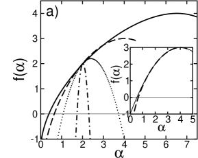
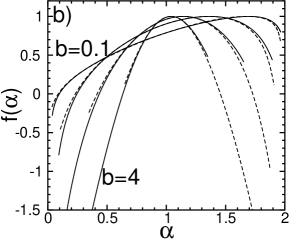
Figure 1: Multifractality at Anderson transitions. a) Singularity spectrum $f(\alpha)$ in $d=2+\epsilon$ for $\epsilon=0.01$ and $\epsilon=0.2$ (analytical), as well as 3D and 4D (numerical). With increasing $d$ the spectrum gets broader, implying stronger multifractality. Inset: comparison between $f(\alpha)$ for 3D and the one-loop result of the $2+\epsilon$ expansion with $\epsilon=1$ (solid).[41] b) Singularity spectrum $f(\alpha)$ for the PRBM model. Evolution from weak to strong multifractality with decreasing parameter $b$ is evident. Dashed lines represent $f(2-\alpha)+\alpha-1$, demonstrating the validity of Eq. (30). [38].

Dimensionality dependence of multifractality

Let us analyze the evolution[41] from the weak-multifractality regime in $d=2+\epsilon$ dimensions to the strong multifractality at $d\gg 1$.

In $2+\epsilon$ dimensions with $\epsilon\ll 1$ the multifractality exponents can be obtained within the $\epsilon$-expansion, Sec. 2. The 4-loop results for the orthogonal and unitary symmetry classes read [42]

$$\Delta_{q}^{(O)} = q(1-q)\epsilon+\frac{\zeta(3)}{4}q(q-1)(q^{2}-q+1)\epsilon^{4}+O(\epsilon^{5});$$ (31)

$$\Delta_{q}^{(U)} = q(1-q)(\epsilon/2)^{1/2}-\frac{3}{8}q^{2}(q-1)^{2}\zeta(3)\epsilon^{2}+O(\epsilon^{5/2}).$$ (32)

Keeping only the leading term on the r.h.s. of Eqs. (31) and (32), we get the one-loop approximation for $\tau_{q}$ which is of parabolic form.

Numerical simulations [41] of the wave function statistics in 3D and 4D (Fig. 1a) have shown a full qualitative agreement with analytical predictions, both in the form of multifractal spectra and in the shape of the IPR distribution. Moreover, the one-loop result of the $2{+}\epsilon$ expansion with $\epsilon{=}1$ describes the 3D singularity spectrum with a remarkable accuracy (though with detectable deviations). In particular, the position of the maximum, $\alpha_{0}{=}4.03{\pm}0.05$, is very close to its value $\alpha_{0}{=}d{+}\epsilon$ implied by one-loop approximation. As expected, in 4D the deviations from parabolic shape are much more pronounced and $\alpha_{0}{=}6.5{\pm}0.2$ differs noticeably from 6.

The simulations[41] also show that fractal dimensions $D_{q}\equiv\tau_{q}/(q-1)$ with $q\gtrsim 1$ decrease with increasing $d$. As an example, for $q=2$ we have $D_{2}\simeq 2-2\epsilon$ in $2+\epsilon$ dimensions, $D_{2}=1.3\pm 0.05$ in 3D, and $D_{2}=0.9\pm 0.15$ in 4D. This confirms the expectation based on the Bethe-lattice results (Sec. 5) that $\tau_{q}\to 0$ at $d\to\infty$ for $q>1/2$. Such a behavior of the multifractal exponents is a manifestation of a very sparse character of critical eigenstates at $d\gg 1$, formed by rare resonance spikes. In combination with the relation (29) this implies the limiting form of the multifractal spectrum at $d\to\infty$,

$$\tau_{q}=\left\{\begin{array}[]{ll}0\ ,&\qquad q\geq 1/2\\ 2d(q-1/2)\ ,&\qquad q\leq 1/2\ .\end{array}\right.$$ (33)

This corresponds to $f(\alpha)$ of the form

$$f(\alpha)=\alpha/2\ ,\qquad 0<\alpha<2d\ ,$$ (34)

dropping to $-\infty$ at the boundaries of the interval $[0,2d]$. It was argued[41] that the way the multifractality spectrum approaches this limiting form with increasing $d$ is analogous to the behavior found[13] in the PRBM model with $b\ll 1$.

Surface vs. bulk multifractality

Recently, the concept of wave function multifractality was extended [43] to the surface of a system at an Anderson transition. It was shown that fluctuations of critical wave functions at the surface are characterized by a new set of exponent $\tau_{q}^{\rm s}$ (or, equivalently, anomalous exponents $\Delta_{q}^{\rm s})$ independent from their bulk counterparts,

$$L^{d-1}\langle|\psi({\bf r})|^{2q}\rangle\sim L^{-\tau_{q}^{\rm s}},$$ (35)

$$\tau_{q}^{\rm s}=d(q-1)+q\mu+1+\Delta_{q}^{\rm s}.$$ (36)

Here $\mu$ is introduced for generality, in order to account for a possibility of non-trivial scaling of the average value, $\langle|\psi({\bf r})|^{2}\rangle\propto L^{-d-\mu}$, at the boundary in unconventional symmetry classes. For the Wigner-Dyson classes, $\mu=0$. The normalization factor $L^{d-1}$ is chosen such that Eq. (35) yields the contribution of the surface to the IPR $\langle P_{q}\rangle=\langle\int d^{d}{\bf r}|\psi({\bf r})|^{2q}\rangle$. The exponents $\Delta_{q}^{\rm s}$ as defined in Eq. (36) vanish in a metal and govern statistical fluctuations of wave functions at the boundary, $\langle|\psi({\bf r})|^{2q}\rangle/\langle|\psi({\bf r})|^{2}\rangle^{q}\sim L^{-\Delta_{q}^{\rm s}}$, as well as their spatial correlations, e.g. $L^{2(d+\mu)}\langle|\psi^{2}({\bf r})\psi^{2}({\bf r}^{\prime})|\rangle\sim(|{\bf r}-{\bf r}^{\prime}|/L)^{\Delta_{2}^{\rm s}}$.

Wave function fluctuations are much stronger at the edge than in the bulk. As a result, surface exponents are important even if one performs a multifractal analysis for the whole sample, without separating it into “bulk” and “surface”, despite the fact that the weight of surface points is down by a factor $1/L$.

The boundary multifractality was explicitly studied, analytically as well as numerically, for a variety of critical systems, including weak multifractality in 2D and $2+\epsilon$ dimensions, the 2D spin quantum Hall transition [43], the Anderson transition in a 2D system with spin-orbit coupling [40], and the PRBM model [38]. The notion of surface multifractality was further generalized[40] to a corner of a critical system.

4 Additional comments

1. For the lack of space we do not discuss the issues of IPR distributions at criticality and the role of ensemble averaging, as well as possible singularities in multifractal spectra, see the review 6.

2. Recently, an impressive progress was achieved in experimental studies of Anderson transitions in various systems.[44, 45, 46, 47, 48] The developed experimental techniques permit spatially resolved investigation of wave functions, thus paving the way to experimental study of multifractality. While the obtained multifractal spectra differ numerically from theoretical expectations (possibly because the systems were not exactly at criticality, or, in the case of electronic systems, pointing to importance of electron-electron interaction), the experimental advances seem very promising.

3. Recent theoretical work[49] explains the properties of a superconductor-insulator transition observed in a class of disordered films in terms of multifractality of electronic wave functions.

5 Anderson transition in $d=\infty$: Bethe lattice

The Bethe lattice (BL) is a tree-like lattice with a fixed coordination number. Since the number of sites at a distance $r$ increases exponentially with $r$ on the BL, it effectively corresponds to the limit of high dimensionality $d$. The BL models are the closest existing analogs of the mean-field theory for the case of the Anderson transition. The Anderson tight-binding model (lattice version of Eqs. (3), (4)) on the BL was studied for the first time in Ref. 50, where the existence of the metal-insulator transition was proven and the position of the mobility edge was determined. Later, the BL versions of the $\sigma$-model (11) [51, 52] and of the tight-binding model [53] were studied within the supersymmetry formalism, which allowed to determine the critical behavior. It was found that the localization length diverges in the way usual for BL models, $\xi\propto|E-E_{c}|^{-1}$, where $E$ is a microscopic parameter driving the transition. When reinterpreted within the effective-medium approximation [54, 55], this yields the conventional mean-field value of the localization length exponent, $\nu=1/2$. On the other hand, the critical behavior of other observables is very peculiar. The inverse participation ratios $P_{q}$ with $q>1/2$ have a finite limit at $E\to E_{c}$ when the critical point is approached from the localized phase and then jump to zero. By comparison with the scaling formula, $P_{q}\propto\xi^{-\tau_{q}}$, this can be interpreted as $\tau_{q}=0$ for all $q\geq 1/2$. Further, in the delocalized phase the diffusion coefficient vanishes exponentially when the critical point is approached,

$$D\propto\Omega^{-1}\ln^{3}\Omega\ ;\qquad\Omega\sim\exp\{{\rm const}\>|E-E_{c}|^{-1/2}\},$$ (37)

which can be thought as corresponding to the infinite value, $s=\infty$, of the critical index $s$. The distribution of the LDOS $v\equiv\rho(r)/\langle\rho\rangle$ (normalized to its average value for convenience) was found to be of the form

$${\cal P}(v)\propto\Omega^{-1/2}v^{-3/2}\ ,\qquad\Omega^{-1}\ll v\ll\Omega\ ,$$ (38)

and exponentially small outside this range. Equation (38) implies for the moments of the LDOS:

$$\langle v^{q}\rangle\propto\Omega^{|q-1/2|-1/2}.$$ (39)

The physical reason for the unconventional critical behavior was unraveled in Ref. 56. It was shown that the exponential largeness of $\Omega$ reflects the spatial structure of the BL: the “correlation volume” $V_{\xi}$ (number of sites within a distance $\xi$ from the given one) on such a lattice is exponentially large. On the other hand, for any finite dimensionality $d$ the correlation volume has a power-law behavior, $V_{d}(\xi)\propto\xi^{d}\propto|E-E_{c}|^{\nu d}$, where $\nu\simeq 1/2$ at large $d$. Thus, the scale $\Omega$ cannot appear for finite $d$ and, assuming some matching between the BL and large-$d$ results, will be replaced by $V_{d}(\xi)$. Then Eq. (39) yields the following high-$d$ behavior of the anomalous exponents $\Delta_{q}$ governing the scaling of the LDOS moments (Sec. 3),

$$\Delta_{q}\simeq d(1/2-|q-1/2|)\ ,$$ (40)

or, equivalently, the results (33), (34) for the multifractal spectra $\tau_{q}$, $f(\alpha)$. These formulas describe the strongest possible multifractality.

The critical behavior of the conductivity, Eq. (37), is governed by the same exponentially large factor $\Omega$. When it is replaced by the correlation volume $V_{d}(\xi)$, the power-law behavior at finite $d\gg 1$ is recovered, $\sigma\propto|E-E_{c}|^{s}$ with $s\simeq d/2$. The result for the exponent $s$ agrees (within its accuracy, i.e. to the leading order in $d$) with the scaling relation $s=\nu(d-2)$.

3 Symmetries of disordered systems

In this section we briefly review the symmetry classification of disordered systems based on the relation to the classical symmetric spaces, which was established in Refs. 7, 8.

1 Wigner-Dyson classes

The random matrix theory (RMT) was introduced into physics by Wigner[57]. Developing Wigner’s ideas, Dyson[58] put forward a classification scheme of ensembles of random Hamiltonians. This scheme takes into account the invariance of the system under time reversal and spin rotations, yielding three symmetry classes: unitary, orthogonal and symplectic. If the time-reversal invariance ($T$) is broken, the Hamiltonians are just arbitrary Hermitian matrices,

$$H=H^{\dagger}\ ,$$ (41)

with no further constraints. This set of matrices is invariant with respect to rotations by unitary matrices; hence the name “unitary ensemble”. In this situation, the presence or absence of spin rotation invariance ($S$) is not essential: if the spin is conserved, $H$ is simply a spinless unitary-symmetry Hamiltonian times the unit matrix in the spin space. In the RMT one considers most frequently an ensemble of matrices with independent, Gaussian-distributed random entries – the Gaussian unitary ensemble (GUE). While disordered systems have much richer physics than the Gaussian ensembles, their symmetry classification is inherited from the RMT.

Let us now turn to the systems with preserved time-reversal invariance. The latter is represented by an antiunitary operator, $T=KC$, where $C$ is the operator of complex conjugation and $K$ is unitary. The time-reversal invariance thus implies $H=KH^{\rm T}K^{-1}$ (we used the Hermiticity, $H^{*}=H^{\rm T}$). Since acting twice with $T$ should leave the physics unchanged, one infers that $K^{*}K=p$, where $p=\pm 1$. As was shown by Wigner, the two cases correspond to systems with integer ($p=+1$) and half-integer ($p=-1$) angular momentum. If $p=1$, a representation can be chosen where $K=1$, so that

$$H=H^{\rm T}\ .$$ (42)

The set of Hamiltonians thus spans the space of real symmetric matrices in this case. This is the orthogonal symmetry class; its representative is the Gaussian orthogonal ensemble (GOE). For disordered electronic systems this class is realized when spin is conserved, as the Hamiltonian then reduces to that for spinless particles (times unit matrix in the spin space).

If $T$ is preserved but $S$ is broken, we have $p=-1$. In the standard representation, $K$ is then realized by the second Pauli matrix, $K=i\sigma_{y}$, so that the Hamiltonian satisfies

$$H=\sigma_{y}H^{\rm T}\sigma_{y}.$$ (43)

It is convenient to split the $2N\times 2N$ Hamiltonian in $2\times 2$ blocks (quaternions) in spin space. Each of them then is of the form $q=q_{0}\sigma_{0}+iq_{1}\sigma_{x}+iq_{2}\sigma_{y}+iq_{3}\sigma_{z}$ (where $\sigma_{0}$ is the unit matrix and $\sigma_{x,y,z}$ the Pauli matrices), with real $q_{\mu}$, which defines a real quaternion. This set of Hamiltonians is invariant with respect to the group of unitary transformations conserving $\sigma_{y}$, $U\sigma_{y}U^{T}=\sigma_{y}$, which is the symplectic group $\text{Sp}(2N)$. The corresponding symmetry class is thus called symplectic, and its RMT representative is the Gaussian symplectic ensemble (GSE).

2 Relation to symmetric spaces

Before discussing the relation to the families of symmetric spaces, we briefly remind the reader how the latter are constructed [59, 60]. Let G be one of the compact Lie groups $\text{SU}(N)$, $\text{SO}(N)$, $\text{Sp}(2N)$, and $\mathfrak{g}$ the corresponding Lie algebra. Further, let $\theta$ be an involutive automorphism $\mathfrak{g}\to\mathfrak{g}$ such that $\theta^{2}=1$ but $\theta$ is not identically equal to unity. It is clear that $\theta$ splits $\mathfrak{g}$ in two complementary subspaces, $\mathfrak{g}=\mathfrak{K}\oplus\mathfrak{P}$, such that $\theta(X)=X$ for $X\in\mathfrak{K}$ and $\theta(X)=-X$ for $X\in\mathfrak{P}$. It is easy to see that the following Lie algebra multiplication relations holds:

$$[\mathfrak{K},\mathfrak{K}]\subset\mathfrak{K},\qquad[\mathfrak{K},\mathfrak{P}]\subset\mathfrak{P},\qquad[\mathfrak{P},\mathfrak{P}]\subset\mathfrak{K}.$$ (44)

This implies, in particular, that $\mathfrak{K}$ is a subalgebra, whereas $\mathfrak{P}$ is not. The coset space $G/K$ (where $K$ is the Lie group corresponding to $\mathfrak{K}$) is then a compact symmetric space. The tangent space to $G/K$ is $\mathfrak{P}$. One can also construct an associated non-compact space. For this purpose, one first defines the Lie algebra $\mathfrak{g}^{*}=\mathfrak{K}\oplus i\mathfrak{P}$, which differs from $\mathfrak{g}$ in that the elements in $\mathfrak{P}$ are multiplied by $i$. Going to the corresponding group and dividing $K$ out, one gets a non-compact symmetric space $G^{*}/K$.

The groups $G$ themselves are also symmetric spaces and can be viewed as coset spaces $G\times G/G$. The corresponding non-compact space is $G^{\mathbb{C}}/G$, where $G^{\mathbb{C}}$ is the complexification of $G$ (which is obtained by taking the Lie algebra $\mathfrak{g}$, promoting it to the algebra over the field of complex numbers, and then exponentiating).

The connection with symmetric spaces is now established in the following way [7, 8]. Consider first the unitary symmetry class. Multiplying a Hamiltonian matrix by $i$, we get an antihermitean matrix $X=iH$. Such matrices form the Lie algebra $\mathfrak{u}(N)$. Exponentiating it, one gets the Lie group $\text{U}(N)$, which is the compact symmetric space of class A in Cartan’s classification. For the orthogonal class, $X=iH$ is purely imaginary and symmetric. The set of such matrices is a linear complement $\mathfrak{P}$ of the algebra $\mathfrak{K}=\mathfrak{o}(N)$ of imaginary antisymmetric matrices in the algebra $\mathfrak{g}=\mathfrak{u}(N)$ of antihermitean matrices. The corresponding symmetric space is $G/K=\text{U}(N)/\text{O}(N)$, which is termed AI in Cartan’s classification. For the symplectic ensemble the same consideration leads to the symmetric space $\text{U}(N)/\text{Sp}(N)$, which is the compact space of the class AII. If we don’t multiply $H$ by $i$ but instead proceed with $H$ in the analogous way, we end up with associated non-compact spaces $G^{*}/K$. To summarize, the linear space $\mathfrak{P}$ of Hamiltonians can be considered as a tangent space to the compact $G/K$ and non-compact $G^{*}/K$ symmetric spaces of the appropriate symmetry class.

Symmetry classification of disordered systems. First column: symbol for the symmetry class of the Hamiltonian. Second column: names of the corresponding RMT. Third column: presence (+) or absence ($-$) of the time-reversal (T) and spin-rotation (S) invariance. Fourth and fifth columns: families of the compact and non-compact symmetric spaces of the corresponding symmetry class. The Hamiltonians span the tangent space to these symmetric spaces. Sixth column: symmetry class of the $\sigma$-model; the first symbol corresponds to the non-compact (“bosonic”) and the second to the compact (“fermionic”) sector of the base of the $\sigma$-model manifold. The compact component ${\cal M}_{F}$ (which is particularly important for theories with non-trivial topological properties) is explicitly given in the last column. From Ref. 6 Ham. RMT T    S compact non-compact $\sigma$-model $\sigma$-model compact class symmetric space symmetric space B$|$F sector ${\cal M}_{F}$ Wigner-Dyson classes A GUE $-$    $\pm$ $\text{U}(N){\times}\text{U}(N)/\text{U}(N)\equiv\text{U}(N)$ $\text{GL}(N,\mathbb{C})/\text{U}(N)$ AIII$|$AIII $\text{U}(2n)/\text{U}(n){\times}\text{U}(n)$ AI GOE $+$   $+$ $\text{U}(N)/\text{O}(N)$ $\text{GL}(N,\mathbb{R})/\text{O}(N)$ BDI$|$CII $\text{Sp}(4n)/\text{Sp}(2n){\times}\text{Sp}(2n)$ AII GSE $+$   $-$ $\text{U}(2N)/\text{Sp}(2N)$ $\text{U}^{*}(2N)/\text{Sp}(2N)$ CII$|$BDI $\text{O}(2n)/\text{O}(n){\times}\text{O}(n)$ chiral classes AIII chGUE $-$    $\pm$ $\text{U}(p+q)/\text{U}(p){\times}\text{U}(q)$ $\text{U}(p,q)/\text{U}(p){\times}\text{U}(q)$ A$|$A $\text{U}(n)$ BDI chGOE $+$   $+$ $\text{SO}(p+q)/\text{SO}(p){\times}\text{SO}(q)$ $\text{SO}(p,q)/\text{SO}(p){\times}\text{SO}(q)$ AI$|$AII $\text{U}(2n)/\text{Sp}(2n)$ CII chGSE $+$   $-$ $\text{Sp}(2p+2q)/\text{Sp}(2p){\times}\text{Sp}(2q)$ $\text{Sp}(2p,2q)/\text{Sp}(2p){\times}\text{Sp}(2q)$ AII$|$AI $\text{U}(n)/\text{O}(n)$ Bogoliubov - de Gennes classes C $-$    $+$ $\text{Sp}(2N){\times}\text{Sp}(2N)/\text{Sp}(2N)\equiv\text{Sp}(2N)$ $\text{Sp}(2N,\mathbb{C})/\text{Sp}(2N)$ DIII$|$CI $\text{Sp}(2n)/\text{U}(n)$ CI $+$    $+$ $\text{Sp}(2N)/\text{U}(N)$ $\text{Sp}(2N,\mathbb{R})/\text{U}(N)$ D$|$C $\text{Sp}(2n)$ BD $-$    $-$ $\text{SO}(N){\times}\text{SO}(N)/\text{SO}(N)\equiv\text{SO}(N)$ $\text{SO}(N,\mathbb{C})/\text{SO}(N)$ CI$|$DIII $\text{O}(2n)/\text{U}(n)$ DIII $+$    $-$ $\text{SO}(2N)/\text{U}(N)$ $\text{SO}^{*}(2N)/\text{U}(N)$ C$|$D $\text{O}(n)$

This correspondence is summarized in Table 2, where the first three rows correspond to the Wigner-Dyson classes, the next three to the chiral classes (Sec. 3) and last four to the Bogoliubov-de Gennes classes (Sec. 4). The last two columns of the table specify the symmetry of the corresponding $\sigma$-model. In the supersymmetric formulation, the base of the $\sigma$-model target space $\cal{M}_{B}\times\cal{M}_{F}$ is the product of a non-compact symmetric space $\cal{M}_{B}$ corresponding to the bosonic sector and a compact (“fermionic”) symmetric space $\cal{M}_{F}$. (In the replica formulation, the space is $\cal{M}_{B}$ for bosonic or $\cal{M}_{F}$ for fermionic replicas, supplemented with the limit $n\to 0$.) The Cartan symbols for these symmetric spaces are given in the sixth column, and the compact components $\cal{M}_{F}$ are listed in the last column. It should be stressed that the symmetry classes of $\cal{M}_{B}$ and $\cal{M}_{F}$ are different from the symmetry class of the ensemble (i.e. of the Hamiltonian) and in most cases are also different from each other. Following the common convention, when we refer to a system as belonging to a particular class, we mean the symmetry class of the Hamiltonian.

It is also worth emphasizing that the orthogonal groups appearing in the expressions for $\cal{M}_{F}$ are $\text{O}(N)$ rather than $\text{SO}(N)$. This difference (which was irrelevant when we were discussing the symmetry of the Hamiltonians, as it does not affect the tangent space) is important here, since it influences topological properties of the manifold. As we will detail in Sec. 4,6, the topology of the $\sigma$-model target space often affects the localization properties of the theory in a crucial way.

3 Chiral classes

The Wigner-Dyson classes are the only allowed if one looks for a symmetry that is translationally invariant in energy, i.e. is not spoiled by adding a constant to the Hamiltonian. However, additional discrete symmetries may arise at some particular value of energy (which can be chosen to be zero without loss of generality), leading to novel symmetry classes. As the vicinity of a special point in the energy space governs the physics in many cases (i.e. the band center in lattice models at half filling, or zero energy in gapless superconductors), these ensembles are of large interest. They can be subdivided into two groups – chiral and Bogoliubov - de Gennes ensembles – considered here and in Sec. 4, respectively.

The chiral ensembles appeared in both contexts of particle physics and physics of disordered electronic systems about fifteen years ago [62, 63, 64, 65]. The corresponding Hamiltonians have the form

$${H}=\left(\begin{array}[]{cc}0&h\\ h^{\dagger}&0\end{array}\right)\ ,$$ (45)

i.e. they possess the symmetry

$$\tau_{z}H\tau_{z}=-H\ ,$$ (46)

where $\tau_{z}$ is the third Pauli matrix in a certain “isospin” space. In the condensed matter context, such ensembles arise, in particular, when one considers a tight-binding model on a bipartite lattice with randomness in hopping matrix elements only. In this case, $H$ has the block structure (45) in the sublattice space.

In addition to the chiral symmetry, a system may possess time reversal and/or spin-rotation invariance. In full analogy with the Wigner-Dyson classes, 1, one gets therefore three chiral classes (unitary, orthogonal, and symplectic). The corresponding symmetric spaces, the Cartan notations for symmetry classes, and the $\sigma$-model manifolds are given in the rows 4–6 of the Table 2.

4 Bogoliubov - de Gennes classes

The Wigner-Dyson and chiral classes do not exhaust all possible symmetries of disordered electronic systems[7]. The remaining four classes arise most naturally in superconducting systems. The quasiparticle dynamics in such systems can be described by the Bogoliubov-de Gennes Hamiltonian of the form

$$\hat{H}=\sum_{\alpha\beta}^{N}h_{\alpha\beta}c^{\dagger}_{\alpha}c_{\beta}+\frac{1}{2}\sum_{\alpha\beta}^{N}\left(\Delta_{\alpha\beta}c^{\dagger}_{\alpha}c^{\dagger}_{\beta}-\Delta_{\alpha\beta}^{*}c_{\alpha}c_{\beta}\right),$$ (47)

where $c^{\dagger}$ and $c$ are fermionic creation and annihilation operators, and the $N\times N$ matrices $h$, $\Delta$ satisfy $h=h^{\dagger}$ and $\Delta^{T}=-\Delta$, in view of hermiticity. Combining $c^{\dagger}_{\alpha},c_{\alpha}$ in a spinor $\psi_{\alpha}^{\dagger}=(c_{\alpha}^{\dagger},c_{\alpha})$, one gets a matrix representation of the Hamiltonian, $\hat{H}=\psi^{\dagger}H\psi$, where

$$H=\left(\begin{array}[]{cc}h&\Delta\\ -\Delta^{*}&-h^{T}\end{array}\right),\qquad h=h^{\dagger}\ ,\ \ \Delta=-\Delta^{T}\ .$$ (48)

The minus signs in the definition of $H$ result form the fermionic commutation relations between $c^{\dagger}$ and $c$. The Hamiltonian structure (48) corresponds to the condition

$$H=-\tau_{x}H^{T}\tau_{x}$$ (49)

(in addition to the Hermiticity $H=H^{\dagger}$), where $\tau_{x}$ is the Pauli matrix in the particle-hole space. Alternatively, one can perform a unitary rotation of the basis, defining $\tilde{H}=g^{\dagger}Hg$ with $g=(1+i\tau_{x})/\sqrt{2}$. In this basis, the defining condition of class D becomes $\tilde{H}=-\tilde{H}^{T}$, so that $\tilde{H}$ is pure imaginary. The matrices $X=iH$ thus form the Lie algebra $\mathfrak{so}(2N)$, corresponding to the Cartan class D. This symmetry class described disordered superconducting systems in the absence of other symmetries.

Again, the symmetry class will be changed if the time reversal and/or spin rotation invariance are present. The difference with respect to the Wigner-Dyson and chiral classes is that now one gets four different classes rather than three. This is because the spin-rotation invariance has an impact even in the absence of time-reversal invariance, since it combines with the particle-hole symmetry in a non-trivial way. Indeed, if the spin is conserved, the Hamiltonian has the form

$$\hat{H}=\sum_{ij}^{N}\left[h_{ij}(c_{i\uparrow}^{\dagger}c_{j\uparrow}-c_{j\downarrow}c^{\dagger}_{i,\downarrow})+\Delta_{ij}c^{\dagger}_{i,\uparrow}c^{\dagger}_{j,\downarrow}+\Delta^{*}_{ij}c_{i\downarrow}c_{j\uparrow}\right],$$ (50)

where $h$ and $\Delta$ are $N{\times}N$ matrices satisfying $h=h^{\dagger}$ and $\Delta=\Delta^{T}$. Similar to (48), we can introduce the spinors $\psi_{i}^{\dagger}=(c_{i\uparrow}^{\dagger},c_{i\downarrow})$ and obtain the following matrix form of the Hamiltonian

$${H}=\left(\begin{array}[]{cc}{h}&{\Delta}\\ {\Delta}^{*}&{-h}^{T}\end{array}\right),\qquad h=h^{\dagger}\ ,\ \ \Delta=\Delta^{T}\ .$$ (51)

It exhibits a symmetry property

$$H=-\tau_{y}H^{T}\tau_{y}.$$ (52)

The matrices $H=iX$ now form the Lie algebra $\mathfrak{sp}(2N)$, which is the symmetry class C.

If the time reversal invariance is present, one gets two more classes (CI and DIII). The symmetric spaces for the Hamiltonians and the $\sigma$-models corresponding to the Bogoliubov–de Gennes classes are given in the last four rows of the Table 2.

The following comment is in order here. Strictly speaking, one should distinguish between the orthogonal group $\mathrm{SO}(N)$ with even and odd $N$, which form different Cartan classes: $\mathrm{SO}(2N)$ belongs to class D, while $\mathrm{SO}(2N{+}1)$ to class B. In the conventional situation of a disordered superconductor, the matrix size is even due to the particle-hole space doubling, see Sec. 4. It was found, however, that the class B can arise in $p$-wave vortices [75]. In the same sense, the class DIII should be split in DIII-even and DIII-odd; the last one represented by the symmetric space $\text{SO}(4N+2)/\text{U}(2N+1)$ can appear in vortices in the presence of time-reversal symmetry.

5 Perturbative RG for $\sigma$-models of different symmetry classes

Perturbative $\beta$-functions for $\sigma$-models on all the types of symmetric spaces were in fact calculated [26, 27] long before the physical significance of the chiral and Bogoliubov-de Gennes classes has been fully appreciated. These results are important for understanding the behavior of systems of different symmetry classes in 2D. (We should emphasize once more, however, that this does not give a complete information about all possible types of criticality since the latter can be crucially affected by additional terms of topological character in the $\sigma$-model, see Sec. 4, 6 below.)

One finds that in the classes A, AI, C, CI the $\beta$-function is negative in 2D in the replica limit (at least, for small $t$). This indicates that normally all states are localized in such systems in 2D. (This conclusion can in fact be changed in the presence of topological or Wess-Zumino terms, Sec. 1.) Above 2D, these systems undergo the Anderson transition that can be studied within the $2+\epsilon$ expansion, Sec. 2. For the classes AIII, BDI, and CII (chiral unitary, orthogonal and symplectic classes, respectively) the $\beta(t)\equiv 0$ in 2D, implying a line of fixed points. Finally, in the classes AII, D, and DIII the $\beta$-function is positive at small $t$, implying the existence of a metal-insulator transition at strong coupling in 2D.

4 Criticality in 2D

1 Mechanisms of criticality in 2D

As was discussed in Sec. 2, conventional Anderson transitions in the orthogonal and unitary symmetry classes take place only if the dimensionality is $d>2$, whereas in 2D all states are localized. It is, however, well understood by now that there is a rich variety of mechanisms that lead to emergence of criticality in 2D disordered systems.[61] Such 2D critical points have been found to exist for 9 out of 10 symmetry classes, namely, in all classes except for the orthogonal class AI. A remarkable peculiarity of 2D critical points is that the critical conductance $g_{*}$ is at the same time the critical conductivity. We now list and briefly describe the mechanisms for the emergence of criticality.

Broken spin-rotation invariance: Metallic phase

We begin with the mechanism that has been already mentioned in Sec. 2 in the context of the Wigner-Dyson symplectic class (AII). In this case the $\beta$-function [(19) with $\epsilon=0$] is positive for not too large $t$ (i.e. sufficiently large conductance), so that the system is metallic ($t$ scales to zero under RG). On the other hand, for strong disorder (low $t$) the system is an insulator, as usual, i.e. $\beta(t)<0$. Thus, $\beta$-function crosses zero at some $t_{*}$, which is a point of the Anderson transition.

This mechanism (positive $\beta$-function and, thus, metallic phase at small $t$, with a transition at some $t_{*}$) is also realized in two of Bogoliubov-de Gennes classes – D and DIII. All these classes correspond to systems with broken spin-rotation invariance. The unconventional sign of the $\beta$-function in these classes, indicating weak antilocalization (rather then localization), is physically related to destructive interference of time reversed paths for particles with spin $s=1/2$.

Chiral classes: Vanishing $\beta$-function

Another peculiarity of the perturbative $\beta$-function takes place for three chiral classes – AIII, BDI, ad CII. Specifically, for these classes $\beta(t)\equiv 0$ to all orders of the perturbation theory, as was first discovered by Gade and Wegner [63, 62]. As a result, the conductance is not renormalized at all, serving as an exactly marginal coupling. There is thus a line of critical points for these models, labeled by the value of the conductance. In fact, the $\sigma$-models for these classes contain an additional term [63, 62] that does not affect the absence of renormalization of the conductance but is crucial for the analysis of the behavior of the DOS.

Broken time-reversal invariance: Topological $\theta$-term and quantum Hall criticality

For several classes, the $\sigma$-model action allows for inclusion of a topological term, which is invisible to any order of the perturbation theory. This is the case when the second homotopy group $\pi_{2}$ of the $\sigma$-model manifold ${\cal M}$ (a group of homotopy classes of maps of the sphere $S^{2}$ into ${\cal M}$) is non-trivial. From this point of view, only the compact sector ${\cal M}_{F}$ (originating from the fermionic part of the supervector field) of the manifold base matters. There are five classes, for which $\pi_{2}({\cal M}_{F})$ is non-trivial, namely A, C, D, AII, and CII.

For the classes A, C, D the homotopy group $\pi_{2}({\cal M}_{F})=\mathbb{Z}$. Therefore, the action $S[Q]$ may include the (imaginary) $\theta$-term,

$$iS_{\rm top}[Q]=i\theta N[Q]\ ,$$ (53)

where an integer $N[Q]$ is the winding number of the field configuration $Q({\bf r})$. Without loss of generality, $\theta$ can be restricted to the interval $[0,2\pi]$, since the theory is periodic in $\theta$ with the period $2\pi$.

The topological term (53) breaks the time reversal invariance, so it may only arise in the corresponding symmetry classes. The by far most famous case is the Wigner-Dyson unitary class (A). As was first understood by Pruisken[9], the $\sigma$-model of this class with the topological term (53) describes the integer quantum Hall effect (IQHE), with the critical point of the plateau transition corresponding to $\theta{=}\pi$. More recently, it was understood that counterparts of the IQHE exist also in the Bogoliubov-de Gennes classes with broken time-reversal invariance – classes C[66, 67, 68, 69, 70] and D.[71, 72, 79, 73, 74] They were called spin and thermal quantum Hall effects (SQHE and TQHE), respectively.

$\mathbb{Z}_{2}$ topological term

For two classes, AII and CII, the second homotopy group is $\pi_{2}({\cal M}_{F})=\mathbb{Z}_{2}$. This allows for the $\theta$-term but $\theta$ can only take the values $0$ and $\pi$. It has been recently shown [88] that the $\sigma$-model of the Wigner-Dyson symplectic class (AII) with a $\theta{=}\pi$ topological angle arises from a model of Dirac fermions with random scalar potential, which describes, in particular, graphene with long-range disorder. Like in the case of quantum-Hall systems, this topological term inhibits localization.

Wess-Zumino term

Finally, one more mechanism of emergence of criticality is the Wess-Zumino (WZ) term that may appear in $\sigma$-models of the classes AIII, CI, and DIII. For these classes, the compact component ${\cal M}_{F}$ of the manifold is the group $H\times H/H=H$, where $H$ is $\text{U}(n)$, $\text{Sp}(2n)$, and $\text{O}(2n)$, respectively. The corresponding theories are called “principal chiral models”. The WZ term has the following form:

$$iS_{\rm WZ}(g)=\frac{ik}{24\pi}\int d^{2}r\int_{0}^{1}ds\>\epsilon_{\mu\nu\lambda}{\rm Str}(g^{-1}\partial_{\mu}g)(g^{-1}\partial_{\nu}g)(g^{-1}\partial_{\lambda}g),$$ (54)

where $k$ is an integer called the level of the WZW model. The definition (54) of the WZ term requires an extension of the $\sigma$-model field $g({\bf r})\equiv g(x,y)$ to the third dimension, $0\leq s\leq 1$, such that $g({\bf r},0)=1$ and $g({\bf r},1)=g({\bf r})$. Such an extension is always possible, since the second homotopy group is trivial, $\pi_{2}(H)=0$, for all the three classes. Further, the value of the WZ term does not depend on the particular way the extension to the third dimension is performed. (This becomes explicit when one calculates the variation of the WZ term: it is expressed in terms of $g({\bf r})$ only.) More precisely, there is the following topological ambiguity in the definition of $S_{\rm WZ}(g)$. Since the third homotopy group is non-trivial, $\pi_{3}(H)=\mathbb{Z}$, $S_{\rm WZ}(g)$ is defined up to an arbitrary additive integer $n$ times $2\pi k$. This, however, does not affect any observables, since simply adds the phase $nk\times 2\pi i$ to the action.

The WZ term arises when one bosonizes certain models of Dirac fermions [76] and is a manifestation of the chiral anomaly. In particular, a $\sigma$-model for a system of the AIII (chiral unitary) class with the WZ term describes Dirac fermions in a random vector potential. In this case the $\sigma$-model coupling constant is truly marginal (as is typical for chiral classes) and one finds a line of fixed points. On the other hand, for the class CI there is a single fixed point. The WZW models of these classes were encountered in the course of study of dirty $d$-wave superconductors [77, 78] and, most recently, in the context of disordered graphene. We will discuss critical properties of these models in Sec. 2.

2 Disordered Dirac Hamiltonians and graphene

Localization and criticality in models of 2D Dirac fermions subjected to various types of disorder have been studied in a large number of papers and in a variety of contexts, including the random bond Ising model [80], the quantum Hall effect [83], dirty superconductors with unconventional pairing [77, 79, 78], and some lattice models with chiral symmetry [81]. Recently, this class of problems has attracted a great deal of attention[82, 84, 85, 86, 87, 88, 89] in connection with its application to graphene.[91, 92]

One of the most prominent experimentally discovered features of graphene is the “minimal conductivity” at the neutrality (Dirac) point. Specifically, the conductivity[93, 94, 95] of an undoped sample is close to $e^{2}/h$ per spin per valley, remaining almost constant in a very broad temperature range—from room temperature down to 30mK. This is in contrast with conventional 2D systems driven by Anderson localization into insulating state at low $T$ and suggests that delocalization (and, possibly, quantum criticality) may emerge in a broad temperature range due to special character of disordered graphene Hamiltonian.

In the presence of different types of randomness, Dirac Hamiltonians realize all ten symmetry classes of disordered systems; see Ref. 90 for a detailed symmetry classification. Furthermore, in many cases the Dirac character of fermions induces non-trivial topological properties ($\theta$-term or WZ term) of the corresponding field theory ($\sigma$-model). In Sec. 2 we review the classification of disorder in a two-flavor model of Dirac fermions describing the low-energy physics of graphene and types of criticality. The emergent critical theories will be discussed in Sec. 2–2.

Symmetries of disorder and types of criticality.

The presentation below largely follows Refs. 87, 89. We concentrate on a two-flavor model, which is in particular relevant to the description of electronic properties of graphene. Graphene is a semimetal; its valence and conduction bands touch each other in two conical points $K$ and $K^{\prime}$ of the Brillouin zone. In the vicinity of these points the electrons behave as massless relativistic (Dirac-like) particles. Therefore, the effective tight-binding low-energy Hamiltonian of clean graphene is a $4\times 4$ matrix operating in the $AB$ space of the two sublattices and in the $K$–$K^{\prime}$ space of the valleys:

$$H=v_{0}\tau_{3}\bm{\sigma}\mathbf{k}.$$ (55)

Here $\tau_{3}$ is the third Pauli matrix in the $K$–$K^{\prime}$ space, $\bm{\sigma}=\{\sigma_{1},\sigma_{2}\}$ the two-dimensional vector of Pauli matrices in the $AB$ space, and $v_{0}$ the velocity ($v_{0}\simeq 10^{8}$ cm/s in graphene). It is worth emphasizing that the Dirac form of the Hamiltonian (55) does not rely on the tight-binding approximation but is protected by the symmetry of the honeycomb lattice which has two atoms in a unit cell.

Let us analyze the symmetries of the clean Hamiltonian (55) in the $AB$ and $KK^{\prime}$ spaces. First, there exists an SU(2) symmetry group in the space of the valleys, with the generators [82]

$$\Lambda_{x}=\sigma_{3}\tau_{1},\qquad\Lambda_{y}=\sigma_{3}\tau_{2},\qquad\Lambda_{z}=\sigma_{0}\tau_{3}\ ,$$ (56)

all of which commute with the Hamiltonian. Second, there are two more symmetries of the clean Hamiltonian, namely, time inversion operation ($T_{0}$) and chiral symmetry ($C_{0}$). Combining $T_{0}$, $C_{0}$, and isospin rotations $\Lambda_{0,x,y,z}$, one can construct twelve symmetry operations, out of which four (denoted as $T_{\mu}$) are of time-reversal type, four ($C_{\mu}$) of chiral type, and four ($CT_{\mu}$) of Bogoliubov-de Gennes type:

$$T_{0}:\ A\mapsto\sigma_{1}\tau_{1}A^{T}\sigma_{1}\tau_{1},\ \ \ C_{0}:\ A\mapsto-\sigma_{3}\tau_{0}A\sigma_{3}\tau_{0},\ \ \ CT_{0}:\ A\mapsto-\sigma_{2}\tau_{1}A^{T}\sigma_{2}\tau_{1},$$

$$T_{x}:\ A\mapsto\sigma_{2}\tau_{0}A^{T}\sigma_{2}\tau_{0},\ \ \ C_{x}:\ A\mapsto-\sigma_{0}\tau_{1}A\sigma_{0}\tau_{1},\ \ \ CT_{x}:\ A\mapsto-\sigma_{1}\tau_{0}A^{T}\sigma_{1}\tau_{0},$$

$$T_{y}:\ A\mapsto\sigma_{2}\tau_{3}A^{T}\sigma_{2}\tau_{3},\ \ \ C_{y}:\ A\mapsto-\sigma_{0}\tau_{2}A\sigma_{0}\tau_{2},\ \ \ CT_{y}:\ A\mapsto-\sigma_{1}\tau_{3}A^{T}\sigma_{1}\tau_{3},$$

$$T_{z}:\ A\mapsto\sigma_{1}\tau_{2}A^{T}\sigma_{1}\tau_{2},\ \ \ C_{z}:\ A\mapsto-\sigma_{3}\tau_{3}A\sigma_{3}\tau_{3},\ \ \ CT_{z}:\ A\mapsto-\sigma_{2}\tau_{2}A^{T}\sigma_{2}\tau_{2}.$$

It is worth recalling that the $C$ and $CT$ symmetries apply to the Dirac point ($E=0$), i.e. to undoped graphene, and get broken by a non-zero energy $E$. We will assume the average isotropy of the disordered graphene, which implies that $\Lambda_{x}$ and $\Lambda_{y}$ symmetries of the Hamiltonian are present or absent simultaneously. They are thus combined into a single notation $\Lambda_{\perp}$; the same applies to $T_{\perp}$ and $C_{\perp}$. In Table 2 all possible matrix structures of disorder along with their symmetries are listed.

Disorder symmetries in graphene. The first five rows represent disorders preserving the time reversal symmetry $T_{0}$; the last four — violating $T_{0}$. First column: structure of disorder in the sublattice ($\sigma_{\mu}$) and valley ($\tau_{\nu}$) spaces. The remaining columns indicate which symmetries of the clean Hamiltonian are preserved by disorder. [87]. structure $\Lambda_{\perp}$ $\Lambda_{z}$ $T_{0}$ $T_{\perp}$ $T_{z}$ $C_{0}$ $C_{\perp}$ $C_{z}$ $CT_{0}$ $CT_{\perp}$ $CT_{z}$ $\sigma_{0}\tau_{0}$ $+$ $+$ $+$ $+$ $+$ $-$ $-$ $-$ $-$ $-$ $-$ $\sigma_{\{1,2\}}\tau_{\{1,2\}}$ $-$ $-$ $+$ $-$ $-$ $+$ $-$ $-$ $+$ $-$ $-$ $\sigma_{1,2}\tau_{0}$ $-$ $+$ $+$ $-$ $+$ $+$ $-$ $+$ $+$ $-$ $+$ $\sigma_{0}\tau_{1,2}$ $-$ $-$ $+$ $-$ $-$ $-$ $-$ $+$ $-$ $-$ $+$ $\sigma_{3}\tau_{3}$ $-$ $+$ $+$ $-$ $+$ $-$ $+$ $-$ $-$ $+$ $-$ $\sigma_{3}\tau_{1,2}$ $-$ $-$ $-$ $-$ $+$ $-$ $-$ $+$ $+$ $-$ $-$ $\sigma_{0}\tau_{3}$ $-$ $+$ $-$ $+$ $-$ $-$ $+$ $-$ $+$ $-$ $+$ $\sigma_{1,2}\tau_{3}$ $+$ $+$ $-$ $-$ $-$ $+$ $+$ $+$ $-$ $-$ $-$ $\sigma_{3}\tau_{0}$ $+$ $+$ $-$ $-$ $-$ $-$ $-$ $-$ $+$ $+$ $+$

If all types of disorder are present (i.e. no symmetries is preserved), the RG flow is towards the conventional localization fixed point (unitary Wigner-Dyson class A). If the only preserved symmetry is the time reversal ($T_{0}$), again the conventional localization (orthogonal Wigner-Dyson class AI) takes place [85]. A non-trivial situation occurs if either (i) one of the chiral symmetries is preserved or (ii) the valleys remain decoupled. In Table 2 we list situations when symmetry prevents localization and leads to criticality and non-zero conductivity at $E{=}0$ (in the case of decoupled nodes – also at nonzero $E$). Models with decoupled nodes are analyzed in Sec. 2, and models with a chiral symmetry in Sec. 2 ($C_{0}$-chirality) and 2 ($C_{z}$-chirality).

Possible types of disorder in graphene leading to criticality. The first three row correspond to $C_{z}$ chiral symmetry leading to Gade-Wegner-type criticality, Sec. 2. The next three rows contain models with $C_{0}$ chiral symmetry (random gauge fields), inducing a WZ term in the $\sigma$-model action, Sec. 2. The last four rows correspond to the case of decoupled valleys (long-range disorder), see Sec. 2; In the last three cases the $\sigma$-model acquires a topological term with $\theta=\pi$. Adapted from Ref. 89. Disorder Symmetries Class Criticality Conductivity Vacancies, strong potential impurities $C_{z}$, $T_{0}$ BDI Gade $\approx 4e^{2}/\pi h$ Vacancies + RMF $C_{z}$ AIII Gade $\approx 4e^{2}/\pi h$ $\sigma_{3}\tau_{1,2}$ disorder $C_{z}$, $T_{z}$ CII Gade $\approx 4e^{2}/\pi h$ Dislocations $C_{0}$, $T_{0}$ CI WZW $4e^{2}/\pi h$ Dislocations + RMF $C_{0}$ AIII WZW $4e^{2}/\pi h$ Ripples, RMF $\Lambda_{z}$, $C_{0}$ $2\times$AIII WZW $4e^{2}/\pi h$ Charged impurities $\Lambda_{z}$, $T_{\perp}$ $2\times$AII $\theta=\pi$ $4\sigma_{Sp}^{**}$ or${}^{\text{a}}$ $(4e^{2}/\pi h)\ln L$ Random Dirac mass: $\sigma_{3}\tau_{0}$, $\sigma_{3}\tau_{3}$ $\Lambda_{z}$, $CT_{\perp}$ $2\times$D $\theta=\pi$ $4e^{2}/\pi h$ Charged impurities + (RMF, ripples) $\Lambda_{z}$ $2\times$A $\theta=\pi$ $4\sigma_{U}^{*}$ ${}^{\text{a}}$Numerical simulations[96] reveal a flow towards the supermetal fixed point, $\sigma\simeq(4e^{2}/\pi h)\ln L\to\infty$.

Decoupled nodes: Disordered single-flavor Dirac fermions and quantum-Hall-type criticality

If the disorder is of long-range character, the valley mixing is absent due to the lack of scattering with large momentum transfer. For each of the nodes, the system can then be described in terms of a single-flavor Dirac Hamiltonian,

$$H=v_{0}[\bm{\sigma}\mathbf{k}+\sigma_{\mu}V_{\mu}(\mathbf{r})].$$ (57)

Here disorder includes random scalar ($V_{0}$) and vector ($V_{1,2}$) potentials and random mass ($V_{3}$). The clean single-valley Hamiltonian (57) obeys the effective time-reversal invariance $H=\sigma_{2}H^{T}\sigma_{2}$. This symmetry ($T_{\perp}$) is not the physical time-reversal symmetry ($T_{0}$): the latter interchanges the nodes and is of no significance in the absence of inter-node scattering.

Remarkably, single-flavor Dirac fermions are never in the conventional localized phase! More specifically, depending on which of the disorders are present, four different types of criticality take place:

(i) The only disorder is the random vector potential ($V_{1,2}$). This is a special case of the symmetry class AIII. This problem is exactly solvable. It is characterized by a line of fixed points, all showing conductivity $4e^{2}/\pi h$, see Sec. 2.

(ii) Only random mass ($V_{3}$) is present. The system belongs then to class D. The random-mass disorder is marginally irrelevant, and the system flows under RG towards the clean fixed point, with the conductivity $4e^{2}/\pi h$.

(iii) The only disorder is random scalar potential ($V_{0}$). The system is then in the Wigner-Dyson symplectic (AII) symmetry class. As was found in Ref. 88, the corresponding $\sigma$-model contains a $\mathbb{Z}_{2}$ topological term with $\theta=\pi$ which protects the system from localization. The absence of localization in this model has been confirmed in numerical simulations.[96] The scaling function has been found in Ref. 96 to be strictly positive, implying a flow towards the “supermetal” fixed point.

(iv) At least two types of randomness are present. All symmetries are broken in this case and the model belongs to the Wigner-Dyson unitary class A. It was argued in Ref. 83 that it flows into the IQH transition fixed point. This is confirmed by the derivation of the corresponding $\sigma$-model [78, 88, 89], which contains a topological term with $\theta=\pi$, i.e. is nothing but the Pruisken $\sigma$-model at criticality. A particular consequence of this is that the conductivity of graphene with this type of disorder is equal to the value $\sigma_{U}^{*}$ of the longitudinal conductivity $\sigma_{xx}$ at the critical point of the IQH transition multiplied by four (because of spin and valleys).

If a uniform transverse magnetic field is applied, the topological angle $\theta$ becomes energy-dependent. However, at the Dirac point ($E=0$), where $\sigma_{xy}=0$, its value remains unchanged, $\theta=\pi$. This implies the emergence of the half-integer quantum Hall effect, with a plateau transition point at $E=0$.

Preserved $C_{0}$ chirality: Random gauge fields

Let us consider a type of disorder which preserves the $C_{0}$-chirality, $H=-\sigma_{3}H\sigma_{3}$. This implies the disorder of the type $\sigma_{1,2}\tau_{0,1,2,3}$ being strictly off-diagonal in the $\sigma$ space. Depending on further symmetries, three different $C_{0}$-chiral models arise:

(i) The only disorder present is $\sigma_{1,2}\tau_{3}$, which corresponds to the random abelian vector potential. In this case the nodes are decoupled, and the Hamiltonian decomposes in two copies of a model of the class AIII. This model characterized by a line of fixed points has already been mentioned in Sec.2.

(ii) If the time-reversal symmetry $T_{0}$ is preserved, only the disorder of the type $\sigma_{1,2}\tau_{0,1,2}$ is allowed, and the problem is in the symmetry class CI. The model describes then fermions coupled to a SU(2) non-abelian gauge field, and is a particular case of analogous SU(N) models. This theory flows now into an isolated fixed point, which is a WZW theory on the level $k=-2N$.[77, 35, 97]

(iii) All $C_{0}$-invariant disorder structures are present. This describes Dirac fermions coupled to both abelian U(1) and non-abelian SU(2) gauge fields. This model is in the AIII symmetry class.

Remarkably, all these critical $C_{0}$-chiral models are exactly solvable. In particular, the critical conductivity can be calculated exactly and is independent on the disorder strength. A general proof of this statement based only on the gauge invariance is given in Ref. 87. (For particular cases it was earlier obtained in Refs.83, 98). The critical conductivity is thus the same as in clean graphene,

$$\sigma=4e^{2}/\pi h.$$ (58)

Spectra of multifractal exponents and the critical index of the DOS can also be calculated exactly, see the review[6].

Disorders preserving $C_{z}$ chirality: Gade-Wegner criticality

Let us now turn to the disorder which preserves the $C_{z}$-chirality, $H=-\sigma_{3}\tau_{3}H\sigma_{3}\tau_{3}$; according to Table 2, the corresponding disorder structure is $\sigma_{1,2}\tau_{0,3}$ and $\sigma_{0,3}\tau_{1,2}$ If no time-reversal symmetries are preserved, the system belongs to the chiral unitary (AIII) class. The combination of $C_{z}$-chirality and the time reversal invariance $T_{0}$ corresponds to the chiral orthogonal symmetry class BDI; this model has already been discussed in Sec. 1. Finally, the combination of $C_{z}$-chirality and $T_{z}$-symmetry falls into the chiral symplectic symmetry class CII. The RG flow and DOS in these models have been analyzed in Ref. 81 In all the cases, the resulting theory is of the Gade-Wegner type.[63, 62] These theories are characterized by lines of fixed points, with non-universal conductivity. It was found[87, 100] that for weak disorder the conductivity takes approximately the universal value, $\sigma\simeq 4e^{2}/\pi h$. In contrast to the case of $C_{0}$ chirality, this result is, however, not exact. In particular, the leading correction to the clean conductivity is found in the second order in disorder strength[87].

5 Electron-electron-interaction effects

Physically, the impact of interaction effects onto low-temperature transport and localization in disordered electronic systems can be subdivided into two distinct effects: (i) renormalization and (ii) dephasing.

Renormalization.

The renormalization effects, which are governed by virtual processes, become increasingly more pronounced with lowering temperature. The importance of such effects in diffusive low-dimensional systems was demonstrated by Altshuler and Aronov, see Ref. 101. To resum the arising singular contributions, Finkelstein developed the RG approach based on the $\sigma$-model for an interacting system, see Ref. 102 for a review. This made possible an analysis of the critical behavior at the localization transition in $2+\epsilon$ dimensions in the situations when spin-rotation invariance is broken (by spin-orbit scattering, magnetic field, or magnetic impurities). However, in the case of preserved spin-rotation symmetry it was found that the strength of the interaction in spin-triplet channel scales to infinity at certain RG scale. This was interpreted as some kind of magnetic instability of the system; for a detailed exposition of proposed scenarios see Ref. 103.

Recently, the problem has attracted a great deal of attention in connection with experiments on high-mobility low-density 2D electron structures (Si MOSFETs) giving an evidence in favor of a metal-insulator transition [104]. In Ref. 105 the RG for $\sigma$-model for interacting 2D electrons with a number of valleys $N>1$ was analyzed on the two-loop level. It was shown that in the limit of large number of valleys $N$ (in practice, $N=2$ as in Si is already sufficient) the temperature of magnetic instability is suppressed down to unrealistically low temperatures, and a metal-insulator transition emerges. The existence of interaction-induced metallic phase in 2D is due to the fact that, for a sufficiently strong interaction, its “delocalizing” effect overcomes the disorder-induced localization. Recent works [118, 119] show that the RG theory describes well the experimental data up to lowest accessible temperatures. We will see in Sec. 6 that the Coulomb interaction may also lead to dramatic effects in the context of topological insulators.

The interaction-induced renormalization effects become extremely strong for correlated 1D systems (Luttinger liquids). While 1D systems provide a paradigmatic example of strong Anderson localization, a sufficiently strong attractive interaction can lead to delocalization in such systems. An RG treatment of the corresponding localization transition in a disordered interacting 1D systems was developed in Ref. 106, see also the book 107. Recently, the interplay between Anderson localization, Luttinger-liquid renormalization, and dephasing has been studied in detail in Ref. 120.

Dephasing.

We turn now to effects of dephasing governed by inelastic processes of electron-electron scattering at finite temperature $T$. The dephasing has been studied in great detail for metallic systems where it provides a cutoff for weak localization effects [101]. As to the Anderson transitions, they are quantum (zero-$T$) phase transitions, and dephasing contributes to their smearing at finite $T$. The dephasing-induced width of the transition scales as a power-law function of $T$. There is, however, an interesting situation when dephasing processes can create a localization transition. We mean the systems where all states are localized in the absence of interaction, such as wires or 2D systems. At high temperatures, when the dephasing is strong, so that the dephasing rate $\tau_{\phi}^{-1}(T)$ is larger than mean level spacing in the localization volume, the system is a good metal and its conductivity is given by the quasiclassical Drude conductivity with relatively small weak localization correction [101]. With lowering temperature the dephasing gets progressively less efficient, the localization effects proliferate, and eventually the system becomes an Anderson insulator. What is the nature of this state? A natural question is whether the interaction of an electron with other electrons will be sufficient to provide a kind of thermal bath that would assist the variable-range hopping transport [108], as it happens in the presence of a phonon bath. The answer to this question was given by Ref. 109, and it is negative. Fleishman and Anderson found that at low $T$ the interaction of a “short-range class” (which includes a finite-range interaction in any dimensionality $d$ and Coulomb interaction in $d<3$) is not sufficient to delocalize otherwise localized electrons, so that the conductivity remains strictly zero. In combination with the Drude conductivity at high-$T$ this implies the existence of transition at some temperature $T_{c}$.

This conclusion was recently corroborated by an analysis [110, 111] in the framework of the idea of Anderson localization in Fock space [112]. In these works the temperature dependence of conductivity $\sigma(T)$ in systems with localized states and weak electron-electron interaction was studied. It was found that with decreasing $T$ the system first shows a crossover from the weak-localization regime into that of “power-law hopping” over localized states (where $\sigma$ is a power-law function of $T$), and then undergoes a localization transition. The transition is obtained both within a self-consistent Born approximation [111] and an approximate mapping onto a model on the Bethe lattice [110]. The latter yields also a critical behavior of $\sigma(T)$ above $T_{c}$, which has a characteristic for the Bethe lattice non-power-law form $\ln\sigma(T)\sim(T-T_{c})^{-\kappa}$ with $\kappa=1/2$, see Sec. 5.

Up to now, this transition has not been observed in experiments, which indicate instead a smooth crossover from the metallic to the insulating phase with lowering $T$ [113, 114, 115, 116]. The reason for this discrepancy remains unclear. An attempt to detect the transition in numerical simulations also did not give a clear confirmation of the theory [117], possibly because of strong restrictions on the size of an interacting system that can be numerically diagonalized. On the other hand, a very recent work [121] does report an evidence in favor of a transition of a Bethe-lattice character (though with different value of $\kappa$).

6 Topological Insulators

One of the most recent arenas where novel peculiar localization phenomena have been studied is physics of topological insulators [122, 123, 124, 125, 126, 127, 128, 129]. Topological insulators are bulk insulators with delocalized (topologically protected) states on their surface. As discussed above, the critical behavior of a system depends on the underlying topology. This is particularly relevant for topological insulators.

The famous example of a topological insulator is a two-dimensional (2D) system on one of quantum Hall plateaus in the integer quantum Hall effect. Such a system is characterized by an integer (Chern number) $n=...,-2,-1,0,1,2,...$ which counts the edge states (here the sign determines the direction of chiral edge modes). The integer quantum Hall edge is thus a topologically protected one-dimensional (1D) conductor realizing the group $\mathbb{Z}$.

Another ($\mathbb{Z}_{2}$) class of topological insulators [122, 123, 124] can be realized in systems with strong spin-orbit interaction and without magnetic field (class AII) — and was discovered in 2D HgTe/HgCdTe structures in Ref. 125 (see also Ref. 127). A 3D $\mathbb{Z}_{2}$ topological insulator [126] has been found and investigated for the first time in Bi_1-xSb_x crystals. Both in 2D and 3D, $\mathbb{Z}_{2}$ topological insulators are band insulators with the following properties: (i) time reversal invariance is preserved (unlike ordinary quantum Hall systems); (ii) there exists a topological invariant, which is similar to the Chern number in QHE; (iii) this invariant belongs to the group $\mathbb{Z}_{2}$ and reflects the presence or absence of delocalized edge modes (Kramers pairs) [122].

Topological insulators exist in all ten symmetry classes in different dimensions, see Table 1. Very generally, the classification of topological insulators in $d$ dimensions can be constructed by studying the Anderson localization problem in a $(d-1)$-dimensional disordered system [134]. Indeed, absence of localization of surface states due to the topological protection implies the topological character of the insulator.

In Sec. 1 we overview the full classification of topological insulators and superconductors [134, 135]. In Sec. 2 we discuss $\mathbb{Z}_{2}$ topological insulators belonging to the symplectic symmetry class AII, characteristic to systems with strong spin-orbit interaction. Finally, in Sec. 3 we address, closely following Ref. 130, the interaction effects in $\mathbb{Z}_{2}$ topological insulators.

1 Symmetry classification of topological insulators

Symmetry classes and “Periodic Table” of topological insulators [135, 134]. The first column enumerates the symmetry classes of disordered systems which are defined as the symmetry classes $H_{p}$ of the Hamiltonians (second column). The third column lists the symmetry classes of the classifying spaces (spaces of reduced Hamiltonians) [135]. The fourth column represents the symmetry classes of a compact sector of the sigma-model manifold. The fifth column displays the zeroth homotopy group $\pi_{0}(R_{p})$ of the classifying space. The last four columns show the possibility of existence of $\mathbb{Z}$ and $\mathbb{Z}_{2}$ topological insulators in each symmetry class in dimensions $d=1,2,3,4$. Adapted from Ref. 130. Symmetry classes Topological insulators $p$ $H_{p}$ $R_{p}$ $S_{p}$ $\pi_{0}(R_{p})$ d=1 d=2 d=3 d=4 0 AI BDI CII $\mathbb{Z}$ 0 0 0 $\mathbb{Z}$ 1 BDI BD AII $\mathbb{Z}_{2}$ $\mathbb{Z}$ 0 0 0 2 BD DIII DIII $\mathbb{Z}_{2}$ $\mathbb{Z}_{2}$ $\mathbb{Z}$ 0 0 3 DIII AII BD 0 $\mathbb{Z}_{2}$ $\mathbb{Z}_{2}$ $\mathbb{Z}$ 0 4 AII CII BDI $\mathbb{Z}$ 0 $\mathbb{Z}_{2}$ $\mathbb{Z}_{2}$ $\mathbb{Z}$ 5 CII C AI 0 $\mathbb{Z}$ 0 $\mathbb{Z}_{2}$ $\mathbb{Z}_{2}$ 6 C CI CI 0 0 $\mathbb{Z}$ 0 $\mathbb{Z}_{2}$ 7 CI AI C 0 0 0 $\mathbb{Z}$ 0 $0^{\prime}$ A AIII AIII $\mathbb{Z}$ 0 $\mathbb{Z}$ 0 $\mathbb{Z}$ $1^{\prime}$ AIII A A 0 $\mathbb{Z}$ 0 $\mathbb{Z}$ 0

The full classification (periodic table) of topological insulators and superconductors for all ten symmetry classes [8, 7] was developed in Refs. 135 and 134. This classification determines whether the $\mathbb{Z}$ or $\mathbb{Z}_{2}$ topological insulator is possible in the $d$-dimensional system of a given symmetry class. In this Section we overview the classification of topological insulators closely following Refs. 135 and 134, and discuss the connection between the classification schemes of these papers.

All symmetry classes of disordered systems (see Section 3 and Table 2) can be divided into two groups: {A,AIII} and {all other}. The classes of the big group are labeled by $p=0,1,\dots,7$. Each class is characterized by (i) Hamiltonian symmetry class $H_{p}$; (ii) symmetry class $R_{p}$ of the classifying space used by Kitaev [135]; (iii) symmetry class $S_{p}$ of the compact sector $\mathcal{M}_{F}$ of the sigma-model manifold. The symmetry class $R_{p}$ of the classifying space of reduced Hamiltonians characterizes the space of matrices obtained from the Hamiltonian by keeping all eigenvectors and replacing all positive eigenvalues by $+1$ and all negative by $-1$. Note that

$$R_{p}=H_{p+1},\quad S_{p}=R_{4-p}.$$ (59)

Here and below cyclic definition of indices $\{0,1,\dots,7\}$ (mod 8) and $\{0^{\prime},1^{\prime}\}$ (mod 2) is assumed.

For the classification of topological insulators it is important to know homotopy groups $\pi_{d}$ for all symmetry classes. In Table 1 we list $\pi_{0}(R_{p})$; other $\pi_{d}$ are given by

$$\pi_{d}(R_{p})=\pi_{0}(R_{p+d}).$$ (60)

The homotopy groups $\pi_{d}$ have periodicity 8 (Bott periodicity).

There are two ways to detect topological insulators: by inspecting the topology of (i) classifying space $R_{p}$ or of (ii) the sigma-model space $S_{p}$.

1. Existence of topological insulator (TI) of class $p$ in $d$ dimensions is established by the homotopy group $\pi_{0}$ for the classifying space $R_{p-d}$:

   $$\begin{cases}\text{TI of the type}\ \mathbb{Z}\\ \text{TI of the type}\ \mathbb{Z}_{2}\end{cases}\Longleftrightarrow\quad\pi_{0}(R_{p-d})=\begin{cases}\mathbb{Z}&\\ \mathbb{Z}_{2}&\end{cases}$$ (61)

2. Alternatively, the existence of topological insulator of symmetry class $p$ in $d$ dimensions can be inferred from the homotopy groups of the sigma-model manifolds, as follows:

   $$\begin{cases}\text{TI of the type}\ \mathbb{Z}\ \Longleftrightarrow&\pi_{d}(S_{p})=\mathbb{Z}\\ \text{TI of the type}\ \mathbb{Z}_{2}\Longleftrightarrow&\pi_{d-1}(S_{p})=\mathbb{Z}_{2}\end{cases}$$ (62)

The criterion (ii) is obtained if one requires existence of “non-localizable” boundary excitations. This may be guaranteed by either Wess-Zumino term in $d-1$ dimensions [which is equivalent to the $\mathbb{Z}$ topological term in $d$ dimensions, i.e. $\pi_{d}(S_{p})=\mathbb{Z}$] for a QHE-type topological insulator, or by the $\mathbb{Z}_{2}$ topological term in $d-1$ dimensions [i.e. $\pi_{d-1}(S_{p})=\mathbb{Z}_{2}$] for a QSH-type topological insulator.

The above criteria (i) and (ii) are equivalent, since

$$\pi_{d}(S_{p})=\pi_{d}(R_{4-p})=\pi_{0}(R_{4-p+d}).$$ (63)

and

$$\pi_{0}(R_{p})=\begin{cases}\mathbb{Z}&\text{for}\ p=0,4,\\ \mathbb{Z}_{2}&\text{for}\ p=1,2.\end{cases}$$ (64)

Below we focus on 2D systems of symplectic (AII) symmetry class. One sees that this is the only symmetry class out of ten classes that supports the existence of $\mathbb{Z}_{2}$ topological insulators both in 2D and 3D.

2 $Z_{2}$ topological insulators in 2D and 3D systems of class AII

A $\mathbb{Z}_{2}$ class of topological insulators belonging to the symmetry class AII was first realized in 2D HgTe/HgCdTe structures in Ref. 125. Such systems were found to possess two distinct insulating phases, both having a gap in the bulk electron spectrum but differing by edge properties. While the normal insulating phase has no edge states, the topologically nontrivial insulator is characterized by a pair of mutually time-reversed delocalized edge modes penetrating the bulk gap. Such state shows the quantum spin Hall (QSH) effect which was theoretically predicted in a model system of graphene with spin-orbit coupling. [122, 131] The transition between the two topologically nonequivalent phases (ordinary and QSH insulators) is driven by inverting the band gap [123]. The $\mathbb{Z}_{2}$ topological order is robust with respect to disorder: since the time-reversal invariance forbids backscattering of edge states at the boundary of QSH insulators, these states are topologically protected from localization.

For clean 2D QSH systems with a bulk gap generated by spin-orbit interaction, the $\mathbb{Z}_{2}$ invariant can be constructed from the Bloch wave functions on the Brillouin zone [122] and is somewhat similar to the Chern number in the standard QHE. Formally, if the $\mathbb{Z}_{2}$ index is odd/even there is an odd/even number $m$ of Kramers pairs of gapless edge states (here $m=0$ is treated as even number). In the presence of disorder which generically back-scatters between different Kramers pairs, all the surface modes get localized if $m$ was even in the clean system, while a single delocalized pair survives if $m$ was odd.

Disorder was found to induce a metallic phase separating the two (QSH and ordinary) insulators [136, 137]. The transition between metal and any of the two insulators occurs at the critical value of conductivity $g=g^{*}\approx 1.4$; both transitions are believed to belong to the same universality class, see Sections 2 and 1. For $g<g^{*}$ all bulk states are eventually localized in the limit of large system, while for $g>g^{*}$ the weak antilocalization specific to the symplectic symmetry class drives the system to the “supermetallic” state, $g\to\infty$. The schematic phase diagram for the noninteracting case is shown in Fig. 2 (left panel).

A related three-dimensional (3D) $\mathbb{Z}_{2}$ topological insulator was discovered in Ref. 126 where crystals of Bi_1-xSb_x were investigated. The boundary in this case gives rise to a 2D topologically protected metal. Similarly to 2D topological insulators, the inversion of the 3D band gap induces an odd number of the surface 2D modes [138, 133]. These states in BiSb have been studied experimentally in Refs. 126 and 128. Other examples of 3D topological insulators include BiTe and BiSe systems [129]. The effective 2D surface Hamiltonian has a Rashba form and describes a single species of 2D massless Dirac particles (cf. Ref. 139). It is thus analogous to the Hamiltonian of graphene with just a single valley. In the absence of interaction, the conductivity of the disordered surface of a 3D topological insulator therefore scales to infinity with increasing the system size, see Section 2.

3 Interaction effects on $Z_{2}$ topological insulators of class AII

In this Section, we overview the effect of Coulomb interaction between electrons in topological insulators [130]. Since a topological insulator is characterized by the presence of propagating surface modes, its robustness with respect to interactions means that interactions do not localize the boundary states. Indeed, arguments showing the stability of $\mathbb{Z}_{2}$ topological insulators with respect to interactions were given in Refs. 122, 124, 140 and 130. An additional argument in favor of persistence of topological protection in the presence of interaction is based on the replicated Matsubara sigma-model, in analogy with the ordinary QHE [141]. This theory possesses the same nontrivial topology as in the non-interacting case.

Can the topologically protected 2D state be a supermetal ($g\to\infty$) as in the noninteracting case? To answer this question the perturbative RG applicable for large conductivity $g\gg 1$ has been employed in Ref. 130. It is well known that in a 2D diffusive system the interaction leads to logarithmic corrections to the conductivity [101], see Sec. 5. These corrections (together with the interference-induced ones) can be summed up with the use of RG technique [102, 103].

The one-loop equation for renormalization of the conductivity in the symplectic class with long-range Coulomb interaction and a single species of particles has the following form:

$$\beta(g)=\frac{dg}{d\ln L}=-1/2.$$ (65)

Here $-1/2$ on the r.h.s. is a sum of the weak antilocalization correction $1/2$ due to disorder and $-1$ induced by the Coulomb interaction in the singlet channel. According to Eq. (65), the negative interaction-induced term in $\beta(g)$ dominates the scaling at large $g$. Therefore, for $g\gg 1$ the conductance decreases upon renormalization and the supermetal fixed point becomes repulsive.

Thus, on one hand, at $g\gg 1$ there is (i) scaling towards smaller $g$ on the side of large $g$. On the other hand, surface states are topologically protected from localization, which yields (ii) scaling towards higher $g$ on the side of small $g$. The combination of (i) and (ii) leads unavoidably to the conclusion that the system should scale to a critical state ($g\sim 1$). Indeed, there is no other way to continuously interpolate between negative (i) and positive (ii) beta functions: at some point $\beta(g)$ should cross zero. As a result, a critical point emerges due to the combined effect of interaction and topology [130]. In other words, if the system can flow neither towards a supermetal ($g\to\infty$) nor to an insulator ($g\to 0$) it must flow to an intermediate fixed point ($g\sim 1$). Remarkably, the critical state emerges on the surface of a 3D topological insulator without any adjustable parameters. This phenomenon can be thus called “self-organized quantum criticality” [130].

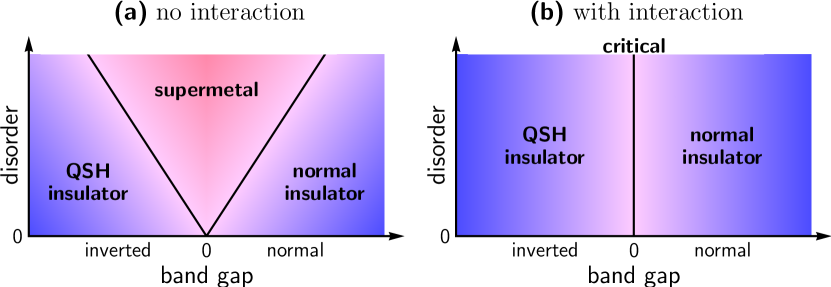
Figure 2: The phase diagrams of a disordered 2D system demonstrating the QSH effect. Left: noninteracting case. Right: interacting case (with Coulomb interaction not screened by external gates). Interaction “kills” the supermetallic phase. As a result, the two insulating phases are separated by the critical line. Adapted from Ref. 130.

Let us now return to 2D $\mathbb{Z}_{2}$ topological insulators. The 2D disordered QSH system contains only a single flavor of particles, $N=1$. Indeed, the spin-orbit interaction breaks the spin-rotational symmetry, whereas the valleys are mixed by disorder. As a result, the supermetal phase does not survive in the presence of Coulomb interaction: at $g\gg 1$ the interaction-induced localization wins. This is analogous to the case of the surface of a 3D topological insulator discussed above.

The edge of a 2D topological insulator is protected from the full localization [122]. This means that the topological distinction between the two insulating phases (ordinary and QSH insulator) is not destroyed by the interaction, whereas the supermetallic phase separating them disappears. Therefore, the transition between two insulators occurs through an interaction-induced critical state[130], see Fig. 2 (right panel).

7 Summary

Despite its half-a-century age, Anderson localization remains a very actively developing field. In this article, we have reviewed some of recent theoretical advances in the physics of Anderson transitions, with an emphasis on manifestations of criticality and on the impact of underlying symmetries and topologies. The ongoing progress in experimental techniques allows one to explore these concepts in a variety of materials, including semiconductor structures, disordered superconductors, graphene, topological insulators, atomic systems, light and sound propagating in random media, etc.

We are very grateful to a great many of colleagues for fruitful collaboration and stimulating discussions over the years of research work in this remarkable field. The work was supported by the DFG – Center for Functional Nanostructures, by the EUROHORCS/ESF (IVG), and by Rosnauka grant 02.740.11.5072.

References

- 1. P. W. Anderson, Phys. Rev. 109, 1492 (1958).
- 2. P. A. Lee and T. V. Ramakrishnan, Rev. Mod. Phys. 57, 287 (1985).
- 3. B. Kramer and A. MacKinnon, Rep. Prog. Phys. 56, 1469 (1993).
- 4. B. Huckestein, Rev. Mod. Phys. 67, 357 (1995).
- 5. K. B. Efetov, Adv. Phys. 32, 53 (1983); Supersymmetry in Disorder and Chaos (Cambridge University Press, 1997).
- 6. F. Evers and A. D. Mirlin, Rev. Mod. Phys. 80, 1355 (2008).
- 7. A. Altland and M. R. Zirnbauer, Phys. Rev. B 55, 1142 (1997).
- 8. M. R. Zirnbauer, J. Math. Phys. 37, 4986 (1996); P. Heinzner, A. Huckleberry, and M. R. Zirnbauer, Commun. Math. Phys. 257, 725 (2005).
- 9. A. M. M. Pruisken, Nucl. Phys. B 235, 277 (1984); in The Quantum Hall Effect, ed. by R.E. Prange and S.M. Girvin (Springer, 1987), p. 117.
- 10. M. Janßen, Int. J. Mod. Phys. B 8, 943 (1994).
- 11. A. D. Mirlin, Y. V. Fyodorov, F.-M. Dittes, J. Quezada, and T. H. Seligman, Phys. Rev. E 54, 3221 (1996).
- 12. A. D. Mirlin, Phys. Rep. 326, 259 (2000).
- 13. F. Evers and A. D. Mirlin, Phys. Rev. Lett. 84, 3690 (2000); A. D. Mirlin and F. Evers, Phys. Rev. B 62, 7920 (2000).
- 14. D. Thouless, Phys. Rep. 13, 93 (1974).
- 15. F. Wegner, Z. Phys. B 25, 327 (1996).
- 16. E. Abrahams, P. W. Anderson, D. C. Licciardello, and T. V. Ramakrishnan, Phys. Rev. Lett. 42, 673 (1979).
- 17. F. Wegner, Z. Phys. B 35, 207 (1979).
- 18. L. P. Gor’kov, A. I. Larkin, and D. Khmel’nitskii, JETP Lett. 30, 248 (1979).
- 19. D. Vollhardt and P. Wölfle, Phys. Rev. B 22, 4666 (1980).
- 20. L. Schaefer and F. Wegner, Z. Phys. B 38, 113 (1980).
- 21. K. Jüngling and R. Oppermann, Z. Phys. B 38, 93 (1980).
- 22. K. B. Efetov, A. I. Larkin, and D. E. Khmeniskii, Sov. Phys. JETP 52, 568 (1980).
- 23. P. Wölfle and R. N. Bhatt, Phys. Rev. B 30, 3542 (1984).
- 24. T. Guhr, A. Müller-Gröling, and H. A. Weidenmüller, Phys. Rep. 299, 189 (1998).
- 25. M. R. Zirnbauer, math-ph/0404057 (2004).
- 26. S. Hikami, Phys. Lett. 98B, 208 (1981)
- 27. F. Wegner, Nucl. Phys. B 316, 663 (1989).
- 28. M. Schreiber and H. Grussbach, Phys. Rev. Lett. 76, 1687 (1996).
- 29. F. Wegner, Z. Physik B 36, 209 (1980).
- 30. C. Castellani and L. Peliti, J. Phys. A: Math. Gen. 19, L429 (1986).
- 31. B. B. Mandelbrot, J. Fluid Mech. 62, 331 (1974).
- 32. J.T. Chalker, Physca A 167, 253 (1990).
- 33. F. Wegner, in Localisation and Metal Insulator transitions, ed. by H. Fritzsche and D. Adler (Plenum, N.Y. 1985), 337.
- 34. B. Duplantier and A. W. W. Ludwig, Phys. Rev. Lett. 66, 247 (1991).
- 35. C. Mudry, C. Chamon, and X.-G. Wen, Nucl. Phys. B 466, 383 (1996).
- 36. T. C. Halsey, M. H. Jensen, L. P. Kadanoff, I. Procaccia, and B. I. Shraiman, Phys. Rev. A 33, 1141 (1986).
- 37. A. D. Mirlin, Y. V. Fyodorov, A. Mildenberger, and F. Evers, Phys. Rev. Lett. 97, 046803 (2006).
- 38. A. Mildenberger, A. R. Subramaniam, R. Narayanan, F. Evers, I. A. Gruzberg, and A. D. Mirlin, Phys. Rev. B 75, 094204 (2007).
- 39. A. Mildenberger and F. Evers, Phys. Rev. B 75, 041303(R) (2007).
- 40. H. Obuse, A. R. Subramaniam, A. Furusaki, I. A. Gruzberg, and A. Ludwig, Phys. Rev. Lett. 98, 156802 (2007).
- 41. A. Mildenberger, F. Evers, and A. D. Mirlin, Phys. Rev. B 66, 033109 (2002).
- 42. F. Wegner, Nucl. Phys. B 280, 210 (1987).
- 43. A. R. Subramaniam, I. A. Gruzberg, A. W. W. Ludwig, F. Evers, A. Mildenberger, and A. D. Mirlin, Phys. Rev. Lett. 96, 126802 (2006).
- 44. M. Morgenstern, J. Klijn, Chr. Meyer, and R. Wiesendanger, Phys. Rev. Lett. 90, 056804 (2003); K. Hashimoto, C. Sohrmann, J. Wiebe, T. Inaoka, F. Meier, Y. Hirayama, R.A. Römer, R. Wiesendanger, and M. Morgenstern, Phys. Rev. Lett. 101, 256802 (2008).
- 45. J. Chabé, G. Lemarié, B. Grémaud, D. Delande, P. Szriftgiser, and J.C. Garreau, Phys. Rev. Lett. 101, 255702 (2008).
- 46. H. Hu, A. Strybulevych, J.H. Page, S.E. Skipetrov, and B.A. van Tiggelen, Nature Phys. 4, 945 (2008).
- 47. S. Faez, A. Strybulevych, J. H. Page, Ad Lagendijk, and B.A. van Tiggelen, Phys. Rev. Lett. 103, 155703 (2009).
- 48. A. Richardella, P. Roushan, S. Mack, B. Zhou, D.A. Huse, D.D. Awschalom, and A. Yazdani, Science 327, 665 (2010).
- 49. M.V. Feigel’man, L.B. Ioffe, V.E. Kravtsov, and E. Cuevas, arXiv:1002.0859.
- 50. R. Abou-Chacra, P. W. Anderson, and D. J. Thouless, J. Phys. C 6, 1734 (1973).
- 51. K. B. Efetov, Sov. Phys. JETP 61, 606 (1985); ibid 65, 360 (1987).
- 52. M. R. Zirnbauer, Phys. Rev. B 34, 6394 (1986); Nucl. Phys. B 265, 375 (1986).
- 53. A. D. Mirlin and Y. V. Fyodorov, Nucl. Phys. B 366, 507 (1991).
- 54. K. B. Efetov, Physica A 167, 119 (1990).
- 55. Y. V. Fyodorov, A. D. Mirlin, and H.-J. Sommers, J. Phys. I France 2, 1571 (1992).
- 56. A. D. Mirlin and Y. V. Fyodorov, Phys. Rev. Lett. 72, 526; J. Phys. I France 4, 655.
- 57. E.P. Wigner, Ann. Math. 53, 36 (1951).
- 58. F.J. Dyson, J. Math. Phys. 3, 140, 1199 (1962).
- 59. S. Helgason, Differential Geometry, Lie Groups, and Symmetric Spaces (Academic Press, New York, 1978).
- 60. M. Caselle and U. Magnea, Phys. Rep. 394, 41 (2004).
- 61. P. Fendley, in New Theoretical Approaches to Strongly Correlated Systems (Cambridge, 2000).
- 62. R. Gade, Nucl. Phys. B 398, 499 (1993).
- 63. R. Gade and F. Wegner, Nucl. Phys. B 360, 213 (1991).
- 64. K. Slevin and T. Nagao, Phys. Rev. Lett. 70, 635 (1993).
- 65. J. J. M. Verbaarschot and I. Zahed, Phys. Rev. Lett. 70, 3852.
- 66. V. Kagalovsky, B. Horovitz, Y. Avishai, and J.T. Chalker, Phys. Rev. Lett. 82, 3516 (1999).
- 67. I.A. Gruzberg, A.W.W. Ludwig, and N. Read, Phys. Rev. Lett. 82, 4524 (1999).
- 68. T. Senthil, J.B. Marston, and M.P.A. Fisher, Phys. Rev. B 60, 4245 (1999).
- 69. E.J. Beamond, J. Cardy, and J.T. Chalker, Phys. Rev. B 65, 214301 (2002).
- 70. F. Evers, A. Mildenberger, and A.D. Mirlin, Phys. Rev. B 67, 041303(R) (2003); A.D. Mirlin, F. Evers, and A. Mildenberger, J. Phys. A: Math. Gen. 36, 3255 (2003).
- 71. S. Cho and M.P.A. Fisher, Phys. Rev. B, 55, 1025 (1997).
- 72. T. Senthil and M.P.A. Fisher, Phys. Rev. B 61, 6966 (2000)
- 73. J. T. Chalker, N. Read, V. Kagalovsky, B. Horovitz, Y. Avishai, and A. W. W. Ludwig, Phys. Rev. B 65, 012506 (2002).
- 74. A. Mildenberger, F. Evers, A.D. Mirlin, and J.T. Chalker, Phys. Rev. B 75, 245321 (2007).
- 75. D. A. Ivanov, Vortices in Unconventional Superconductors and Superfluids, edited by R. P. Huebener, N. Schopol, and G. E. Volovik (2002), p. 253; J. Math. Phys. 43, 126 (2002).
- 76. E. Witten, Commun. Math. Phys. 92, 455 (1984).
- 77. A. A. Nersesyan, A. M. Tsvelik, and F. Wenger, Phys. Rev. Lett. 72, 2628 (1994); Nucl. Phys. B 438, 561 (1995).
- 78. A. Altland, B.D. Simons, and M.R. Zirnbauer, Phys. Rep. 359, 283 (2002).
- 79. M. Bocquet, D. Serban, and M.R. Zirnbauer, Nucl. Phys. B 578, 628 (2000).
- 80. V.S. Dotsenko and V.S. Dotsenko, Adv. Phys. 32, 129 (1983).
- 81. S. Guruswamy, A. LeClair, and A.W.W. Ludwig, Nucl. Phys. B 583, 475 (2000).
- 82. E. McCann, K. Kechedzhi, V.I. Fal’ko, H. Suzuura, T. Ando, and B.L. Altshuler, Phys. Rev. Lett. 97, 146805 (2006);
- 83. A.W.W. Ludwig, M.P.A. Fisher, R. Shankar, and G. Grinstein, Phys. Rev. B 50, 7526 (1994)
- 84. D. V. Khveshchenko, Phys. Rev. Lett. 97, 036802 (2006).
- 85. I.L. Aleiner and K.B. Efetov, Phys. Rev. Lett. 97, 236801 (2006).
- 86. A. Altland, Phys. Rev. Lett. 97, 236802 (2006).
- 87. P.M. Ostrovsky, I.V. Gornyi, and A.D. Mirlin, Phys. Rev B 74, 235443 (2006).
- 88. P.M. Ostrovsky, I.V. Gornyi, and A.D. Mirlin, Phys. Rev. Lett. 98, 256801 (2007)
- 89. P.M. Ostrovsky, I.V. Gornyi, and A.D. Mirlin, Eur. Phys. J. Special Topics 148, 63 (2007)
- 90. D. Bernard and A. LeClair, J. Phys A 35, 2555 (2002).
- 91. A.K. Geim and K.S. Novoselov, Nature Materials 6, 183 (2007).
- 92. A.H. Castro Neto, F. Guinea, N.M.R. Peres, K.S. Novoselov, and A.K. Geim, Rev. Mod. Phys. 81, 109 (2009).
- 93. K.S. Novoselov, A.K. Geim, S.V. Morozov, D. Jiang, M.I. Katsnelson, I.V. Grigorieva, S.V. Dubonos, and A.A. Firsov, Nature (London) 438, 197 (2005).
- 94. Y. Zhang, Y.-W. Tan, H.L. Stormer, and P. Kim, Nature (London) 438, 201 (2005).
- 95. Y.-W. Tan, Y. Zhang, H.L. Stormer, and P. Kim, Eur. Phys. J. Special Topics, 148, 15 (2007).
- 96. J. H. Bardarson et al., Phys. Rev. Lett. 99, 106801 (2007); K. Nomura et al., ibid. 99, 146806 (2007).
- 97. J.-S. Caux, Phys. Rev. Lett. 81, 4196 (1998); J.-S. Caux, N. Taniguchi, and A.M. Tsvelik, Nucl. Phys. B 525, 621 (1998).
- 98. A.M. Tsvelik, Phys. Rev. B 51, 9449 (1995).
- 99. J. Schwinger, Phys. Rev. 128, 2425 (1962).
- 100. S. Ryu, C. Mudry, A. Furusaki, and A.W.W. Ludwig, Phys. Rev. B 75, 205344 (2007).
- 101. B. L. Altshuler and A. G. Aronov, in Electron-electron interactions in disordered conductors, edited by A. L. Efros and M. Pollak (Elsevier, 1985), p. 1.
- 102. A. M. Finkelstein, Sov. Sci. Rev. A. Phys. 14, 1 (1990).
- 103. D. Belitz and T. R. Kirkpatrick, Rev. Mod. Phys. 66, 261 (1994).
- 104. E. Abrahams, S.V. Kravchenko, and M.P. Sarachik, Rev. Mod. Phys. 73, 251 (2001).
- 105. A. Punnoose and A. M. Finkel’stein, Phys. Rev. Lett. 88, 016802 (2001); Science 310, 289 (2005).
- 106. T. Giamarchi and H. Schulz, Phys. Rev. B 37, 325 (1988).
- 107. T. Giamarchi, Quantum Physics in One Dimension (Oxford University Press, 2004).
- 108. L. Fleishman, D.C. Licciardello, and P.W. Anderson, Phys. Rev. Lett. 40, 1340 (1978).
- 109. L. Fleishman and P.W. Anderson, Phys. Rev. B 21, 2366 (1980).
- 110. I.V. Gornyi, A.D. Mirlin, and D.G. Polyakov, Phys. Rev. Lett. 95, 206603 (2005)
- 111. D.M. Basko, I.L. Aleiner, and B.L. Altshuler, Ann. Phys. (N.Y.) 321, 1126 (2006).
- 112. B.L. Altshuler, Y. Gefen, A. Kamenev, and L.S. Levitov, Phys. Rev. Lett. 78, 2803 (1997).
- 113. S.-Y. Hsu and J.M. Valles, Jr., Phys. Rev. Lett. 74, 2331 (1995).
- 114. F.W. Van Keuls, H. Mathur, H.W. Jiang, and A.J. Dahm, Phys. Rev. B 56, 13263 (1997).
- 115. Y.B. Khavin, M.E. Gershenson, and A.L. Bogdanov, Phys. Rev. B 58, 8009 (1998).
- 116. G.M. Minkov, A.V. Germanenko, O.E. Rut, A.A. Sherstobitov, and B.N. Zvonkov, Phys. Rev. B 75, 235316 (2007).
- 117. V. Oganesyan and D.A. Huse, Phys. Rev. B 75, 155111 (2007).
- 118. D.A. Knyazev, O.E. Omel’yanovskii, V.M. Pudalov, I.S. Burmistrov, Phys. Rev. Lett. 100, 046405 (2008).
- 119. A. Punnoose, A. M. Finkel’stein, A. Mokashi, S. V. Kravchenko, arXiv:0910.5510
- 120. I.V. Gornyi, A.D. Mirlin, and D.G. Polyakov, Phys. Rev. B 75, 085421 (2007).
- 121. C. Monthus and T. Garel, arXiv:1001.2984
- 122. C. L. Kane and E. J. Mele, Phys. Rev. Lett. 95, 146802 (2005); ibid. 95, 226801 (2005).
- 123. B. A. Bernevig et al., Science 314, 1757 (2006); B. A. Bernevig and S.-C. Zhang, Phys. Rev. Lett. 96, 106802 (2006).
- 124. X.-L. Qi et al., Phys. Rev. B 78, 195424 (2008).
- 125. M. König et al., Science 318, 766 (2007).
- 126. D. Hsieh et al., Nature 452, 970 (2008).
- 127. M. König et al., J. Phys. Soc. Jpn. 77, 031007 (2008); A. Roth et al., Science 325, 294 (2009).
- 128. D. Hsieh et al., Science 323, 919 (2008); P. Roushan et al., Nature 460, 1106 (2009).
- 129. D. Hsieh et al., Nature 460, 1101 (2009); Y. L. Chen et al., Science 325, 178 (2009); Y. Xia et al., Nature Phys. 5, 398 (2009); H. Zhang et al., ibid. 5, 438 (2009).
- 130. P.M. Ostrovsky, I.V. Gornyi, and A.D. Mirlin, arXiv:0910.1338.
- 131. L. Sheng et al., Phys. Rev. Lett. 95, 136602 (2005).
- 132. G. E. Volovik, JETP 67, 1804 (1988); G. E. Volovik and V. M. Yakovenko, J. Phys.: Condens. Matter 1, 5263 (1989).
- 133. L. Fu et al., Phys. Rev. Lett. 98, 106803 (2007); L. Fu and C. L. Kane, Phys. Rev. B 76, 045302 (2007).
- 134. A. P. Schnyder et al., Phys. Rev. B 78, 195125 (2008); AIP Conf. Proc. 1134, 10 (2009); S.Ryu et al., arXiv:0912.2157.
- 135. A. Yu. Kitaev, AIP Conf. Proc. 1134, 22 (2009).
- 136. M. Onoda et al., Phys. Rev. Lett. 98, 076802 (2007); S. Murakami et al., Phys. Rev. B 76, 205304 (2007).
- 137. H. Obuse et al., Phys. Rev. B 76, 075301 (2007); S.Ryu et al., arXiv:0912.2158.
- 138. M.I. D’yakonov and A.V. Khaetskii, JETP Lett. 33, 110 (1981).
- 139. V.A. Volkov and T.N. Pinsker. Sov. Phys. Solid State 23, 1022 (1981); B.A. Volkov and O.A. Pankratov, JETP Lett. 42, 178 (1985).
- 140. S.-S. Lee and S. Ryu, Phys. Rev. Lett. 100, 186807 (2008).
- 141. A. M. M. Pruisken and I. S. Burmistrov, Ann. Phys. (N.Y.) 322, 1265 (2007).