On the initial-value problem of the Maxwell-Lorentz equations

Abstract

We consider the Maxwell-Lorentz equations, i.e., the equation of motion of a charged dust coupled to Maxwell’s equations, on an arbitrary general-relativistic spacetime. We decompose this system of equations into evolution equations and constraints, and we demonstrate that the evolution equations are strongly hyperbolic. This result guarantees that the initial-value problem of the Maxwell-Lorentz equations is well-posed. We illustrate this general result with a discussion of spherically symmetric solutions on Minkowski spacetime.

1 Introduction

In this article we consider the equations of motion for a charged dust coupled to an electromagnetic field on a general-relativistic spacetime. These equations of motion are often refered to as the Maxwell-Lorentz equations, because they comprise the Maxwell equations for the electromagnetic field and the Lorentz force equation for the dust particles. Here, as usual, we use the word “dust” as synonymous to “pressure-less fluid”. As an alternative, the name “cold fluid” is sometimes used.

The Maxwell-Lorentz equations have several interesting applications. E.g., they can be used for describing the electron component in a plasma. Among other things, this is of relevance for astrophysics, e.g., for modeling the Solar corona. In spite of the high temperature of the Solar corona, it is quite reasonable to model the electron component as a pressure-less (or “cold”) fluid, because the density is low. The Maxwell-Lorentz equations have also been suggested for modeling a beam of charged particles in an accelerator, cf. Burton, Gratus and Tucker [1]. Special interest has been given to the Maxwell-Lorentz equations for rigid charge distributions on Minkowski spacetime. The idea is to use this as a model for an extended charged classical particle, with the self-interaction taken into account. Interesting results have been found, e.g., by Spohn and collaborators [2, 3, 4] as well as by Bauer and Dürr [5]. An important goal of this line of research is to get some new insight into the point-particle limit and its notorious pathologies.

Several fundamental features of the Maxwell-Lorentz equations on Minkowski spacetime are discussed in Chapter 5 of Parrott’s text-book on electrodynamics [6]. Among other things, Parrott discusses the initial-value problem for these equations. Using the Cauchy-Kowalevski theorem, he is able to demonstrate local existence and uniqueness of (analytic) solutions from analytic initial data. However, the assumption of analyticity is physically not quite satisfactory: Knowing an analytic function on an arbitrarily small neighborhood fixes the function on the whole domain of convergence of the Taylor series, whereas physical measurements in an arbitrarily small neighborhood cannot determine any results outside of the causal future of this neighborhood. Also, it is often convenient to consider fields which are zero on an open subset $\mathcal{U}$ and non-zero on the complement of $\overline{\mathcal{U}}$; such fields cannot be analytic near the boundary of $\mathcal{U}$. For these reasons it is desirable to have an existence and uniqueness theorem for non-analytic data, as noted by Parrott himself. It is the main purpose of this paper to establish such a result.

To that end we decompose the Maxwell-Lorentz equations, on an arbitrary general-relativistic spacetime, into evolution equations and constraints. The evolution equations can be written as a quasi-linear system of first order partial differential equations. We derive the characteristic equation (dispersion relation), and we demonstrate that the system of evolution equations is strongly hyperbolic, which is a necessary and sufficient condition for the initial-value problem to be well-posed. This means that a solution locally exists, that it is unique, and that it depends continuously on the data in an appropriate topology. This result is of relevance for solving the Maxwell-Lorentz equations numerically: If a solution does not exist it is pointless to write a numerical code that tries to approximate it; if the solution is not unique the code does not know which solution to approximate; and if the dependence on the data is discontinuous it is impossible to estimate the error of a numerical solution.

After establishing our general existence and uniqueness result, we illustrate it with a discussion of spherically symmetric solutions on Minkowski spacetime.

2 The Maxwell-Lorentz equations

We consider the coupled equations of motion of a charged dust and an electromagnetic field on a general-relativistic spacetime, i.e., on a 4-dimensional manifold $M$ with a Lorentzian metric $g$. We allow for an external electric current density $J^{e}$, and we assume that the dust consists of only one species of particles, with charge $q$ and mass $m$. In the following we assume that the second-rank tensor field $g=g_{ij}dx^{i}\otimes dx^{j}$, the one-form $J^{e}=J_{i}^{e}dx^{i}$ and the constants $q$ and $m$ are given. We use standard index notation with Einstein’s summation convention for latin indices taking values $0,1,2,3$ and for greek indices taking values $1,2,3$. As usual, the contravariant metric components are defined by $g^{ki}g{}_{ij}=\delta^{k}_{j}$. The metric has signature $(-,+,+,+)$ and its Levi-Civita connection is denoted $\nabla$. We use units making $\varepsilon_{0}$ and $\mu_{0}$ (and, thus, the vacuum speed of light $c$) equal to 1.

The equations of motion consist of Maxwell’s equations for the electromagnetic field and the Lorentz force equation for the dust particles,

$$\partial_{i}F_{jk}\,+\,\partial_{j}F_{ki}\,+\,\partial_{k}F_{ij}\,=\,0\;,$$ (1)

$$g^{ij}\nabla_{i}F_{jk}\,=\,\,J_{k}^{e}\,-\,q\,n\,g_{k\ell}U^{\ell}\;,$$ (2)

$$U^{i}\nabla_{i}U^{j}\,=\,\dfrac{q}{m}\,g^{jk}F_{k\ell}U^{\ell}\;.$$ (3)

We refer to these equations as to the Maxwell-Lorentz equations. The field variables (i.e., the “unknowns” in these equations) are

• the electromagnetic field strength $F_{ij}dx^{i}\otimes dx^{j}$ which is an antisymmetric second-rank tensor field, $F_{ij}=-F_{ji}\,$;

• the four-velocity $U^{i}\partial_{i}$ of the dust which is a vector field, normalised to $g_{ij}U^{i}U^{j}=-1\,$.

• the (proper) number density $n$ of the dust which is a non-negative scalar function;

The electromagnetic field is to be interpreted as the field produced by the external current plus the field produced by the charged dust plus, possibly, an additional source-free field.

If $n=0$ on an open subset of the spacetime, $U^{i}$ is physically undetermined on this subset. In this case, the electromagnetic field is determined by (1) and (2), i.e., by Maxwell’s equations with a given source $J_{k}^{e}$. As the initial-value problem for this system of equations is well-known, we assume in the following that $n>0$ on our spacetime manifold. (Or, to put this another way, we restrict our spacetime to an open subset on which $n>0$.)

Note that (3) implies $U^{i}\partial_{i}\big{(}g_{jk}U^{j}U^{k}\big{)}=0$. This guarantees that, if the condition $g_{jk}U^{j}U^{k}=-1$ is satisfied at one point, then it is satisfied along the whole integral curve of $U^{i}\partial_{i}$ that passes through this point. A similar statement is true for the condition $n>0$, provided that the external current is conserved, $g^{ik}\nabla_{i}J_{k}^{e}=0$. To prove this, we read from (2) that the conservation law for the external current implies $\nabla_{k}\big{(}nU^{k}\big{)}=0$ and thus

$$U^{k}\partial_{k}n+n\nabla_{k}U^{k}=0\;.$$ (4)

If $x(t)$ is an integral curve of the vector field $U^{i}\partial_{i}$, integration of (4) yields

$$n\big{(}x(t_{2})\big{)}\,=\,n\big{(}x(t_{1})\big{)}\,\mathrm{exp}\Big{\{}-\int_{t_{1}}^{t_{2}}\big{(}\nabla_{k}U^{k}\big{)}\big{(}x(t)\big{)}\,dt\Big{\}}$$ (5)

so $n$ cannot change sign along an integral curve of $U^{i}\partial_{i}$. This is an important observation in view of the initial value problem. It makes sure that, for a solution of the Maxwell-Lorentz equations, it suffices to check the conditions $g_{ij}U^{i}U^{j}=-1$ and $n>0$ on the initial hypersurface.

To illustrate the physical content of the Maxwell-Lorentz equations we briefly mention two different applications. Firstly, we can use these equations for modeling plasma waves in the Solar corona. In this case we would choose for $(M,g)$ the Schwarzschild spacetime, for $J^{e}$ the electric current density of the ion component which could be assumed static, and for $q$ and $m$ the charge and the mass of the electron. The field variables are the total electromagnetic field, the four-velocity of the electrons and the number density of the electrons. Secondly, we can consider an electron beam in an accelerator. Then we would choose for $(M,g)$ an open subset of the Minkowski spacetime (to model the spacetime region inside the accelerator pipe), for $J^{e}$ the zero one-form (as there is no external current inside the accelerator pipe), and for $q$ and $m$ the charge and the mass of the electron. The field variables are again the total electromagnetic field (i.e., the field produced by the dust and the accelerating field which has no sources inside the pipe), the four-velocity of the electrons and the number density of the electrons.

3 Decomposition of the Maxwell-Lorentz equations into evolution equations and constraints

We fix a spacetime point $P$ and we choose local coordinates, on an appropriate neighborhood of $P$, such that the hypersurfaces $x^{0}=\,$constant are spacelike and the $x^{0}-$lines are perpendicular to these hypersurfaces. We want to discuss if the prescription of appropriate initial data on the hypersurface $x^{0}=\,$constant through $P$ determines a unique solution of the Maxwell-Lorentz equations on some neighborhood of $P$. To that end we have to decompose the Maxwell-Lorentz equations into evolution equations (i.e., equations that do contain $\partial_{0}$ derivatives) and constraints (i.e., equations that do not contain $\partial_{0}$ derivatives).

There are two constraints, given by equation (1) with all three indices spatial and by equation (2) with $k=0$. After expressing covariant derivatives in terms of partial derivatives, introducing the Christoffel symbols of the metric tensor, these two equations take the following form.

$$\partial_{\mu}F_{\nu\sigma}\,+\,\partial_{\nu}F_{\sigma\mu}\,+\,\partial_{\sigma}F_{\mu\nu}\,=\,0\;,$$ (6)

$$g^{\mu\nu}\big{(}\partial_{\mu}F_{\nu 0}-\Gamma_{\mu\nu}^{\sigma}F_{\sigma 0}-\Gamma_{\mu 0}^{\sigma}F_{\nu\sigma}-\Gamma_{\mu 0}^{0}F_{\nu 0}\big{)}\,=\,J_{0}^{e}\,-\,q\,n\,g_{00}U^{0}\;.$$ (7)

The remaining equations are the evolution equations: Evaluating equation (1) with one of the indices equal to 0 gives three scalar equations,

$$\partial_{0}F_{\mu\nu}\,+\,\partial_{\mu}F_{\nu 0}\,+\,\partial_{\nu}F_{0\mu}\,=\,0\;.$$ (8)

Evaluating equation (2) with a spatial index, $k=\sigma$, gives another three scalar equations. After eliminating the number density $n$, with the help of (7), these equations read

$$\partial_{0}F_{0\sigma}\,+\,\dfrac{g^{\mu\nu}}{g^{00}}\,\partial_{\mu}F_{\nu\sigma}\,-\,\dfrac{U^{\rho}}{U^{0}}\,g_{\sigma\rho}g^{\mu\nu}\partial_{\mu}F_{\nu 0}\,=\,\dfrac{g^{\mu\nu}}{g^{00}}\,\big{(}\Gamma_{\mu\nu}^{0}F_{0\sigma}+\Gamma_{\mu\nu}^{\rho}F_{\rho\sigma}+\Gamma_{\mu\sigma}^{0}F_{\nu 0}+\Gamma_{\mu\sigma}^{\rho}F_{\nu\rho}\big{)}$$

$$\,-\,\dfrac{U^{\rho}}{U^{0}}\,g_{\sigma\rho}g^{\mu\nu}\big{(}\Gamma_{\mu\nu}^{\tau}F_{\tau 0}+\Gamma_{\mu 0}^{\rho}F_{\nu\rho}+\Gamma_{\mu 0}^{0}F_{\nu 0}\big{)}\,+\,\Gamma_{00}^{0}F_{0\sigma}\,+\,\Gamma_{00}^{\mu}F_{\mu\sigma}\,+\,\Gamma_{0\sigma}^{\mu}F_{0\mu}\,+\,\dfrac{J_{\sigma}^{e}}{g^{00}}\,-\,\dfrac{U^{\rho}}{U^{0}}\,g_{\sigma\rho}\,J_{0}^{e}\;.$$ (9)

Finally, evaluating equation (3) with a spatial index, $j=\sigma$, gives us again three scalar equations. With the help of equation (3) with $j=0$, these equations can be rewritten as

$$\partial_{0}\dfrac{U^{\sigma}}{U^{0}}\,+\,\dfrac{U^{\rho}}{U^{0}}\partial_{\rho}\dfrac{U^{\sigma}}{U^{0}}\,=\,-\,\Gamma_{00}^{\sigma}\,-\,2\Gamma_{0\mu}^{\sigma}\,\dfrac{U^{\mu}}{U^{0}}\,-\,\Gamma_{\mu\nu}^{\sigma}\,\dfrac{U^{\mu}U^{\nu}}{(U^{0})^{2}}$$

$$+\,\dfrac{q}{m}\,\dfrac{1}{U^{0}}\,\Big{\{}g^{\sigma\tau}\Big{(}\,F_{\tau 0}\,+\,F_{\tau\rho}\,\dfrac{U^{\rho}}{U^{0}}\,\Big{)}\,-\,\dfrac{U^{\sigma}U^{\tau}}{(U^{0})^{2}}\,g^{00}\,F_{0\tau}\,\Big{\}}\,\;.$$ (10)

Equation (3) with $j=0$ can be ignored because it is automatically satisfied if the other equations are, owing to the normalisation condition $g_{ij}U^{i}U^{j}=-1\,$. So the system of evolution equations is given by nine scalar equations, (8), (9) and (10). Note that the number density $n$ is not a dynamical variable; $n$ has been eliminated from the evolution equations and is algebraically determined by the other field variables via (7).

To write the evolution equations in a more convenient form, we decompose the electromagnetic field into its electric and magnetic components, $E_{\sigma}$ and $B^{\nu}$, with respect to the chosen coordinate system,

$$F_{\sigma 0}\,=\,E_{\sigma}\qquad\mathrm{and}\qquad F_{\tau\rho}\,=\,\varepsilon_{\tau\rho\nu}B^{\nu}\;.$$ (11)

Here $\varepsilon_{\sigma\rho\nu}$ is the three-dimensional covariant $\varepsilon$–symbol, defined by being totally antisymmetric and satisfying $\varepsilon_{123}=1$. Moreover, we introduce the 3-velocity $v^{\sigma}$ of the dust,

$$U^{i}\partial_{i}\,=\,U^{0}\,\big{(}\partial_{0}+v^{\sigma}\partial_{\sigma}\big{)}\;,$$ (12)

Note that then $U^{0}$ is determined by the normalisation condition $(U^{0})^{2}(g_{00}+v^{\mu}v^{\nu}g_{\mu\nu})=-1\,$. If we use the three-dimensional contravariant $\varepsilon$–symbol $\varepsilon^{\sigma\rho\nu}$, defined by being totally antisymmetric and satisfying $\varepsilon^{123}=1$, we can write the evolution equations in the following final form. (We use the identity $\varepsilon^{\mu\nu\sigma}\varepsilon_{\mu\nu\tau}=2\delta^{\sigma}_{\tau}$.)

$$\partial_{0}B^{\sigma}+\varepsilon^{\sigma\mu\nu}\partial_{\mu}E_{\nu}\,=\,0\;,$$ (13)

$$\partial_{0}E_{\sigma}\,-\,\dfrac{g^{\mu\nu}}{g^{00}}\,\varepsilon_{\nu\sigma\tau}\partial_{\mu}B^{\tau}\,+\,v^{\rho}\,g_{\sigma\rho}g^{\mu\nu}\partial_{\mu}E_{\nu}\,=\,\dfrac{g^{\mu\nu}}{g^{00}}\,\big{(}\Gamma_{\mu\nu}^{0}E_{\sigma}-\Gamma_{\mu\nu}^{\rho}\varepsilon_{\rho\sigma\nu}B^{\nu}-\Gamma_{\mu\sigma}^{0}E_{\nu}-\Gamma_{\mu\sigma}^{\rho}\varepsilon_{\nu\rho\tau}B^{\tau}\big{)}$$

$$+\,v^{\rho}\,g_{\sigma\rho}g^{\mu\nu}\big{(}\Gamma_{\mu\nu}^{\tau}E_{\tau}+\Gamma_{\mu 0}^{\rho}\varepsilon_{\nu\rho\lambda}B^{\lambda}+\Gamma_{\mu 0}^{0}E_{\nu}\big{)}\,-\,\dfrac{J_{\sigma}^{e}}{g^{00}}\,+\,v^{\rho}\,g_{\sigma\rho}\,J_{0}^{e}\,+\,\Gamma_{00}^{0}E_{\sigma}\,-\,\Gamma_{00}^{\mu}\varepsilon_{\mu\sigma\nu}B^{\nu}\,+\,\Gamma_{0\sigma}^{\mu}E_{\mu}\;,$$ (14)

$$\partial_{0}v^{\sigma}\,+\,v^{\rho}\partial_{\rho}v^{\sigma}\,=\,-\,\Gamma_{00}^{\sigma}\,-\,2\Gamma_{0\mu}^{\sigma}\,v^{\mu}\,-\,\Gamma_{\mu\nu}^{\sigma}\,v^{\mu}v^{\nu}$$

$$+\,\dfrac{q}{m}\,\sqrt{-g_{00}-v^{\mu}v^{\nu}g_{\mu\nu}}\,\Big{\{}g^{\sigma\tau}\Big{(}\,E_{\tau}\,+\,\varepsilon_{\tau\rho\lambda}v^{\rho}B^{\lambda}\,\Big{)}\,+\,g^{00}v^{\sigma}v^{\tau}E_{\tau}\,\Big{\}}\;.$$ (15)

With the same notation, the constraints (6) and (7) read

$$\partial_{\mu}B^{\mu}\,=\,0\;,$$ (16)

$$q\,n\,=\,\dfrac{\sqrt{-g_{00}-v^{\lambda}v^{\rho}g_{\lambda\rho}}}{-\,g_{00}}\,\Big{(}g^{\mu\nu}\big{(}\partial_{\mu}E_{\nu}-\Gamma_{\mu\nu}^{\sigma}E_{\sigma}-\Gamma_{\mu 0}^{\sigma}\,\varepsilon_{\nu\sigma\tau}B^{\tau}-\Gamma_{\nu 0}^{0}E_{\mu}\big{)}-J_{0}^{e}\,\Big{)}\;.$$ (17)

Note that (13) implies $\partial_{0}\partial_{\sigma}B^{\sigma}=0$. Hence a solution of the evolution equations satisfies (16) everywhere if it satisfies (16) on the initial hypersurface $x^{0}=\;$constant. As a consequence, the solutions to the Maxwell-Lorentz equations can be found by solving the initial-value problem of the evolution equations, with initial values for $E_{\sigma}$, $B^{\mu}$ and $v^{\rho}$ that satisfy (16) and that give a non-negative number density $n$ via (17). Recall that, by (5), it suffices to check the condition of $n$ being positive on the initial hypersurface.

If we write

$$\vec{E}\,=\,\begin{pmatrix}E_{1}\\ E_{2}\\ E_{3}\end{pmatrix}\>,\qquad\vec{B}\,=\,\begin{pmatrix}B^{1}\\ B^{2}\\ B^{3}\end{pmatrix}\>,\qquad\vec{v}\,=\,\begin{pmatrix}v^{1}\\ v^{2}\\ v^{3}\end{pmatrix}\>,$$ (18)

the evolution equations (13), (14) and (15) can be written in matrix form as a differential equation for a 9-component column vector,

$$\partial_{0}\,\begin{pmatrix}\vec{E}\\ \vec{B}\\ \vec{v}\end{pmatrix}\,-\,\boldsymbol{L}^{\rho}\partial_{\rho}\begin{pmatrix}\vec{E}\\ \vec{B}\\ \vec{v}\end{pmatrix}\,=\,\begin{pmatrix}\vec{m}{}_{1}\\ \vec{m}{}_{2}\\ \vec{m}{}_{3}\end{pmatrix}\;.$$ (19)

Here, $\boldsymbol{L}^{1},\boldsymbol{L}^{2},\boldsymbol{L}^{3}$ are $9\times 9$ matrices and $\vec{m}{}_{1}$, $\vec{m}{}_{2}$, $\vec{m}{}_{3}$ are 3-component column vectors. All of them depend on the spacetime coordinates, via the given background fields. In addition, the $\boldsymbol{L}^{\rho}$ depend on $\vec{v}$ and the $\vec{m}{}_{\rho}$ depend on all dynamical variables $(\vec{E},\vec{B},\vec{v})$, but not on their derivatives. Hence, (19) is a quasi-linear system of first-order differential equations for $(\vec{E},\vec{B},\vec{v})$.

We can choose our coordinates such that, at the fixed spacetime point $P$, we have $(g_{\mu\nu})=\mathrm{diag}(-1,1,1,1)$ and $\Gamma_{\mu\nu}^{\sigma}=0$. Then we can read from (13), (14) and (15) that, at this point,

$$\boldsymbol{L}^{\rho}\,=\,\begin{pmatrix}-\vec{v}\otimes\vec{e}{\,}^{\rho}&-\boldsymbol{A}^{\rho}&\boldsymbol{0}\\ \boldsymbol{A}^{\rho}&\boldsymbol{0}&\boldsymbol{0}\\ \boldsymbol{0}&\boldsymbol{0}&-v^{\rho}\,\boldsymbol{1}\\ \end{pmatrix}$$ (20)

where

$$\vec{e}{\,}^{1}\,=\,\begin{pmatrix}1\\ 0\\ 0\end{pmatrix}\;,\qquad\vec{e}{\,}^{2}\,=\,\begin{pmatrix}0\\ 1\\ 0\end{pmatrix}\;,\qquad\vec{e}{\,}^{3}\,=\,\begin{pmatrix}0\\ 0\\ 1\end{pmatrix}\;,$$ (21)

$$\boldsymbol{A}^{1}\,=\,\begin{pmatrix}0&0&0\\ 0&0&1\\ 0&-1&0\end{pmatrix}\;,\qquad\boldsymbol{A}^{2}\,=\,\begin{pmatrix}0&0&-1\\ 0&0&0\\ 1&0&0\end{pmatrix}\;,\qquad\boldsymbol{A}^{3}\,=\,\begin{pmatrix}0&1&0\\ -1&0&0\\ 0&0&0\end{pmatrix}\;.$$ (22)

The $\vec{m}{}_{\rho}$ are given, at the point $P$, by

$$\vec{m}{}_{1}\,=\,\vec{J}{}^{e}\,+\,J_{0}^{e}\vec{v}\;,\qquad\vec{m}{}_{2}\,=\,\vec{0}\;,\qquad\vec{m}{}_{3}\,=\,\dfrac{q}{m}\,\sqrt{1-v^{\tau}v^{\lambda}\delta_{\tau\lambda}}\,\big{(}\vec{E}+\varepsilon_{\mu\nu\sigma}v^{\mu}B^{\nu}\vec{e}{\,}^{\sigma}-v^{\rho}E_{\rho}\vec{v}\big{)}\;.$$ (23)

If $(M,g)$ is Minkowski spacetime, and if we use standard Minkowski coordinates, (20) and (23) hold not only at one point but everywhere.

4 Strong hyperbolicity of the Maxwell-Lorentz equations

In this section we will demonstrate that the initial-value problem for the evolution equations of the Maxwell-Lorentz system is well-posed. If we assume that the background fields are analytic, and that we give analytic initial data for $(\vec{E},\vec{B},\vec{v})$, local existence and uniqueness of a solution follows from the Cauchy-Kowalevsky theorem; this was the result found by Parrott [6]. (Parrott only considered the case that $(M,g)$ is Minkowski spacetime and that $J^{e}$ vanishes, but the result carries over immediately to our more general case.) For the reasons outlined in the introduction, we want to have an existence and uniqueness statement for non-analytic data. To that end we have to recall some terminology and some results from the theory of partial differential equations.

For a quasi-linear system of first-order partial differential equations of the form (19), the left-hand side of (19) is called the principal part. Existence and uniqueness of solutions is completely determined by the principal part and hence by the matrices $\boldsymbol{L}^{\rho}$. (19) is called hyperbolic if for any $\vec{p}=p_{\rho}\vec{e}{\,}^{\rho}\in\mathbb{R}^{3}$ the eigenvalues of the $9\times 9$ matrix $p_{\rho}\boldsymbol{L}^{\rho}$ are real. (19) is called strongly hyperbolic or symmetrisable if, in addition, for each eigenvalue the geometric multiplicity equals the algebraic multiplicity, i.e., if $p_{\rho}\boldsymbol{L}^{\rho}$ has nine linearly independent real eigenvectors. An equivalent condition is that there exists a matrix $\boldsymbol{H}(\vec{p})$ such that $\boldsymbol{H}(\vec{p})p_{\rho}\boldsymbol{L}^{\rho}$ is symmetric.

According to a fundamental theorem from the theory of partial differential equations (see, e.g. Taylor [7], Theorem 5.2.D), strong hyperbolicity guarantees that the initial-value problem is well-posed for Sobolev $H^{s}$ data. (A function is of class $H^{s}$ if its $s^{\mathrm{th}}$ derivative exists almost everywhere and is locally square-integrable.) In general, $s$ must be chosen greater than $(n+2)/2$, where $n$ is the dimension of the initial hypersurface. If adapted to our case, the theorem can be stated in the following way.

Assume that (19) is strongly hyperbolic, with the matrices $\boldsymbol{L}^{\rho}$ and the vectors $\vec{m}_{\rho}$ smoothly depending on the spacetime coordinates and on the dynamical variables $(\vec{E},\vec{B},\vec{v})$. Choose initial data of class $H^{s}$ for $(\vec{E},\vec{B},\vec{v})$ on the hypersurface $x^{0}=$constant through the spacetime point $P$, where $s\geq 3$. Then

• a solution to (19) with the prescribed initial data exists on a neighborhood of $P\,$;

• on this neighborhood, the solution is uniquely determined by the initial data;

• the solution depends continuously, with respect to the $H^{s}$ topology, on the initial data.

It is now our goal to demonstrate that the evolution equations of the Maxwell-Lorentz system are strongly hyperbolic. If this result has been established, we know that the initial-value problem is well-posed, provided that our background fields $g_{\mu\nu}$ and $J_{\mu}^{e}$ depend smoothly on the spacetime coordinates and the initial data are of class $H^{s}$ with $s\geq 3$.

As strong hyperbolicity is an algebraic property that is to be checked pointwise, we may assume that the matrices $\boldsymbol{L}^{\rho}$ are given by (20), hence

$$p_{\rho}\boldsymbol{L}^{\rho}\,=\,\begin{pmatrix}-\vec{v}\otimes\vec{p}&-p_{\rho}\boldsymbol{A}^{\rho}&\boldsymbol{0}\\ p_{\rho}\boldsymbol{A}^{\rho}&\boldsymbol{0}&\boldsymbol{0}\\ \boldsymbol{0}&\boldsymbol{0}&-p_{\rho}v^{\rho}\,\boldsymbol{1}\\ \end{pmatrix}\;.$$ (24)

We have to show that this matrix has nine linearly independent real eigenvectors for each $\vec{p}=p_{\rho}\vec{e}{\,}^{\rho}\in\mathbb{R}^{3}$. We first determine the eigenvalues. $p_{0}$ is an eigenvalue of $p_{\rho}\boldsymbol{L}^{\rho}$ if the characteristic equation

$$\mathrm{det}\big{(}p_{0}\boldsymbol{1}-p_{\rho}\boldsymbol{L}^{\rho}\big{)}\,=\,0$$ (25)

is satisfied. If this equation holds, $p_{i}dx^{i}=p_{0}dx^{0}+p_{\mu}dx^{\mu}$ is called a characteristic covector of the evolution equations. Upon inserting $p_{\rho}\boldsymbol{L}^{\rho}$ from (24) into (25), the determinant can be calculated with the help of some elementary algebra. As a result of this calculation, the characteristic equation reads

$$(p_{0}^{2}-\delta^{\mu\nu}p_{\mu}p_{\nu})^{2}\,(p_{0}+p_{\rho}v^{\rho})^{4}\,p_{0}\,=\,0\;,$$ (26)

so the eigenvalues are $\sqrt{\delta^{\mu\nu}p_{\mu}p_{\nu}}$, $-\sqrt{\delta^{\mu\nu}p_{\mu}p_{\nu}}$, $-p_{\rho}v^{\rho}$ and 0. As all eigenvalues are real, this demonstrates that the evolution equations are hyperbolic.

We will now prove that they are even strongly hyperbolic. To that end we have to determine the corresponding eigenvectors. As the case $\vec{p}=\vec{0}$ is trivial, we may assume that $\vec{p}\neq\vec{0}$. Owing to the homogeneity of the eigenvalue equation it suffices to consider the case that $\delta^{\mu\nu}p_{\mu}p_{\nu}=1$. It is then straight-forward to verify that

$$\mathcal{E}_{1}\,=\,\left\{\left.\begin{pmatrix}\vec{u}\\ -p_{\rho}\boldsymbol{A}^{\rho}\vec{u}\\ \vec{0}\end{pmatrix}\,\right|\,\vec{u}=u_{\rho}\vec{e}{\,}^{\rho}\in\mathbb{R}^{3}\,,\quad\delta^{\mu\nu}u_{\mu}p_{\nu}=0\;\right\}$$ (27)

is a two-dimensional eigenspace of the eigenvalue $p_{0}=1$,

$$\mathcal{E}_{2}\,=\,\left\{\left.\begin{pmatrix}-p_{\rho}\boldsymbol{A}^{\rho}\vec{w}\\ \vec{w}\\ \vec{0}\end{pmatrix}\,\right|\,\vec{w}=w_{\rho}\vec{e}{\,}^{\rho}\in\mathbb{R}^{3}\,,\quad\delta^{\mu\nu}w_{\mu}p_{\nu}=0\;\right\}$$ (28)

is a two-dimensional eigenspace of the eigenvalue $p_{0}=-1$,

$$\mathcal{E}_{3}\,=\,\left\{\left.\begin{pmatrix}\alpha\,\big{(}\,\vec{p}-p_{\rho}v^{\rho}\vec{v}\,\big{)}\,\\ -\alpha\,p_{\rho}\boldsymbol{A}^{\rho}\vec{v}\,\\ \vec{z}\end{pmatrix}\,\right|\,\alpha\in\mathbb{R}\,,\quad\vec{z}\in\mathbb{R}^{3}\;\right\}$$ (29)

is a four-dimensional eigenspace of the eigenvalue $p_{0}=-p_{\rho}v^{\rho}$, and

$$\mathcal{E}_{4}\,=\,\left\{\left.\begin{pmatrix}\vec{0}\\ \beta\vec{p}\\ \vec{0}\end{pmatrix}\,\right|\,\beta\in\mathbb{R}\right\}$$ (30)

is a one-dimensional eigenspace of the eigenvalue $p_{0}=0$. The eigenspaces $\mathcal{E}_{1}$, $\mathcal{E}_{2}$, $\mathcal{E}_{3}$ and $\mathcal{E}_{4}$ span the whole space, even in the case of further degeneracy (i.e., even if $p_{\rho}v^{\rho}=0$ or $p_{\rho}v^{\rho}=\pm 1$). This demonstrates that the evolution equations are strongly hyperbolic.

This concludes the local existence-and-uniqueness proof for solutions $(\vec{E},\vec{B},\vec{v})$ to the evolution equations. For solving the full set of Maxwell-Lorentz equations, we have to single out those solutions to the evolution equations that satisfy the constraints. As a consequence, not all eigenvectors in $\mathcal{E}_{1}$, $\mathcal{E}_{2}$, $\mathcal{E}_{3}$ and $\mathcal{E}_{4}$ are associated with solutions of the full set of Maxwell-Lorentz equations. The condition $n>0$ does not restrict the eigenvectors. However, equation (16) reduces the eigenspaces according to

$$\hat{\mathcal{E}}{}_{A}\,=\,\left\{\left.\begin{pmatrix}\vec{E}{}_{0}\\ \vec{B}{}_{0}\\ \vec{v}{}_{0}\end{pmatrix}\in\mathcal{E}_{A}\,\right|\,p_{\mu}B_{0}^{\mu}=0\,\right\}\>,\quad A=1,2,3,4\,.$$ (31)

By inspection we find that $\hat{\mathcal{E}}{}_{1}=\mathcal{E}_{1}$, $\hat{\mathcal{E}}{}_{2}=\mathcal{E}_{2}$, $\hat{\mathcal{E}}{}_{3}=\mathcal{E}_{3}$ whereas $\hat{\mathcal{E}}{}_{4}$ consists of the zero-vector only, so $p_{0}=0$ is no longer an eigenvalue if the constraints are taken into account. This reduces the characteristic equation of the evolution equations (26) to the characteristic equation of the full set of Maxwell-Lorentz equations,

$$(p_{0}^{2}-\delta^{\mu\nu}p_{\mu}p_{\nu})^{2}\,(p_{0}+v^{\rho}p_{\rho})^{4}\,=\,0\;.$$ (32)

In physical terms, (32) gives us the three branches of the dispersion relation,

$$p_{0}=\sqrt{\delta^{\mu\nu}p_{\mu}p_{\nu}}\,,\quad p_{0}=-\sqrt{\delta^{\mu\nu}p_{\mu}p_{\nu}}\,,\quad p_{0}=-v^{\rho}p_{\rho}\;.$$ (33)

From the corresponding eigenspaces we read that the first two branches are associated with the (past-oriented and future-oriented, respectively) propagation of the electromagnetic field, whereas the third branch is associated with the propagation of the dust. If we calculate the group velocity (or ray velocity)

$$\mathrm{v}^{\mu}_{\mathrm{gr}}\,=\,\dfrac{\partial(-p_{0})}{\partial p_{\mu}}\,,$$ (34)

for each branch of the dispersion relation we see that the electromagnetic field can propagate in any spatial direction with the vacuum speed of light ( $\mathrm{v}^{\mu}_{\mathrm{gr}}\mathrm{v}^{\nu}_{\mathrm{gr}}\delta_{\mu\nu}=1$), whereas the dust propagates with $\mathrm{v}^{\mu}_{\mathrm{gr}}=v^{\mu}$.

5 Example: Spherically symmetric solutions on Minkowski spacetime

Knowing that the initial-value problem admits a unique solution is one thing, actually determining this solution is another. In most cases one can find the solution only numerically. However, in some cases of high symmetry it is actually possible to work out some features of the solution explicitly. Parrot [6] considers two such cases: (i) spherically symmetric solutions on Minkowski spacetime, and (ii) solutions on Minkowski spacetime that depend only on one of the three spatial Cartesian coordinates $(x,y,z)$. The first case is concerned with expanding or collapsing shells of charge, and the second case with moving “walls” of charge. Burton, Gratus and Tucker also considered the first case [8] and the second case [1].

Here we want to revisit spherically symmetric solutions. Using Parrott’s treatment of this case as a general guide, we will get some results that go beyond his findings. In particular, we will solve the differential equations for the flow lines of the dust explicitly, and we will get some additional insight into the qualitative features of the solutions. Although spherically symmetric fields are somewhat over-idealised, we find it instructive to study this case. As we will see, it illustrates the way in which the constraints have to be built in and it demonstrates how caustics are formed, thereby preventing the solution from being global.

We assume that the background metric is the Minkowski metric and that the external current vanishes, $J_{i}^{e}=0$. In spherical polar coordinates $(x^{0},x^{1},x^{2},x^{3})=(t,r,\vartheta,\varphi)$, the metric reads

$$g_{ij}dx^{i}dx^{j}\,=\,-\,dt^{2}\,+\,dr^{2}\,+\,r^{2}\,\big{(}\,\mathrm{sin}^{2}\vartheta\,d\varphi^{2}\,+\,d\vartheta^{2}\,\big{)}\;.$$ (35)

For spherically symmetric situations, the constraints equation (16) can hold with a non-zero magnetic field only if there is a magnetic monopole at $r=0$. We exclude the existence of magnetic monopoles and, thus, assume that $B^{\sigma}=0$. We are then left with only two dynamical variables,

$$E_{\mu}dx^{\mu}\,=\,E(r,t)dr\;,$$ (36)

$$v^{\mu}\partial_{\mu}\,=\,v(r,t)\,\partial_{r}\;,$$ (37)

and the evolution equations (13), (14) and (15) are identically satisfied, apart from the following two scalar equations,

$$\dfrac{\partial E(r,t)}{\partial t}\,+\,v(r,t)\,\dfrac{\partial E(r,t)}{\partial r}\,=\,-\,\dfrac{2}{r}\,v(r,t)\,E(r,t)\;,$$ (38)

$$\dfrac{\partial v(r,t)}{\partial t}\,+\,v(r,t)\,\dfrac{\partial v(r,t)}{\partial r}\,=\,\dfrac{q}{m}\,\sqrt{1-v(r,t)^{2}\,}^{3}\,E(r,t)\;,$$ (39)

The constraints (16) and (17) reduce to a single scalar equation,

$$q\,n(r,t)\,=\,\sqrt{1-v(r,t)^{2}}\,\Big{(}\,\dfrac{\partial E(r,t)}{\partial r}\,+\dfrac{2}{r}\,E(r,t)\,\Big{)}\;,$$ (40)

which gives the charge density $q\,n(r,t)$ in terms of the dynamical variables $E(r,t)$ and $v(r,t)$. Note that the electric field is to be interpreted as the field produced by the charged dust plus, possibly, a source-free field. The only spherically symmetric electric field that is source-free, on a spherical shell $r_{1}<r<r_{2}$, is a Coulomb field; i.e., it can be realised by a point charge at $r=0$.

To solve the system of equations (38), (39), and (40) we would have to give initial values $E(r,t_{0})$ and $v(r,t_{0})$ on a certain interval $r_{1}<r<r_{2}$. With such initial data given, our existence and uniqueness result guarantees that there is a unique local solution to (38) and (39). From all possible initial values we would then have to discard all those for which (40) gives a negative number density $n(r,t)$ on the initial hypersurface.

The latter constraint is a bit awkward. It would be more convenient if we could give the initial data in terms of $n(r,t_{0})$ directly. Also, if we want to explicitly integrate (38) and (39) we have to face the problem that these two equations are coupled. It would be nicer to have an equation for either the electric field or the flowlines of the dust alone. Both goals can, indeed, be achieved if we rearrange our system of equations appropriately. To that end we first define

$$Q(r,t)\,=\,4\,\pi\,r^{2}\,E(r,t)\;.$$ (41)

This definition follows Parrott, adapted to our choice of units. (Parrott has a factor $4\pi$ in Maxwell’s equations, we don’t.) Then (40) can be rewritten as

$$q\,n(r,t)\,=\,\dfrac{\sqrt{1-v(r,t)^{2}\,}}{4\,\pi\,r^{2}}\,\dfrac{\partial Q(r,t)}{\partial r}\;.$$ (42)

Upon integration, this yields

$$Q(r,t)\,=\,Q(r_{0},t)\,+\,4\,\pi\,q\,\int_{r_{0}}^{r}\,\dfrac{\,n(s,t)\,s^{2}\,ds\,}{\sqrt{1-v(s,t)^{2}\,}}$$ (43)

where $r_{0}$ is any chosen radius value. As $q\,n(r,t)$ is the proper charge density, $q\,n(r,t)/\sqrt{1-v(r,t)^{2}}$ is the charge density in the chosen inertial frame. Hence we read from equation (43) that $Q(r,t)-Q(r_{0},t)$ is the total charge in the shell between radius $r_{0}$ and radius $r$ at time $t$. After replacing the original pair of dynamical variables $(E,v)$ by $(Q,v)$, the evolution equations (38) and (39) read

$$\dfrac{\partial Q(r,t)}{\partial t}\,+\,v(r,t)\,\dfrac{\partial Q(r,t)}{\partial r}\,=\,0\;,$$ (44)

$$\dfrac{\partial v(r,t)}{\partial t}\,+\,v(r,t)\,\dfrac{\partial v(r,t)}{\partial r}\,=\,\dfrac{q}{m}\,\dfrac{\sqrt{1-v(r,t)^{2}\,}^{\,3}\,}{4\,\pi\,r^{2}}\,Q(r,t)\;.$$ (45)

If we evaluate these equations along a flow line $\big{(}r(t),\varphi(t)=\varphi_{0},\vartheta(t)=\vartheta_{0}\big{)}$ of the dust, such that $v\big{(}r(t),t\big{)}=dr(t)/dt$, we find

$$\dfrac{dQ\big{(}r(t),t\big{)}}{dt}\,=\,0\;,$$ (46)

$$\dfrac{dv\big{(}r(t),t\big{)}}{dt}\,=\,\dfrac{q}{m}\,\dfrac{\sqrt{1-v\big{(}r(t),t\big{)}^{2}\,}^{\,3}\,}{4\,\pi\,r^{2}}\,Q\big{(}r(t),t\big{)}\;.$$ (47)

The first equation says that $Q$ is conserved along each flow line of the dust. With this information at hand, the second equation can be viewed as a second-order differential equation for the flow lines alone. We can, thus, solve our system of equations in the following way.

Fix a time $t_{0}$ and a radius value $r_{0}$. Prescribe, on an interval $r_{1}<r<r_{2}$, initial values

$$n(r,t_{0})\,=\,n_{0}(r)\;,\qquad n_{0}(r)\,>\,0\;,$$ (48)

$$v(r,t_{0})\,=\,v_{0}(r)\;,\qquad v_{0}(r)^{2}\,<\,1\;,$$ (49)

$$E(r_{0},t_{0})\,=\,E_{0}\;.$$ (50)

The freedom of choosing a value for $E_{0}$ corresponds to the freedom of adding a Coulomb field, i.e., a point charge at $r=0$.

The data (48), (49) and (50) determine initial values for the function $Q$, namely

$$Q(r,t_{0})\,=\,4\,\pi\,r_{0}^{2}\,E_{0}\,+\,4\,\pi\,q\,\int_{r_{0}}^{r}\,\dfrac{\,n_{0}(s)\,s^{2}\,ds\,}{\sqrt{1-v_{0}(s)^{2}\,}}\;.$$ (51)

Then (47) gives us a second-order differential equation for the flow lines of the dust,

$$\dfrac{d^{2}r(t)}{dt^{2}}\,=\,\dfrac{q}{m}\,\Big{\{}\,1\,-\,\Big{(}\dfrac{dr(t)}{dt}\Big{)}^{2}\,\Big{\}}^{3/2}\,\dfrac{Q(r^{\prime},t_{0})}{r(t)^{2}}\;,$$ (52)

that has to be solved with initial conditions

$$r(t_{0})=r^{\prime}\qquad\mathrm{and}\qquad\dfrac{dr}{dt}\big{(}t_{0}\big{)}\,=\,v_{0}(r^{\prime})$$ (53)

for all $r_{1}<r^{\prime}<r_{2}$. If we have determined the flow lines, our dynamical problem is essentially solved. It is true that knowing the flow lines does not allow us to write closed form expressions for the other dynamical variables. However, all the relevant information is then known: The function $Q$, which determines the charge in any spherical shell, is fixed by being constant along the flow lines; thereupon the electric field is fixed by (41). The solution exists and is unique until the flow lines begin crossing over and forming caustics.

So our problem has been reduced, in essence, to solving the differential equation (52). This can actually be done explicitly. After multiplying both sides with $dr(t)/dt$, (52) can be rewritten as

$$\dfrac{d}{dt}\Big{(}\,\Big{\{}1-\Big{(}\dfrac{dr(t)}{dt}\Big{)}^{2}\Big{\}}^{-1/2}\,\Big{)}\,=\,-\,\dfrac{\,q\,Q(r^{\prime},t_{0})\,}{m}\,\dfrac{d}{dt}\Big{(}\,\dfrac{1}{r(t)}\,\Big{)}\;.$$ (54)

This gives us a first integral,

$$\Big{\{}1-\Big{(}\dfrac{dr(t)}{dt}\Big{)}^{2}\Big{\}}^{-1/2}\,+\,\dfrac{\,q\,Q(r^{\prime},t_{0})\,}{m\,r(t)}\,=\,A(r^{\prime})\;.$$ (55)

The value of the constant of motion $A(r^{\prime})$ is determined by evaluating (55) at $t=t_{0}$,

$$\big{\{}1-v_{0}(r^{\prime})^{2}\big{\}}^{-1/2}\,+\,\dfrac{\,q\,Q(r^{\prime},t_{0})\,}{m\,r^{\prime}}\,=\,A(r^{\prime})\;.$$ (56)

Equation (55) has the interesting consequence that a dust particle can reach the origin, $r(t)=0$, only if it arrives there at the speed of light, $\big{(}dr(t)/dt\big{)}^{2}=1$. The only exception are trajectories with $Q(r^{\prime},t_{0})=0$ which, by (52), are straight lines. Note that trajectories with $qQ(r^{\prime},t_{0})>0$ are accelerating outwards and trajectories with $qQ(r^{\prime},t_{0})<0$ are accelerating inwards.

The first-order differential equation (55) can be solved by separation of variables. We find

$$\pm\,t\;=\;\dfrac{\,q\,Q(r^{\prime},t_{0})\,}{mZ(r^{\prime})^{3/2}}\,\mathrm{ln}\left(2\,\sqrt{Z(r^{\prime})}\,\sqrt{Z(r^{\prime})\,r^{2}\,-\,2\,\dfrac{\,q\,Q(r^{\prime},t_{0})\,}{m}\,A(r^{\prime})\,r\,+\,\frac{\,q^{2}\,Q(r^{\prime},t_{0})^{2}\,}{m^{2}}}\right.$$ (57)

$$\left.+\,2Z(r^{\prime})\,r\,-\,2\,\frac{\,q\,Q(r^{\prime},t_{0})\,}{m}A(r^{\prime})\right)\;+\;B(r^{\prime})$$

if $Z(r^{\prime})=A(r^{\prime})^{2}-1>0$,

$$\pm\,t\;=\;\dfrac{\,q\,Q(r^{\prime},t_{0})\,}{m\,\big{(}-Z(r^{\prime})\big{)}^{3/2}}\;\mathrm{arcsin}\,\left(\dfrac{2\,Z(r^{\prime})\,r\,-\,2\,\dfrac{\,q\,Q(r^{\prime},t_{0})\,}{m}\,A(r^{\prime})}{\sqrt{\,4\,\dfrac{A(r^{\prime})^{2}\,q^{2}\,Q(r^{\prime},t_{0})^{2}}{m^{2}}\,-\,4\,Z(r^{\prime})\,\dfrac{\,q^{2}\,Q(r^{\prime},t_{0})^{2}}{m^{2}}}}\right)\;+\;B(r^{\prime})$$ (58)

if $Z(r^{\prime})=A(r^{\prime})^{2}-1<0$, and

$$\pm\,t\;=\;\sqrt{\,-\,2\,\dfrac{\,q\,Q(r^{\prime},t_{0})\,}{m}\,A(r^{\prime})\,r\,+\,\dfrac{\,q^{2}\,Q(r^{\prime},t_{0})^{2}}{m^{2}}}\,\Big{(}\dfrac{2}{\,3\,A(r^{\prime})\,}\,-\,\dfrac{\,m\,r\,}{\,3\,q\,Q(r^{\prime},t_{0})\,}\Big{)}\;+\;B(r^{\prime})$$ (59)

if $Z(r^{\prime})=A(r^{\prime})^{2}-1=0$. In all three cases, the integration constant $B(r^{\prime})$ is determined by setting $t=t_{0}$ and $r=r^{\prime}$, and the sign on the left-hand side must be chosen positive for outward going and negative for inward going parts of the trajectory.

For any specific choice of the initial conditions, (57), (58) and (59) give us the flow lines of the dust which can then be plotted in an $(r,t)$ spacetime diagram. For the sake of illustration, we choose the following initial conditions on the interval $0<r<r_{0}$,

$$n(r,t_{0})\,=\,a\,(r_{0}-r)^{2}\;,$$ (60)

$$v(r,t_{0})\,=\,0\;,$$ (61)

$$E(r_{0},t_{0})\,=\,E_{0}\;,$$ (62)

where $a$ is a positive constant and $E_{0}$ is a constant that may be chosen positive, negative, or zero. In this case our system describes a charged ball of radius $r_{0}$ that is initially at rest; in addition, there is a point charge at the origin whose value depends on the chosen value of $E_{0}$.

Figures 1, 2 and 3 show Maple plots of the flow lines in an $(r,t)$ spacetime diagram for three qualitatively different cases, depending on the chosen value of $E_{0}$. As discussed in the captions of the figures, this example nicely demonstrates the role of the point charge at the origin (and, thereby, of the fact that in general the choice of initial values for the Maxwell-Lorentz equations includes the choice of a source-free electromagnetic field). It also illustrates how a caustic is formed (which is the main reason why, in general, existence and uniqueness of a solution is guaranteed only locally near the initial hypersurface).

Figure 1: If $qE_{0}$ is negative, $qQ(r,t_{0})$ is negative on the whole interval $0<r<r_{0}$. In this case there is a point charge at the centre whose charge has the opposite sign as the charge of the dust. The Coulomb attraction of this point charge is so strong that it overcomes the Coulomb repulsion of the dust particles and sucks the whole ball of charge into the origin in a finite time. All dust particles arrive at the origin with the speed of light. Although the initial condition for the dust’s density, $n(r,t_{0})$, admits a regular extension into the origin, the density is singular at the origin for all later times. If one assumes that the dust particles can pass through each other when they meet at the origin, the ball would re-expand after its collapse.

 

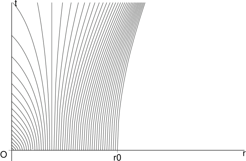
Figure 2: If $0<qE_{0}<q^{2}ar_{0}^{3}/30$, there is a radius value $r$ between 0 and $r_{0}$ for which $Q(r,t_{0})$ becomes zero. At this radius, the ball is stationary. The outer part expands because here the Coulomb repulsion of the dust particles is stronger than the Coulomb attraction of the point charge towards the origin; the inner part collapses because here it is vice versa. Again, any dust particle that reaches the origin arrives there at the speed of light, and the density $n(r,t)$ is singular at $r=0$ for all $t>t_{0}$.

 

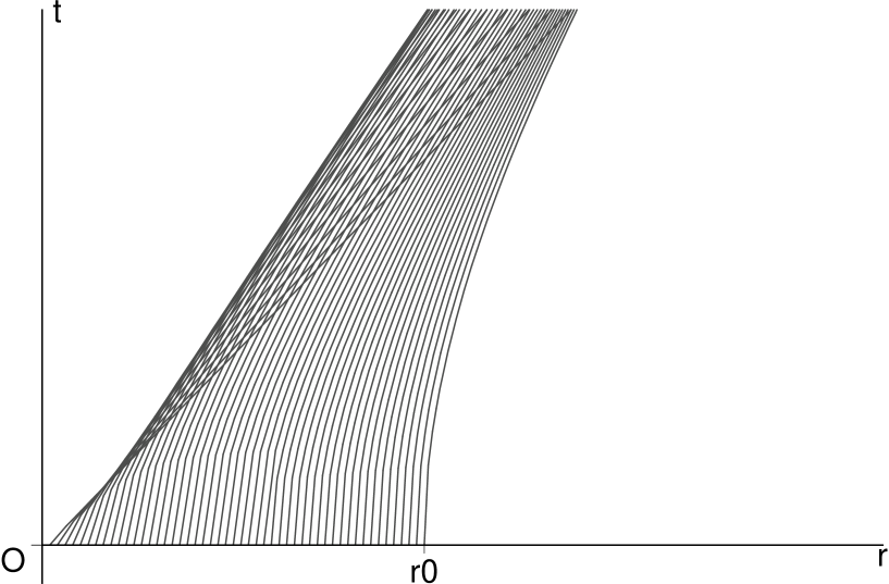
Figure 3: If $qE_{0}>q^{2}ar_{0}^{3}/30$, the point charge at the centre has the same sign as the charge of the dust, so it enhances the tendency of the dust to expand outwards. The inner parts of the ball move faster than the outer parts and overtake them, thereby forming a caustic. The solution to the Maxwell-Lorentz equations breaks down when flow lines cross over. As guaranteed by our general theorem, the solution is well-defined and unique on a neighborhood of the initial hypersurface. In this case, the latter is a snapshot of a punctured ball.

 

6 Conclusion

In this article we have demonstrated that the initial-value problem of the Maxwell-Lorentz equations is well-posed, and we have illustrated some qualitative features of these equations by studying spherically symmetric solutions on Minkowski spacetime. In view of applications, it is desirable to generalise our result in two directions. Firstly, one would like to include a pressure term into the equations, thereby allowing for situations where temperature and density are so high that the model of a “dust” (or “cold fluid”) is no longer applicable. Secondly, one would like to consider mixtures of two or more fluids which are dynamically coupled together. This would allow for considering two-fluid models of plasmas, treating both the electron component and the ion component as dynamical fields. In particular the first generalisation would require a considerable change in the mathematical techniques. Whereas for our treatment of a dust it was crucial that the density could be eliminated from the evolution equations, this would no longer be true for a fluid with pressure. One would have to use either the density or the pressure as an additional dynamical variable, and to eliminate the other one with the help of an equation of state. One would also expect that a pressure term would change the behaviour of a collapsing ball of charge. In particular, the somewhat pathological behaviour near the centre, as discussed in Chapter 5, is likely to be modified by a pressure term.

References

• [1] D. A. Burton, J. Gratus, and R. W. Tucker. Asymptotic analysis of ultra-relativistic charge. Ann. Phys. (NY), 322:599–630, 2007.
• [2] H. Spohn. Dynamics of charged particles and their radiation field. Cambridge University Press, Cambridge, 2004.
• [3] A. Komech and H. Spohn. Long-time asymptotics for the coupled Maxwell-Lorentz equations. Commun. Partial Diff. Equat., 25:559–584, 2000.
• [4] M. Kunze and H. Spohn. Adiabatic limit for the Maxwell-Lorentz equations. Ann. H. Poincaré, 1:625–654, 2000.
• [5] G. Bauer and D. Dürr. The Maxwell-Lorentz system of a rigid charge. Ann. H. Poincaré, 2:179–196, 2001.
• [6] S. Parrott. Relativistic electrodynamics and differential geometry. Springer, New York, 1987.
• [7] M. E. Taylor. Pseudodifferential operators and nonlinear PDE. Birkhäuser, Boston, 1991.
• [8] D. A. Burton, J. Gratus, and R. W. Tucker. Multiple currents in charged continua. J. Phys. A, 40:811–829, 2007.