Semi-classical signal analysis

Abstract:

This study introduces a new signal analysis method called SCSA, based on a semi-classical approach. The main idea in the SCSA is to interpret a pulse-shaped signal as a potential of a Schrödinger operator and then to use the discrete spectrum of this operator for the analysis of the signal. We present some numerical examples and the first results obtained with this method on the analysis of arterial blood pressure waveforms.

Keywords:

Signal analysis, Schrödinger operator, semi-classical, arterial blood pressure

AMS:

00A69, 94A12, 92C55

1 Introduction

This paper considers a new signal analysis method where the main idea is to interpret a signal $y$ as a multiplication operator, $\phi\rightarrow y.\phi$, on some function space. The spectrum of a (formally) regularized version of this operator, denoted $H_{h}(y)$ and defined by

$$H_{h}(y)\psi=-h^{2}\frac{d^{2}\psi}{dx^{2}}-y\psi,\quad\psi\in H^{2}(\mathbb{R}),\quad h>0,$$ (1)

for small $h$, is then used for the analysis instead of the Fourier transform of $y$. Here $H^{2}(\mathbb{R})$ denotes the Sobolev space of order 2. In this method, the signal is interpreted as a potential of a Schrödinger operator. This point of view seems useful when associated inverse spectral problem is well posed as it will be the case for some pulse shaped signals.

We define $H_{h}$ on a space $\mathcal{B}$ such that

$$\mathcal{B}=\{y\in L_{1}^{1}(\mathbb{R}),\quad y(x)\geq 0,\quad\forall x\in\mathbb{R},\quad\frac{\partial^{m}y}{\partial x^{m}}\in L^{1}(\mathbb{R}),\quad m=1,2\},$$ (2)

with, $\displaystyle{L_{1}^{1}(\mathbb{R})=\{V|\int_{-\infty}^{+\infty}{|V(x)|(1+|x|)dx}<\infty\}}$. $L_{1}^{1}(\mathbb{R})$ is known as the Faddeev class [9].

For $\lambda\leq 0$, we denote $N_{h}(\lambda;y)$ the number of eigenvalues of the operator $H_{h}(y)$ below $\lambda$. Under hypothesis (2), there is a non-zero finite number $N_{h}=N_{h}(0;y)$, as it is described in proposition 2.1. We denote $-\kappa_{nh}^{2}$ the negative eigenvalues of $H_{h}(y)$ with $\kappa_{nh}>0$ and $\kappa_{1h}>\kappa_{2h}>\cdots>\kappa_{nh}$, $n=1,\cdots,N_{h}$. Let $\psi_{nh}$, $n=1,\cdots,N_{h}$ be the associated $L^{2}$-normalized eigenfunctions.

In this study, we focus our interest in representing the signal $y$ with the discrete spectrum of $H_{h}(y)$ using the following formula (3)

$$y_{h}(x)=4h\sum_{n=1}^{N_{h}}{\kappa_{nh}\psi_{nh}^{2}(x)},\quad\quad x\in\mathbb{R}.$$ (3)

As we will see, the parameter $h$ plays an important role in our approach. Indeed, as $h$ decreases as the approximation of $y$ by $y_{h}$ improves. Our method is based on semi-classical concepts i.e $h\rightarrow 0$ and we will call it Semi-Classical Signal Analysis (SCSA).

In the next section, we will present some properties of the SCSA. In section 3, we will consider a particular case of an exact representation for a fixed $h$ and show its relation to a signal representation using the so called reflectionless potentials of the Schrödinger operator. Section 4 will deal with some numerical examples and section 5 will present some results obtained on the analysis of Arterial Blood Pressure (ABP) signals using the SCSA. A discussion will summarize the main results and compare the SCSA to related studies. In appendices A, B and C some known results on direct and inverse scattering transforms are presented.

2 SCSA properties

To begin, we focuss our attention on the behavior of the number $N_{h}$ of negative eigenvalues of $H_{h}(y)$ according to $h$ as described by the following proposition.

Proposition 2.1.

Let $y$ be a real valued function satisfying hypothesis (2). Then,

• The number $N_{h}$ of negative eigenvalues of $H_{h}(y)$ is a decreasing function of $h$.
  

• Moreover if $y\in L^{\frac{1}{2}}(\mathbb{R})$, then,

  $$\lim_{h\rightarrow 0}{hN_{h}}=\frac{1}{\pi}\int_{-\infty}^{+\infty}{\sqrt{y(x)}dx},$$ (4)

Proof.

• The proof of this item is based on the following lemma.

  Lemme 2.1.

  [2][28] For $\lambda\leq 0$, let $N_{1}(\lambda;V)$ be the number of negative eigenvalues of $H_{1}(V)$ less than $\lambda$. Let $V$ and $W$ be two potentials of the Schrödinger operator such that $W\leq V$, then

  $$N_{1}(\lambda;W)\leq N_{1}(\lambda;V),\quad\forall\lambda\leq 0.$$ (5)

  Let $y\in\mathcal{B}$. We put $\displaystyle{V=\frac{1}{h_{1}^{2}}y,\quad\quad W=\frac{1}{h_{2}^{2}}y,\quad\quad\mbox{with }\quad 0<h_{1}\leq h_{2}}$.

  For $\lambda=0$, we obtain $\displaystyle{N_{1}(0;\frac{1}{h_{2}^{2}}y)\leq N_{1}(0;\frac{1}{h_{1}^{2}}y),}$ and we have $N_{1}(0;\frac{1}{h_{j}^{2}}y)=N_{h_{j}}$, $j=1,2$, which proves the result.
  

• Let $y\in\mathcal{B}\cap L^{\frac{1}{2}}(\mathbb{R})$ and $\lambda\in]-y_{max},0]$. We denote

  $$S_{\gamma}(h,\lambda)=\sum_{\kappa_{nh}^{2}\leq\lambda}{\left(\lambda+\kappa_{nh}^{2}\right)^{\gamma}},\quad\quad\gamma\geq 0$$ (6)

  the Riesz means of the values $-\kappa_{nh}^{2}$ less than $\lambda$. Remark that $S_{0}(h,\lambda)=N_{h}(\lambda;y)$.

  Property ii) results from the following lemma 2.2

  Lemme 2.2.

  [23] For $y\in L^{\gamma+\frac{1}{2}}(\mathbb{R})$, $y(x)\geq 0$, $\forall x\in\mathbb{R}$ and $\gamma\geq 0$, we have

  $$\lim_{h\rightarrow 0}{hS_{\gamma}(h,0)}=L_{\gamma}^{cl}\int_{-\infty}^{+\infty}{y(x)^{\gamma+\frac{1}{2}}dx},$$ (7)

  where $L_{\gamma}^{cl}$ is the classical constant given by

  $$L_{\gamma}^{cl}=\frac{\Gamma(\gamma+1)}{2\sqrt{\pi}\Gamma(\gamma+\frac{3}{2})},$$ (8)

  for all $\gamma\geq 0$

  By taking $\gamma=0$ in (7) we get the result.

Let us now study some properties of the negative eigenvalues $-\kappa_{nh}^{2}$, $n=1,\cdots,N_{h}$ of $H_{h}(y)$.

Proposition 2.2.

Let $y\in C^{\infty}(\mathbb{R})$, with $y(x)>0$, $\forall x\in\mathbb{R}$ and such that $\exists\gamma_{0}\in\mathbb{R}$, $\min_{\mathbb{R}}{(-y+\gamma_{0})}>0$ and $\forall\alpha\in\mathbb{N}$, $\exists C_{\alpha}>0$ such that $|\frac{\partial^{\alpha}y}{\partial x^{\alpha}}|\leq C_{\alpha}(-y+\gamma_{0})$, then every regular value of $y$ is an accumulation point of the set ($\kappa_{nh}^{2}$, $n=1,\cdots,N_{h}$) ($v$ is a regular value if $0<v<y_{max}$ and if $y(x)=v$ then $|\frac{dy(x)}{dx}|>0$).

Proof.

We want to show that every regular value of $y$ is an accumulation point for the set ($\kappa_{nh}^{2}$, $n=1,\cdots,N_{h}$). For this purpose, we use the following result shown by B. Helffer and D. Robert [14].

Theorem 2.1.

[14] Let $y\in C^{\infty}(\mathbb{R})$, with $y(x)>0$, $\forall x\in\mathbb{R}$ such that for $\gamma_{0}\in\mathbb{R}$, $\min_{\mathbb{R}}{(-y+\gamma_{0})}>0$ and for all $\alpha\in\mathbb{N}$, there is a constant $C_{\alpha}>0$ such that $|\frac{\partial^{\alpha}y}{\partial x^{\alpha}}|\leq C_{\alpha}(-y+\gamma_{0})$. Let $\lambda<\lim\inf_{|x|\rightarrow\infty}({-y(x)})$, then for $0\leq\gamma\leq 1$ the Riesz means (6) are given by

$$S_{\gamma}(h,\lambda)=\frac{1}{h}\left(L_{\gamma}^{cl}\int_{-\infty}^{+\infty}{\left|\lambda+y(x)\right|_{+}^{\gamma+\frac{1}{2}}dx}+O(h^{1+\gamma})\right),$$ (9)

where $|V|_{+}$ is the positive part of $V$ and $L_{\gamma}^{cl}$, known as the classical constant, is given by (8).

We put $\gamma=0$ in (6). We notice that $S_{0}(h,\lambda)=N_{h}(\lambda,y)$. Substituting $\gamma$ by $0$ in (9), we get

$$S_{0}(h,\lambda)=\frac{1}{h}L_{0}^{cl}\int_{-\infty}^{+\infty}{\sqrt{\left|\lambda+y(x)\right|_{+}}dx}+O(1).$$ (10)

We suppose that there is a regular value $y_{0}$ of $y$ that is not an accumulation point of the set ($\kappa_{nh}^{2}$, $n=1,\cdots,N_{h}$). So there is a neighborhood $V(y_{0})$ of $y_{0}$ and a value $h_{0}$, small enough such that $\forall h<h_{0}$, $V(y_{0})$ does not contain any element element $\kappa_{nh}^{2}$.

Moreover, we can choose $V(y_{0})$ small enough such that

$$\inf\{|\frac{dy(x)}{dx}|,\quad\mbox{for}\quad x\quad\mbox{such that}\quad y(x)\in V(y_{0})\}=c>0.$$ (11)

Then, we can take $V(y_{0})=[y_{1},y_{2}[$, with $y_{1}$ and $y_{2}$ some regular values of $y$ and $0<y_{1}<y_{2}$.

For all $h<h_{0}$, the difference $S_{0}(h,-y_{1})-S_{0}(h,-y_{2})$ represents the number of elements of ($-\kappa_{nh}^{2}$, $n=1,\cdots,N_{h}$) in the interval $]-y_{2},-y_{1}]$. However this set is empty because there is no element in the neighborhood of $y_{0}$.

Denoting $X(\lambda)=\{x|y(x)+\lambda\geq 0\}$, we have from (10)

$$\!\!\!S_{0}(h,-y_{1})\!-\!S_{0}(h,-y_{2}) = \frac{1}{h}L_{0}^{cl}\!\left(\int_{X(-y_{1})}{\!\!\!\!\!\!\!\!\sqrt{y(x)-y_{1}}dx}\!-\!\int_{X(-y_{2})}{\!\!\!\!\!\!\!\!\sqrt{y(x)-y_{2}}dx}\right)\!\!$$ (12)

$$+ \!\!O(1),\!$$

so, as the left quantity is null, we obtain

$$\int_{X(-y_{1})}{\sqrt{y(x)-y_{1}}dx}=\int_{X(-y_{2})}{\sqrt{y(x)-y_{2}}dx},$$ (13)

and we have $X(-y_{1})=X(-y_{2})\cup y^{-1}([y_{1},y_{2}[)$, so

$$\int_{X(-y_{2})}{\!\!\!\!\!\!\!\!\!\sqrt{y(x)-y_{1}}dx}+\int_{y^{-1}([y_{1},y_{2}[)}{\!\!\!\!\!\!\!\!\!\sqrt{y(x)-y_{1}}dx}=\int_{X(-y_{2})}{\!\!\!\!\!\!\!\!\!\sqrt{y(x)-y_{2}}dx},$$ (14)

$$\int_{X(-y_{2})}{(\sqrt{y(x)-y_{1}}-\sqrt{y(x)-y_{2}})dx}+\int_{y^{-1}([y_{1},y_{2}[)}{\sqrt{y(x)-y_{1}}dx}=0.$$ (15)

Hence as these two integrals are positives, we get

$$\int_{y^{-1}([y_{1},y_{2}[)}{\sqrt{y(x)-y_{1}}dx}=0,$$ (16)

therefore $|y(x)-y_{1}|=0$ almost everywhere in $y^{-1}([y_{1},y_{2}[)$, then $y_{1}=y_{2}$, which is a contradiction.

Now, proposition 2.2 introduces an interesting property of the SCSA. Indeed, remembering that

$$-h^{2}\frac{d^{2}\psi_{nh}(x)}{dx^{2}}-y(x)\psi_{nh}(x)=-\kappa_{nh}^{2}\psi_{nh}(x).$$ (17)

and by multiplying the previous equation by $\psi_{nh}(x)$ and integrating it by part we get

$$\kappa_{nh}^{2}=\int_{-\infty}^{+\infty}{y\psi_{nh}^{2}(x)dx}-h^{2}\int_{-\infty}^{+\infty}{\left(\frac{d\psi_{nh}(x)}{dx}\right)^{2}dx}.$$ (18)

Then, we notice that $-y_{max}\leq-\kappa_{nh}^{2}<0$ as it is illustrated in figure 1. Hence, for a fixed value of $h$, $\kappa_{nh}^{2}$ can be interpreted as particular values of $y$ which define a new quantization approach that can be interpreted by semi-classical concepts. The SCSA appears then as a new way to quantify a signal.

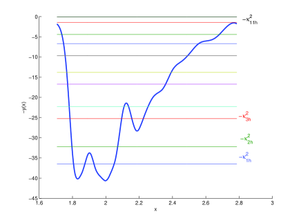
Figure 1: The negative spectrum of the Schrödinger operator $-h^{2}\dfrac{d^{2}}{dx^{2}}-y(x)$ provides a quantization of the signal $y$

To finish this section, we examine the convergence of the first two momentums of $\kappa_{nh}$ when $h\rightarrow 0$ through proposition 2.3. These quantities could be very interesting in signal analysis as it is mentioned in section 5 and also in a recent study [20].

Proposition 2.3.

Under hypothesis (2), we have

$$\lim_{h\rightarrow 0}{h\sum_{n=1}^{N_{h}}{\kappa_{nh}}}=\frac{1}{4}\int_{-\infty}^{+\infty}{y(x)dx},$$ (19)

and remembering that

$$y_{h}(x)=4h\sum_{n=1}^{N_{h}}{\kappa_{nh}\psi_{nh}^{2}(x)},\quad\quad x\in\mathbb{R},$$ (20)

we have

$$\lim_{h\rightarrow 0}\int_{-\infty}^{+\infty}{y_{h}(x)dx}=\int_{-\infty}^{+\infty}{y(x)dx}.$$ (21)

Moreover if $y\in L^{2}(\mathbb{R})$, then,

$$\lim_{h\rightarrow 0}{h\sum_{n=1}^{N_{h}}{\kappa_{nh}^{3}}}=\frac{3}{16}\int_{-\infty}^{+\infty}{y^{2}(x)dx}.$$ (22)

Proof. The limits (19) and (22) are deduced from lemma 2.2 for $\gamma=\dfrac{1}{2}$ and $\gamma=\dfrac{3}{2}$ respectively,

$$\lim_{h\rightarrow 0}{h\sum_{n=1}^{N_{h}}{\kappa_{nh}}}=\frac{1}{4}\int_{-\infty}^{+\infty}{y(x)dx},$$ (23)

$$\lim_{h\rightarrow 0}{h\sum_{n=1}^{N_{h}}{\kappa_{nh}^{3}}}=\frac{3}{16}\int_{-\infty}^{+\infty}{y^{2}(x)dx}.$$ (24)

By integrating (3) we have

$$\int_{-\infty}^{+\infty}{y_{h}(x)dx}=4h\sum_{n=1}^{N_{h}}{\kappa_{nh}}.$$ (25)

Then, combining (25) and (19), we get (21).

3 Exact representation and reflectionless potentials

In this section, we are interested in an exact representation of a signal for a fixed $h$ and its relation to reflectionless potentials (reflectionless potentials are defined in the appendix B) of the Schrödinger operator as it is described in the following proposition:

Proposition 3.1.

The following properties are equivalent,

• Equality in (19) holds for a finite $h$ ;

• $\exists h$ such that $y_{h}=y$ ;

• $\exists h$ such that $\dfrac{y}{h^{2}}$ is a reflectionless potential of $H_{1}(V)$.

Proof

The following proof uses some concepts and results from scattering transform theory that are recalled in the appendix. First, we suppose that i) is fulfilled then

$$\exists h,\quad\int_{-\infty}^{+\infty}{y(x)dx}=4h\sum_{n=1}^{N_{h}}{\kappa_{nh}}.$$ (26)

Writing the first invariant 60 (see the appendix C) for the potential $-\dfrac{y}{h^{2}}$ we have

$$\int_{-\infty}^{+\infty}{y(x)dx}=4h\sum_{n=1}^{N_{h}}{\kappa_{nh}}+\frac{h^{2}}{\pi}\int_{-\infty}^{+\infty}{\ln{(1-|R_{r(l)h}(k)|^{2})}dk},$$ (27)

where $R_{r(l)h}(k)$ is the reflection coefficient (see the appendix A).

Using (25), we get

$$\int_{-\infty}^{+\infty}{y(x)dx}=\int_{-\infty}^{+\infty}{y_{h}(x)dx}+\frac{h^{2}}{\pi}\int_{-\infty}^{+\infty}{\ln{(1-|R_{r(l)h}(k)|^{2})}dk}.$$ (28)

Then, from (30) and (28) we obtain

$$\int_{-\infty}^{+\infty}{\ln{(1-|R_{r(l)h}(k)|^{2})}dk}=0.$$ (29)

The reflection coefficient of a Schrödinger operator satisfies $|R_{r(l)h}(k)|\leq 1$, $\forall k\in\mathbb{R}$ (see for exemple [6]). Then, we get $\ln{(1-|R_{r(l)h}(k)|^{2})}\leq 0$. Equality (29) is then fulfilled if and only if $\ln{(1-|R_{r(l)h}(k)|^{2})}=0$, $k\in\mathbb{R}\>\>a.e$; which is true only if $|R_{r(l)h}(k)|=0$, $k\in\mathbb{R}\>\>a.e$. This property defines a reflectionless potential. So, $i)\Rightarrow iii)$.

Now, using the Deift-Trubowitz formula (56) (see appendix B) that we rewrite for the potential $-\dfrac{y}{h^{2}}$ and taking $R_{r(l)h}(k)=0$, we can deduce that statement (iii) implies statement (ii).

Then, if we suppose that $y_{h}=y$ for a given value of $h$ we have

$$\int_{-\infty}^{+\infty}{y_{h}(x)dx}=\int_{-\infty}^{+\infty}{y(x)dx},$$ (30)

hence $ii)\Rightarrow i)$

4 Numerical results

In this section, we are interested in the validation of the SCSA through some numerical examples. For this purpose, it will be more convenient to consider the problem associated to $H_{1}(\dfrac{y}{h^{2}})$. Therefore, in order to simplify the notations, we put $\dfrac{1}{h^{2}}=\chi$, $N_{h}=N_{\chi}$ and $\dfrac{\kappa_{nh}^{2}}{h^{2}}=\kappa_{n\chi}^{2}$, $n=1,\cdots,N_{\chi}$. We denote the $L^{2}$-normalized eigenfunctions $\psi_{n\chi}$, $n=1,\cdots,N_{\chi}$. Formula (3) is then rewritten

$$y_{\chi}(x)=\frac{4}{\chi}\sum_{n=1}^{N_{\chi}}{\kappa_{n\chi}\psi_{n\chi}^{2}(x)},\quad\quad x\in\mathbb{R},$$ (31)

We start by giving the numerical scheme used to estimate a signal with the SCSA. Then, the sech-squared function will be considered. This example illustrates the influence of the parameter $\chi$ on the approximation. Gaussian, sinusoidal and chirp signals will be also considered.

4.1 The numerical scheme

The first step in the SCSA is to solve the spectral problem of a one dimensional Schrödinger operator. Its discretization leads to an eigenvalue problem of a matrix. In this work, we propose to use a Fourier pseudo-spectral method [15], [30]. The latter is well-adapted for periodic problems but in practice it gives good results for some non-periodic problems for instance, rapid decreasing signals.

We consider a grid of $M$ equidistant points $x_{j}$, $j=1,\cdots,M$ such that

$$a=x_{1}<x_{2}<\cdots<x_{M-1}<x_{M}=b.$$ (32)

Let $\Delta x=\dfrac{b-a}{M-1}$ be the distance between two consecutive points. We denote $y_{j}$ and $\psi_{j}$ the values of $y$ and $\psi$ at the grid points $x_{j}$, $j=1,\cdots,M$

$$y_{j}=y(x_{j}),\quad\psi_{j}=\psi(x_{j}),\quad j=1,\cdots,M.$$ (33)

Therefore, the discretization of the Schrödinger eigenvalue problem leads to the following eigenvalue matrix problem

$$\left(-D_{2}-\chi\operatorname{diag}\left(Y\right)\right)\underline{\psi}=\-\lambda\underline{\psi},$$ (34)

where $\operatorname{diag}(Y)$ is a diagonal matrix whose elements are $y_{j}$, $j=1,\cdots,M$ and $\underline{\psi}=\left[\psi_{1}\>\>\psi_{2},\>\>\cdots\>\>\psi_{M-1}\>\>\psi_{M}\right]^{T}$. $D_{2}$ is the second order differentiation matrix given by [30],

• If $M$ is even

  $$D_{2}(k,j)=\frac{\Delta^{2}}{(\Delta x)^{2}}\left\{\begin{array}[]{ll}\dfrac{-\pi^{2}}{3\Delta^{2}}-\dfrac{1}{6}&\quad\mbox{for}\>\>k=j,\\ -\left(-1\right)^{k-j}\dfrac{1}{2}\dfrac{1}{\sin^{2}{\left(\frac{\left(k-j\right)\Delta}{2}\right)}}&\quad\mbox{for}\>\>k\neq j.\\ \end{array}\right.$$ (35)

• If $M$ is odd

  $$D_{2}(k,j)=\frac{\Delta^{2}}{(\Delta x)^{2}}\left\{\begin{array}[]{ll}\dfrac{-\pi^{2}}{3\Delta^{2}}-\dfrac{1}{12}&\quad\mbox{pour}\>\>k=j,\\ -\left(-1\right)^{k-j}\dfrac{1}{2}\dfrac{1}{\sin{\left(\frac{\left(k-j\right)\Delta}{2}\right)}}\cot{\left(\frac{\left(k-j\right)\Delta}{2}\right)}&\quad\mbox{pour}\>\>k\neq j,\\ \end{array}\right.$$ (36)

with $\Delta=\dfrac{2\pi}{M}$. the matrix $D_{2}$ is symmetric and definite negative. To solve the eigenvalue problem of the matrix $(-D_{2}-\chi\operatorname{diag}(Y))$ we use the Matlab routine eig.

The final step in the SCSA algorithm is to find an optimal value of the parameter $\chi$. So we look for a value $\hat{\chi}$ that gives a good approximation of $y$ with a small number of negative eigenvalues. From the numerical tests, we noticed that the number $N_{\chi}$ is in general a step by step function of $\chi$. So, we optimize the following criteria in each interval $\left[\chi_{1},\chi_{2}\right]$ where $N_{\chi}$ is constant,

$$J(\chi)=\frac{1}{M}\sum_{i=1}^{M}{\left(y_{i}-y_{\chi i}\right)^{2}},\quad y_{\chi i}=\frac{4}{\chi}\sum_{n=1}^{N_{\chi}}{\kappa_{n\chi}\psi_{ni\chi}^{2}},\quad i=1,\cdots,M.$$ (37)

For $\chi$ large enough (equivalently $h$ small enough), we know an approximate relation between the number of negative eigenvalues and $\chi$ thanks to proposition 2.1. Then, we can deduce approximate values of $\chi_{1}$ and $\chi_{2}$ according to a given number of negative eigenvalues. Fig. 2 summarizes the SCSA algorithm.

Figure 2: The SCSA algorithm

Remark: In practice, we often omit the optimization step and just fix $N_{\chi}$ to a large enough value.

4.2 The sech-squared function

In order to illustrate the influence of the parameter $\chi$ on the SCSA, we first study a sech-squared function given by

$$y(x)=\operatorname{sech}^{2}(x-x_{0}),\quad x\in\mathbb{R}.$$ (38)

The potential of the Schrödinger operator $H_{1}(\chi y)$ is given in this case by: $-\chi\operatorname{sech}^{2}(x-x_{0})$. This potential is called in quantum physics Pöschl-Teller potential.

It is well-known that the Pöschl-Teller potential belongs to the class of reflectionless potentials if,

$$\chi=\chi_{p}=N(N+1),\quad\quad N=1,2,3,\cdots,$$ (39)

$N$ being the number of negative eigenvalues of $H_{1}(\chi y)$ [22].

So, for example, if $\chi=2$, the Schrödinger operator spectrum is negative and consists of a single negative eigenvalue given by $\lambda=-1$. If $\chi=6$, there are two negative eigenvalues: $\lambda_{1}=-4$, $\lambda_{2}=-1$ and so on.

Let us now apply the SCSA to reconstruct $y$. For this purpose, we must truncate the signal and consider it on a finite interval so that the numerical computations could be possible.

Figure 3.a illustrates the variation of the mean square error and $N_{\chi}$ according to $\chi$. We notice that,

• $N_{\chi}$ is an increasing function of $\chi$ as described in proposition (2.1). Moreover, $N_{\chi}$ is a step by step function.
  

• There are some particular values of $\chi$ for which the error is minimal. These values are in fact the particular values $\chi_{p}=N_{\chi}(N_{\chi}+1)$, $N_{\chi}=1,2,\cdots$ for which $-\chi y$ is a reflectionless potential.
  

• For all $\epsilon>0$, there is a value $\chi=\chi_{\epsilon}$ such that $\forall\chi>\chi_{\epsilon},\quad J(\chi)<\epsilon$.
  

Figure 3.b illustrates the variation of the first four eigenvalues of the matrix $-D_{2}-\chi\operatorname{diag}(Y)$, settled in an increasing way, according to $\chi$. We notice that these eigenvalues, initially positive, are decreasing functions of $\chi$ and at every passage from $N_{\chi}$ to $N_{\chi}+1$, a positive eigenvalue becomes negative.

Otherwise, in figure 4, the first four squared eigenfunctions $\psi_{n\chi}^{2}$, $n=1,\cdots,4$ are represented for $\chi=20$. Each $\psi_{n\chi}^{2}$ has $n-1$ zeros.

Figure 5 shows a satisfactory reconstruction of $y$ for $N_{\chi}=1,2,3$ and $4$.

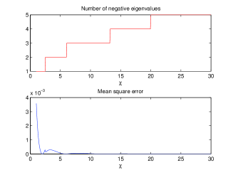
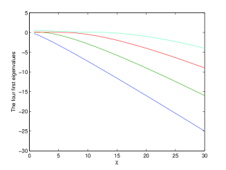
(a)                                             (b)

Figure 3: (a) Mean square error and number of negative eigenvalues according to $\chi$ for $y(x)=\operatorname{sech}^{2}(x-6)$ in $\left[0,15\right]$. (b) Four first eigenvalues according to $\chi$ for $y(x)=\operatorname{sech}^{2}(x-6)$ in $\left[0,15\right]$

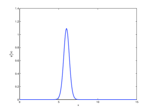
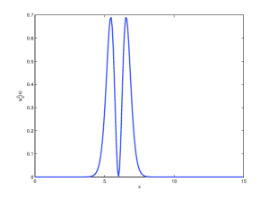
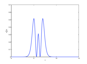
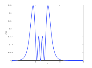
Figure 4: Four first eigenfunctions $\psi_{n\chi}^{2}$ for $\chi=20$ for $y(x)=\operatorname{sech}^{2}(x-6)$ in $\left[0,15\right]$

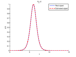
Figure 5: Estimation of $y(x)=\operatorname{sech}^{2}(x-6)$ in $\left[0,15\right]$, from the left to the right: $N_{\chi}=1$, $N_{\chi}=2$ (top). $N_{\chi}=3$, $N_{\chi}=4$ (bottom)

4.3 Estimation of some signals

In this section, we are interested in the estimation of some signals with the SCSA. In each case, we represent the estimation error, the number of negative eigenvalues according to $\chi$ and the real and estimated signals for different values of $\chi$.

We start with a gaussian signal given by:

$$y(x)=\frac{1}{\sigma\sqrt{2\pi}}e^{-\frac{(x-\mu)^{2}}{2\sigma^{2}}}.$$ (40)

For the numerical tests we take $\sigma=0.1$ and $\mu=0.75$.

Figures 6 and 7 illustrate the results. We notice that with $N_{\chi}=2$, the estimation is satisfactory and as $N_{\chi}$ increases better is the approximation.

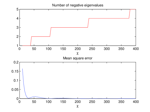
Figure 6: Mean square error and number of negative eigenvalues according to $\chi$ for a gaussian signal

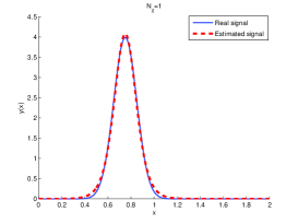
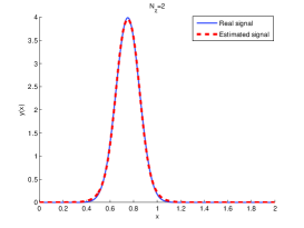
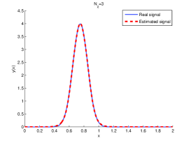
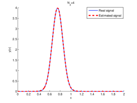
Figure 7: Estimation of a gaussian signal, from the left to the right: $N_{\chi}=1$, $N_{\chi}=2$ (top). $N_{\chi}=3$, $N_{\chi}=4$ (bottom)

Now we are interested in a sinusoidal signal defined in a finite interval $I$,

$$y(x)=\left\{\begin{array}[]{cc}A\sin(\omega x+\phi)&x\in I\\ 0&\mbox{otherwise}\\ \end{array}\right.$$ (41)

This signal has negative values, so to apply the SCSA, we must translate the signal by $y_{min}=-A$ such that $y-y_{min}>0$. The Schrödinger operator potential to be considered is then given by $-\chi(y-y_{min})$. For the numerical tests, we took $A=2$, $\omega=\pi$ and $\phi=-0.5$.

The results are represented in figures 8, 9 and 10. In 9, a single period of the signal is considered while in 10, four periods are represented. In the last case we noticed that the negative eigenvalues are of multiplicity 4, they are repeated in each period.

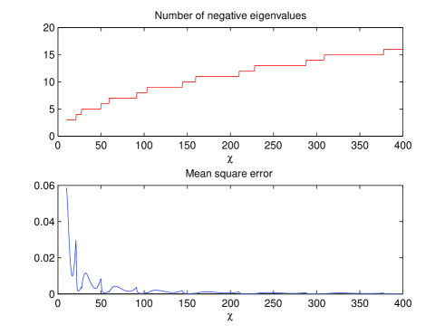
Figure 8: Mean square error and number of negative eigenvalues according to $\chi$ for a sinusoidal signal

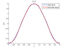
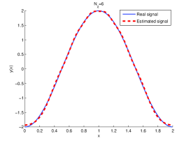
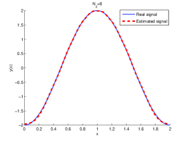
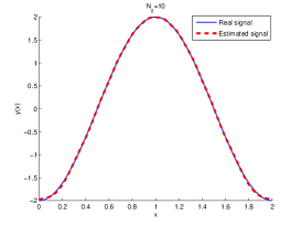
Figure 9: Estimation of a sinusoidal signal, from the left to the right: $N_{\chi}=4$, $N_{\chi}=6$ (top). $N_{\chi}=8$, $N_{\chi}=10$ (bottom)

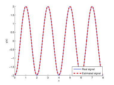
Figure 10: Estimation of 4 sinusoidal signal periods with $N_{\chi}=10$

Finally, figures 11 and 12 illustrate the results obtained in the case of a chirp signal. We recall that a chirp signal is usually defined by a time varying frequency sinusoid. In our tests, we considered a linear variation of the frequency.

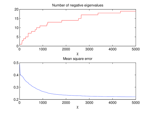
Figure 11: Mean square error and number of negative eigenvalues according to $\chi$ for a chirp signal

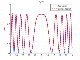
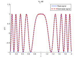
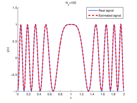
Figure 12: Estimation of a chirp signal, from the left to the right: $N_{\chi}=30$, $N_{\chi}=50$ (top). $N_{\chi}=80$, $N_{\chi}=100$ (bottom)

5 Arterial blood pressure analysis with the SCSA

ABP plays an important role in the cardiovascular system. So many studies were done aiming at proposing mathematical models in order to understand the cardiovascular system both in healthy and pathological cases. Despite the large number of ABP models, the interpretation of ABP in clinical practice is often restricted to the interpretation of the maximal and the minimal values called respectively the systolic pressure and the diastolic pressure. None information on the instantaneous variability of the pressure is given in this case. However, pertinent information can be extracted from ABP waveform. The SCSA seems to provide a new tool for the analysis of ABP waveform. This section presents some obtained results.

We denote the ABP signal $P$ and $\hat{P}$ its estimation using the SCSA such that

$$\hat{P}(t)=\frac{4}{\chi}\sum_{n=1}^{N_{\chi}}{\kappa_{n\chi}\psi_{n\chi}^{2}(t)},$$ (42)

where $-\kappa_{n\chi}^{2}$, $n=1,\cdots,N_{\chi}$ are the $N_{\chi}$ negative eigenvalues of $H_{1}(\chi P)$ and $\psi_{n\chi}$ the associated $L^{2}-$normalized eigenfunctions. As ABP signal is a function of time, we use the time variable $t$ in the Schrödinger equation instead of the space variable $x$.

The ABP signal was estimated for several values of the parameter $\chi$ and hence $N_{\chi}$. Figure 13 illustrates the measured and estimated pressures for one beat of ABP and the estimated error with $N_{\chi}=9$. Signals measured at the aorta level and the finger respectively were considered. We point out that $5$ to $9$ negative eigenvalues are sufficient for a good estimation of ABP signals [17], [19].

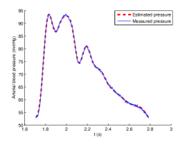
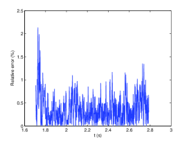
(a) Aorta

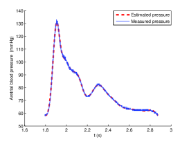
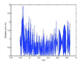
(b) Finger

Figure 13: Reconstruction of the pressure at the aorta and the finger level with the SCSA and $N_{\chi}=9$. On the left the estimated and measured pressures, On the right the relative error

A first interest in using the SCSA for ABP analysis is to decompose the signal into its systolic and diastolic parts respectively. This application was inspired from a reduced model of ABP based on solitons introduced in [4], [18]. Solitons are in fact solutions of some nonlinear partial derivative equations for instance the Korteweg-de Vries (KdV) equation which was considered in this reduced model [4]. This model proposes to write the ABP as the sum of two terms: and N-soliton, solution of the KdV equation describing fast phenomena that predominate during the systolic phase and a two-elements windkessel model that describes slow phenomena during the diastolic phase. Moreover the KdV equation can be solved with the Inverse Scattering Transform (IST) whose definition is recalled in appendix A. In this approach, the KdV equation is associated to a one dimensional Schrödinger potential parameterized by time where the potential is given by the solution of the KdV equation at a given time. Therefore a relation between the Schrödinger operator and solitons was found [10]: solitons are reflectionless potentials. Then according to proposition 3.1, the SCSA coincides with a soliton representation of a signal for a finite $\chi$ when $-\chi y$ is an $N_{\chi}$-soliton, where $N_{\chi}$ denotes the number of negative eigenvalues of $H_{1}(\chi y)$. So each spectral component represents a single soliton. We know that solitons are characterized by their velocity which is determined by the negative eigenvalues $-\kappa_{n\chi}^{2}$, $n=1,\cdots,N_{\chi}$ of the Schrödinger operator. The largest values $\kappa_{n\chi}$ characterize fast components and the small values of $\kappa_{n\chi}$ characterize slow components. From these remarks, we propose to decompose equation (31) into two partial sums: the first one, composed of the $N_{s}$ ($N_{s}=1,2,3$ in general) largest $\kappa_{n\chi}$ and the second partial sum composed of the remaining components. The first partial sum describes the systolic phase and the second one describes the diastolic phase. We denote $\hat{P}_{s}$ and $\hat{P}_{d}$ the systolic pressure and the diastolic pressure respectively estimated with the SCSA. Then we have

$$\hat{P}_{s}(t)=\frac{4}{\chi}\sum_{n=1}^{N_{s}}{\kappa_{n\chi}\psi_{n\chi}^{2}(t)},\quad\quad\quad\hat{P}_{d}(t)=\frac{4}{\chi}\sum_{n=N_{s}+1}^{N_{\chi}}{\kappa_{n\chi}\psi_{n\chi}^{2}(t)}.$$ (43)

Figure 14 represents the measured pressure and the estimated systolic and diastolic pressures respectively. We notice that $\hat{P}_{s}$ and $\hat{P}_{d}$ are respectively localized during the systole and the diastole.

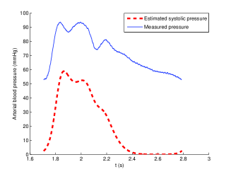
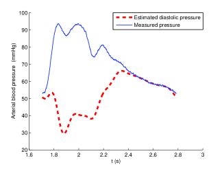
Figure 14: On the left the estimated systolic pressure. On the right estimated diastolic pressure

6 Discussion

The spectral analysis of the Schrödinger operator introduces two inverse problems: an inverse spectral problem and an inverse scattering problem.

On the one hand, the inverse spectral problem aims at reconstructing the potential of a Schrödinger operator with its spectrum (spectral function). It has been extensively studied for instance by Borg, Gel’Fand, Levitan and Marchenko [11] or more recently by Ramm [27]. They considered the half-line case and used two spectra of the Schrödinger operator with two different boundary conditions in order to reconstruct the potential. The inverse spectral problem for a semi-classical Schrödinger operator $H_{h}(y)$ have been recently considered for example by Colin de Verdiére [5] who proposed to reconstruct the potential locally with a single spectrum or Guillemin and Uribe [13] who showed that under some assumptions, the low-lying eigenvalues of the operator determine the Taylor series of the potential at the minimum.

In this work we have studied an inverse spectral approach that is different from classical inverse spectral problems. Indeed, we used more information to reconstruct the potential by including the eigenfunctions as illustrated by equation (3).

On the other hand, the inverse scattering problem aims at recovering the potential from the scattering data (see appendix A). Many studies considered this question for instance those of Marchenko [25] who proved that under some conditions on the scattering data, a potential in $L_{1}^{1}(\mathbb{R})$ can be reconstructed from these scattering data and gave an algorithm for recovering the potential. We can also quote works of Faddeev [9], Deift and Trubowitz [6] considering potentials in $L_{1}^{1}(\mathbb{R})$, Dubrovin, Matveev and Novikov [7] for periodic potentials.

The convergence of the SCSA when $h\rightarrow 0$ is not easy to study. Using the Deift-Trubowitz formula (56) we have tried to consider this problem. However, despite interesting results obtained regarding the convergence of some quantities depending only on the continuous spectrum of the Schrödinger operator to zero, we did not succeed in finding a result of convergence for $y_{h}$. A study supported by semi-classical concepts is now under consideration. The latter is based on the generalization of the results of G. Karadzhov [16].

The SCSA method has given promising results in the analysis of arterial blood pressure waveforms. More than a good reconstruction of these signals, the SCSA introduces interesting parameters that give relevant physiological information. These parameters are the negative eigenvalues and the invariants which are given by the momentums of $\kappa_{n\chi}$, $n=1,\cdots,N_{\chi}$ introduced in proposition 2.3. For example, these new cardiovascular indices allow the discrimination between healthy patients and heart failure subjects [21]. A recent study [20] shows that the first systolic momentum (associated to the systolic phase) gives information on stroke volume variation, a physiological parameter of great interest.

We have seen in proposition 3.1 that for a fixed value of $h$ the SCSA coincides with a reflectionless potentials approximation. This point seems to be an interesting avenue of research. Indeed, thanks to the relation between reflectionless potentials and solitons, the approximation by reflectionless potentials could have interesting applications in signal analysis and in particular in data compression. As we said in the previous section, solitons are reflectionless potentials of the Schrödinger operator. Gardner et al [10] showed that an $N$-soliton is completely determined by the discrete scattering data and in particular by $2N$ parameters which are the negative eigenvalues and the normalizing constants. Hence, if $-\chi y$ is an $N_{\chi}$-soliton, it is given by the following formula:

$$y(x)=\frac{2}{\chi}\frac{\partial^{2}}{\partial x^{2}}\ln{(\det{(I+A_{\chi})}})(x),\quad x\in\mathbb{R},$$ (44)

$A_{\chi}(x)$ is an $N_{\chi}\!\times\!N_{\chi}$ matrix of coefficients

$$A_{\chi}(x)=\left[\frac{c_{m\chi}c_{n\chi}}{\kappa_{m\chi}\!+\!\kappa_{n\chi}}e^{-(\kappa_{m\chi}\!+\!\kappa_{n\chi})x}\right]_{n,m},\quad n,m=1,\cdots,N_{\chi},$$ (45)

where $-\kappa_{n\chi}^{2}$ and $c_{n\chi}$, $n=1,\cdots,N_{\chi}$ are the negative eigenvalues and the normalizing constants of $H_{1}(\chi y)$. Hence, this formula provides a parsimonious representation of a signal.

The convergence of the approximation by solitons (or reflectionless potentials) when $\chi\rightarrow+\infty$ (equivalently $h\rightarrow 0$) was studied by Lax and Levermore [24] in a different context. Indeed they studied the small dispersion limit of the KdV equation and approached the initial condition of the KdV equation by an $N$-soliton that depends on the small dispersion parameter which is in our case $h$. They showed the results in the mono-well potential case and affirmed without prove that the result remain still true for multi-well potentials. However the main limitation of this approach is the difficulty to compute the normalizing constants. This difficulty can be explained by the fact that these constants are defined at infinity which can not be handled in the numerical implementation. At the best of our knowledge there is no study enabling the computation of these parameters apart a recent attempt by Sorine et al [29].

7 Conclusion

A new method for signal analysis based on a semi-classical approach has been proposed in this study: the signal is considered as a potential of a Schrödinger operator and then represented using the discrete spectrum of this operator. Some spectral parameters are then computed leading to a new approach for signal analysis. This study is a first step in the validation of the SCSA. Indeed, we have assessed here the ability of the SCSA to reconstruct some signals. We have studied particularly a challenging application which is the analysis of the arterial blood pressure waveforms. The SCSA introduces a novel approach for arterial blood pressure waveform analysis and enables the estimation of relevant physiological parameters. A theoretical study is now under consideration regarding the convergence of the SCSA for $h\rightarrow 0$. The work must be orientated at a second step to the comparison between the performance of the SCSA and other signal analysis methods like Fourier transform or the wavelets and also to the generalization of the SCSA to other fields.

Appendix A Direct and inverse scattering transforms

These appendices recall some known concepts on direct and inverse scattering transforms of a one-dimensional Schrödinger operator. For more details, the reader can refer to the large number of references on this subject for instance [1], [3], [6], [8], [9].

We consider here the spectral problem of a Schrödinger operator $H_{1}(-V)$, given by

$$-\frac{d^{2}\psi}{dx^{2}}+V(x,t)\psi=k^{2}\psi,\quad k\in\overline{\mathbb{C}}^{+},\quad x\in\mathbb{R},$$ (46)

where the potential $V$ such that $V\in\mathcal{B}$. For simplicity, we will omit the indice $1$ of the spectral parameters in the following.

For $k^{2}>0$, we introduce the solutions $\psi_{\pm}$ of equation (46) such that

$$\psi_{-}(k,x) = \left\{\begin{array}[]{lc}T(k)e^{-ikx}&\hskip 14.22636ptx\rightarrow-\infty,\\ e^{-ikx}+R_{r}(k)e^{+ikx}&\hskip 14.22636ptx\rightarrow+\infty,\\ \end{array}\right.$$ (49)

$$\psi_{+}(k,x) = \left\{\begin{array}[]{lc}T(k)e^{+ikx}&\hskip 14.22636ptx\rightarrow+\infty,\\ e^{+ikx}+R_{l}(k)e^{-ikx}&\hskip 14.22636ptx\rightarrow-\infty,\\ \end{array}\right.$$ (52)

where $T(k)$ is called the transmission coefficient and $R_{l(r)}(k)$ are the reflection coefficients from the left and the right respectively. The solution $\psi_{-}$ for example describes the scattering phenomenon for a wave $e^{-ikx}$ of amplitude $1$, sent from $+\infty$. This wave hit an obstacle which is the potential so that a part of the wave is transmitted $T(k)e^{-ikx}$ and the other part is reflected $R_{r}(k)e^{+ikx}$. $\psi_{+}$ describes the scattering phenomenon for a wave $e^{+ikx}$ sent from $-\infty$.

For $k^{2}<0$, the Schrödinger operator spectrum has $N$ negative eigenvalues denoted $-\kappa_{n}^{2}$, $n=1,\cdots,N$. The associated $L^{2}$-normalized eigenfunctions are such that

$$\psi_{n}(x) = c_{ln}e^{-\kappa_{n}x},\quad\quad\quad\quad\quad x\rightarrow+\infty,$$ (53)

$$\psi_{n}(x) = (-1)^{N-n}c_{rn}e^{+\kappa_{n}x},\quad\>\>\>x\rightarrow-\infty,$$ (54)

$c_{ln}$ and $c_{rn}$ are the normalizing constants from the left and the right respectively.

The spectral analysis of the Schrödinger operator introduces two transforms:

• The direct scattering transform (DST) which consists in determining the so called scattering data for a given potential. Let us denote $\mathcal{S}_{l}(V)$ and $\mathcal{S}_{r}(V)$ the scattering data from the left and the right respectively:

  $$\mathcal{S}_{j}(V):=\{R_{\overline{j}}(k),\;\kappa_{n},\;c_{jn},\;\;n=1,\cdots,N\},\quad\quad j=l,r,$$ (55)

  where $\overline{j}=r$ if $j=l$ and $\overline{j}=l$ if $j=r$.

• The inverse scattering transform (IST) that aims at reconstructing a potential $V$ using the scattering data.

The scattering transforms have been proposed to solve some partial derivative equations for instance the KdV equation [10].

Appendix B Reflectionless potentials

Deift and Trubowitz [6] showed that when the Schrödinger operator potential $V$ satisfies hypothesis (2) then it can be reconstructed using an explicit formula given by

$$V(x)=-4\sum_{n=1}^{N}{\kappa_{n}\psi_{n}^{2}(x)}+\frac{2i}{\pi}\int_{-\infty}^{+\infty}{kR_{r(l)}(k)\>f_{\pm}^{2}(k,x)dk},\quad x\in\mathbb{R}.$$ (56)

This formula is called the Deift-Trubowitz trace formula. It is given by the sum of two terms: a sum of $\kappa_{n}\psi_{n}^{2}$ that characterizes the discrete spectrum, and an integral term that characterizes the contribution of the continuous spectrum.

There is a special classe of potentials called reflectionless potentials for which the problem is simplified. A reflectionless potential is defined by $R_{l(r)}(k)=0$, $\forall k\in\mathbb{R}$. According to the Deift-Trubowitz formula, a reflectionless potential can be written using the discrete spectrum only,

$$V(x,t)=-4\sum_{n=1}^{N}{\kappa_{n}\psi_{n}^{2}(x,t)},$$ (57)

Appendix C An infinite number of invariants

There is an infinite number of time invariants for the KdV equation given by the conserved quantities [10], [12], [26]. Let us denote these invariants $I_{m}(V)$, $m=0,1,2,\cdots$. They are of the form

$$I_{m}(V)=(-1)^{m+1}\frac{2m+1}{2^{2m+2}}\!\!\int_{-\infty}^{+\infty}{P_{m}(V,\frac{\partial V}{\partial x},\frac{\partial^{2}V}{\partial x^{2}},\cdots)dx},$$ (58)

where $P_{m}$, $m=0,1,2,\cdots$ are known polynomials in $V$ and its successive derivatives with respect to $x\in\mathbb{R}$ [3].

A general formula relates $I_{m}(V)$ to the scattering data of $H_{1}(-V)$ [3], [12], [26] as follows:

$$I_{m}(V)=\sum_{n=1}^{N}{\kappa_{n}^{2m+1}}+\frac{2m+1}{2\pi}\int_{-\infty}^{+\infty}{{(-k^{2})^{m}\ln{(1-|R_{r(l)}(k)|^{2})}dk}},$$ (59)

$m=0,1,2,\cdots$. So, for $m=0$, $P_{0}(V,\cdots)=V$, we get with (58) and (59):

$$\int_{-\infty}^{+\infty}{V(x)dx}=-4\sum_{n=1}^{N}{\kappa_{n}}-\frac{1}{\pi}\int_{-\infty}^{+\infty}{\ln{(1-|R_{r(l)}(k)|^{2})}dk}.$$ (60)

References

- [1] T. Aktosun and M. Klaus, Inverse theory: problem on the line, Academic Press, London, 2001, ch. 2.2.4, pp. 770–785.
- [2] Ph. Blanchard and J. Stubbe, Bound states for Schrödinger Hamiltonians: phase space methods and applications, Rev. Math. Phys., 35 (1996), pp. 504–547.
- [3] F. Calogero and A. Degasperis, Spectral Transform and Solitons, North Holland, 1982.
- [4] E. Crépeau and M. Sorine, A reduced model of pulsatile flow in an arterial compartment, Chaos Solitons & Fractals, 34 (2007), pp. 594–605.
- [5] Y. Colin de Verdière, A semi-classical inverse problem ii: Reconstruction of the potential, Preprint, (2008).
- [6] P. A. Deift and E. Trubowitz, Inverse scattering on the line, Communications on Pure and Applied Mathematics, XXXII (1979), pp. 121–251.
- [7] B. A Dubrovin, V. B. Matveev, and S. P. Novikov, Nonlinear equations of Korteweg-de Vries type, finite-zone linear operators, and Abelian varieties, Russian Math. Surveys, 31 (1976), pp. 59–146.
- [8] W. Eckhaus and A. Vanharten, The Inverse Scattering Transformation and the Theory of Solitons, North-Holland, 1983.
- [9] L. D. Faddeev, Properties of the S-matrix of the one-dimensional Schrödinger equation, Trudy Mat. Inst. Steklov, 73 (1964), pp. 314–336.
- [10] C. S. Gardner, J. M. Greene, M. D. Kruskal, and R. M. Miura, Korteweg-de Vries equation and generalizations VI. Methods for exact solution, in Communications on Pure and Applied Mathematics, vol. XXVII, J.Wiley & Sons, 1974, pp. 97–133.
- [11] I. M. Gel’fand and B. M. Levitan, On the determination of a differential equation from its spectral function, Amer. Math. Soc. Transl., 2 (1955), pp. 253–304.
- [12] F. Gesztesy and H. Holden, Trace formulas and conservation laws for nonlinear evolution equations, Reviews in Mathematical Physics, 6 (1994), pp. 51–95.
- [13] V. Guillemin and A. Uribe, Some inverse spectral results for semi-classical schrödinger operators, Preprint, (2005).
- [14] B. Helffer and D. Robert, Riesz means of bound states and semiclassical limit connected with a Lieb-Thirring’s conjecture I, Asymptotic Analysis, 3 (1990), pp. 91–103.
- [15] M.Y. Hussaini, D. Gottlieb, and S. A. Orszag, Theory and applications of spectral methods, in Spectral Methods for Partial Differential Equations, D. Gottlieb R. Voigt and M. Hussaini, eds., 1984, pp. 1–54.
- [16] G. Karadzhov, Asymptotique semi-classique uniforme de la fonction spectrale d’opérateurs de Schrödinger. C.R. Acad. Sci. Paris, t. 310, Série I, p. 99-104 (1990).
- [17] T. M. Laleg, E. Crépeau, Y. Papelier, and M. Sorine, Arterial blood pressure analysis based on scattering transform I, in Proc. EMBC, Sciences and Technologies for Health, Lyon, France, August 2007.
- [18] T. M. Laleg, E. Crépeau, and M. Sorine, Separation of arterial pressure into a nonlinear superposition of solitary waves and a windkessel flow, Biomedical Signal Processing and Control Journal, 2 (2007), pp. 163–170.
- [19] , Travelling-wave analysis and identification. A scattering theory framework, in Proc. European Control Conference ECC, Kos, Greece, July 2007.
- [20] T. M. Laleg, C. Médigue, Y. Papelier, F. Cottin, and A. Van de Louw, Validation of a new method for stroke volume variation assessment: a comparison with the picco technique, to appear in Annals of biomedical engineering.
- [21] T. M. Laleg, C. Médigue, F. Cottin, and M. Sorine, Arterial blood pressure analysis based on scattering transform II, in Proc. EMBC, Lyon, France, August 2007.
- [22] L. D. Landau and E. M. Lifshitz, Quantum Mechanics: Non-Relativistic Theory, vol. 3, Pergamon Press, 1958.
- [23] A. Laptev and T. Weidl, Sharp Lieb-Thirring inequalities in high dimensions, Acta Mathematica, 184 (2000), pp. 87–111.
- [24] P. D. Lax and C. D. Levermore, The small dispersion limit of the Korteweg-de Vries equation I, II, III, Comm. Pure. & Appl. Math., 36 (1983), pp. 253–290, 571–593, 809–828.
- [25] V. A. Marchenko, Sturm-Liouville operators and applications, Birkhäuser, Basel, 1986.
- [26] S. Molchanov, M. Novitskii, and B. Vainberg, First KdV integrals and absolutely continuous spectrum for 1-d Schrödinger operator, Commun. Math. Phys, 216 (2001), pp. 195–213.
- [27] A. G. Ramm, A new approach to the inverse scattering and spectral problems for the strum-liouville equation, Annal. der Physik, 7 (1998), pp. 321–338.
- [28] M. Reed and B. Simon, Methods of modern mathematical physics, IV. Analysis of operators theory, Academic Press, New York, 1978.
- [29] M. Sorine, Q. Zhang, T. M. Laleg, and E. Crepeau, Parsimonious representation of signals based on scattering transform, in IFAC’08, July 2008.
- [30] L. N. Trefethen, Spectral Methods in Matlab, SIAM, 2000.