Deformed Kazhdan-Lusztig elements and Macdonald polynomials

Abstract

We introduce deformations of Kazhdan-Lusztig elements and specialised nonsymmetric Macdonald polynomials, both of which form a distinguished basis of the polynomial representation of a maximal parabolic subalgebra of the Hecke algebra. We give explicit integral formula for these polynomials, and explicitly describe the transition matrices between classes of polynomials. We further develop a combinatorial interpretation of homogeneous evaluations using an expansion in terms of Schubert polynomials in the deformation parameters.

1 Introduction

We discuss two important bases in the Iwahori-Hecke algebra $\mathcal{H}$: the Kazhdan-Lusztig basis [1] and Young’s seminormal, or orthogonal basis [2, 3]. While the former admits a deep geometric interpretation, the latter is purely algebraic and combinatorial. We study these two bases for the maximal parabolic case in a very explicit way using the polynomial representation of $\mathcal{H}$. In this representation, the parabolic KL basis [4] gives rise to KL elements, while the orthogonal basis elements are given by specialised non-symmetric Macdonald polynomials [5, 6, 7]. We review their construction and for both cases give elegant explicit formulas using factorisations in terms of Baxterised operators. We further introduce natural deformations which interpolate bewteen classes of KL elements and specialised Macdonald polynomials, as well as provide explicit multi-dimensional integral expressions for the polynomial basis elements.

The motivation for studying the transition matrices between these two bases arises from physics as well as from combinatorics. Both distinguished bases have important applications in physics when used in finite dimensional polynomial representation modules of the Hecke algebra. For example, they are related to quantum incompressible states [8], which in the limit to Jack polynomials contain model groundstate wave functions of (fractional) quantum Hall systems [9]. They are also used to describe polynomial solutions to the $q$-deformed Knizhnik-Zamolodchikov (qKZ) equation [10, 11, 12]. The latter are relevant for, for example, critical bond percolation in an inhomogeneous system [13, 14, 15, 16, 17, 18, 19]. The investigation of the transition matrix between the KL and the orthogonal basis was inspired by this latter application, where naturally arising sums over KL basis elements were observed to equal just one single non-symmetric Macdonald polynomial. Here we prove this fact. In the context of physics applications, explicit expressions are also needed for the homogeneous evaluations of these polynomials, and we study these with the theory of Schubert polynomials as a useful tool.

From a different point of view, in a recent preprint [20] similar transition matrices between inequivalent KL bases of Specht modules are studied, as well as their relation to canonical bases of corresponding quantum group modules using quantum Schur-Weyl duality.

There is a rich combinatorial content in this theory, and we proceed to derive combinatorial rules for certain transition matrices between basis elements. In addition, the homogeneous evaluations we consider give rise to enumeration formulas for combinatorial objects such as fully packed loop configurations, alternating sign matrices and punctured symmetric plane partitions, see e.g. [21]. Using the theory of Schubert polynomials as a computational tool we obtain, as a corollary, natural combinatorial interpretations of the deformation parameters.

2 Polynomial representation of the Hecke algebra

The Hecke algebra $\mathcal{H}$ of the symmetric group $W=S_{n}$ generated by the simple reflections $s_{i}$, is the algebra over $\mathbb{Q}[t,t^{-1}]$ defined in terms of generators $T_{i}\equiv T_{s_{i}}$, $i=1,\ldots,n-1$, and relations

$$(T_{i}-t)(T_{i}+t^{-1})=0,\qquad T_{i}T_{j}=T_{j}T_{i}\quad\forall\,i,j:\,|i-j|>1,$$

$$T_{i}T_{i+1}T_{i}=T_{i+1}T_{i}T_{i+1}.$$ (1)

The Baxterised element $T_{i}(u)\in\mathbb{C}\mathcal{H}$, parametrised by the complex number $u$, is defined by

$$T_{i}(u)=T_{i}+\frac{t^{-u}}{[u]_{t}},$$

where the notation $[u]_{t}$ stands for the usual t-number

$$[u]_{t}=\frac{t^{u}-t^{-u}}{t-t^{-1}}.$$

The notation $[u]$ will always refer to base $t$. The element $T_{i}(u)$ is constructed to satisfy the Yang-Baxter equation,

$$T_{i}(u)T_{i+1}(u+v)T_{i}(v)=T_{i+1}(v)T_{i}(u+v)T_{i+1}(u),$$ (2)

which will be important later on.

The standard projectors are obtained by specialising $u$:

$$T_{i}(1)=T_{i}+t^{-1},\qquad T_{i}(-1)=T_{i}-t.$$

The Hecke algebra has a multivariate polynomial representation, which is conveniently expressed in terms of the divided difference operator $\partial_{i}$, defined by

$$\partial_{i}f=\frac{f-s_{i}f}{z_{i}-z_{i+1}},$$ (3)

where $s_{i}$ denotes the transposition $z_{i}\leftrightarrow z_{i+1}$. The projector $T_{i}(1)$ then induces the operator $\nabla_{i}$. With abuse of notation:

$$T_{i}(1)=T_{i}+t^{-1}=\nabla_{i}=(tz_{i}-t^{-1}z_{i+1})\partial_{i}:=\frac{tz_{i}-t^{-1}z_{i+1}}{z_{i}-z_{i+1}}(1-s_{i}),$$ (4)

which commutes with multiplication with functions symmetric in $z_{i},z_{i+1}$, and acts on $1$ and $z_{i}$ as

$$\nabla_{i}:\left\{\begin{array}[]{rcl}z_{i}&\mapsto&tz_{i}-t^{-1}z_{i+1}\\ 1&\mapsto&0\end{array}\right.$$ (5)

Representations of the Hecke algebra are labeled by partitions. In this paper we will restrict ourselves to representations corresponding to rectangular partitions with two rows or two columns of length $n$ . In such representations, basis elements can be labeled by partitions contained in the maximal staircase partition $(n-1,n-2,\ldots,1)$ . It is our aim to describe several distinguished polynomial bases.

We will sometimes indicate partitions by their corresponding Yamanouchi word. Recall that a Yamanouchi word $w$ is a word with integer entries such that for every factorisation $w=w^{\prime}w^{\prime\prime}$, the right factor $w^{\prime\prime}$ contains as many or more occurrences of the symbol $i$ than of $i+1$, for all $i\geq 0$. Given any Yamanouchi word, a dual Yamanouchi word may may be obtained by the following procedure: Begin by numbering, from right to left, each integer of the Yamanouchi word that is equal to $0$. Then repeat for each integer equal to $1$, and so on up to the maximal integer appearing in the Yamanouchi word. The resultant label from this numbering is also a Yamanouchi word, which we call its dual.

Example 1.

We begin with the Yamanouchi word $11011000$, and follow the procedure described above. For any $i$, label each occurence of $i$ from right to left, by $0,1,2,\ldots$:

$$\begin{array}[]{cccc cccc}1&1&0&1&1&0&0&0\\ \hrule\cr&&3&&&2&1&0\\ 3&2&&1&0&&&\\ \hrule\cr 3&2&3&1&0&2&1&0\end{array}$$

This yields the Yamanouchi word $32310210$ dual to $11011000$.

There is a further simple bijection between Yamanouchi words with two distinct integers, and sub-partitions of a staircase partition. This is described as follows. Labeling each vertical step with a $1$, and each horizontal step with a $0$, the staircase partition is labeled $1010\dots 10$, which is the Yamanouchi word dual to the word $(n-1)(n-1)\dots 1100$. Any sub-partition of this staircase will have a lower edge which is a Dyck path, and its labeling in terms of $1$s and $0$s will form a Yamanouchi word, e.g. the Dyck path arising from $(1,1)\subset(3,2,1)$ is

$$\raisebox{-30.0pt}{\includegraphics[height=60.0pt]{dyck_yama}}\quad\rightarrow\quad 11011000.$$

2.1 Kazhdan-Lusztig basis from $t$-Vandermonde determinant

Kazhdan and Lusztig (KL) [1] defined a linear basis of the Hecke algebra $\mathcal{H}$, in relation with a fundamental involution of $\mathcal{H}$. Given any polynomial $f(z_{1}\dots z_{2n})$, one can use the KL basis to study the module $\mathcal{H}\,f$. In particular, defining the $t$-Vandermonde by

$$\Delta_{t}(z_{1},\ldots,z_{N})=\prod_{1\leq i<j\leq N}(tz_{i}-t^{-1}z_{j}).$$ (6)

and $\Delta\Delta$ to be

$$\Delta\Delta=\Delta_{t}(z_{1},\ldots,z_{n})\Delta_{t}(z_{n+1},\ldots,z_{2n}),$$

then one shows [22] that the module $\mathcal{H}\,\Delta\Delta$ is an irreducible representation of $\mathcal{H}$ corresponding to the partition $(n,n)$, and that a subset of the Kazhdan-Lusztig basis furnishes a basis, that we shall still call KL basis, of this space.

In this special case, the elements of the KL basis can be labeled by partitions contained in the staircase $(n-1,\ldots,1)$, or alternatively, by Yamanouchi words. They furthermore satisfy two special properties. The first is that they satisfy the following vanishing property. Let $w,w^{\prime}\in\mathbb{N}^{2n}$ be Yamanouchi words, and let $t^{-2w}=\{t^{-2w_{1}},\ldots,t^{-2w_{2n}}\}$, then

$${\rm KL}_{w^{\prime}}(z_{1},\ldots,z_{2n})\Big{|}_{z=t^{-2w}}=0\quad\textrm{unless}\quad w=w^{\prime}.$$ (7)

The second property is that they can be obtained from $\Delta\Delta$ by applying specific products of $T_{i}(u)$ [22, 23]. For example, for $n=3$ we have:

$${\rm KL}_{111000} =\Delta\Delta=\Delta_{t}(z_{1},z_{2},z_{3})\Delta_{t}(z_{4},z_{5},z_{6}),$$

$${\rm KL}_{110100} =T_{3}(1)\ {\rm KL}_{111000},$$

$${\rm KL}_{101100} =T_{2}(1)T_{3}(2)\ {\rm KL}_{111000},$$

$${\rm KL}_{110010} =T_{4}(1)T_{3}(2)\ {\rm KL}_{111000},$$

$${\rm KL}_{101010} =T_{2}(1)T_{4}(1)T_{3}(2)\ {\rm KL}_{111000}.$$

The order in which the Baxterised operators $T_{i}(u)$ are applied is determined by a Young diagram. For example, if we graphically denote $T_{i}(u)$ by a labeled tilted square

$$T_{i}(u)=\raisebox{6.0pt}{ \begin{turn}{-45.0} \begin{tabular}[]{|S|*{\value{sqcolumns}}{Z|}}\hline\cr 4.08334pt]{0.0pt}{6.83331pt}\begin{turn}{45.0} $u$ \end{turn}\@add@centering\\ \hline\cr\end{tabular} \end{turn}},$$

acting from top to bottom in the $i$th column, then the polynomial

$${\rm KL}_{1101101000}=T_{6}(1)T_{3}(1)T_{4}(2)T_{5}(3)\ {\rm KL}_{1111100000},$$

may be graphically depicted as

2 1 .fragments 2 missing-subexpression 1 missing-subexpression missing-subexpressionmissing-subexpression\begin{turn}{-45.0}\begin{tabular}[]{|S|*{\value{sqcolumns}}{Z|}}\hline\cr 4.08334pt]{0.0pt}{6.83331pt}\begin{turn}{45.0} 3 \end{turn}\@add@centering&\begin{turn}{45.0} 1 \end{turn}\@add@centering&\lx@intercol\hphantom{\begin{turn}{45.0} 2 \end{turn}\begin{turn}{45.0} 2 \end{turn}}\hfil\lx@intercol\vline\cr\cline{1-2}\cr\cline{4-4}\cr 4.08334pt]{0.0pt}{6.83331pt}\begin{turn}{45.0} 2 \end{turn}\@add@centering&\lx@intercol\hfil\hphantom{\begin{turn}{45.0} 2 \end{turn}\begin{turn}{45.0} 2 \end{turn}}\hfil\lx@intercol\vline\cr\cline{1-1}\cr\cline{3-3}\cr 4.08334pt]{0.0pt}{6.83331pt}\begin{turn}{45.0} 1 \end{turn}\@add@centering&\@add@centering\cr\cline{1-2}\cr 4.08334pt]{0.0pt}{6.83331pt}\@add@centering\cr\cline{1-1}\cr\end{tabular}\end{turn}\ .

3 1 3 1

Rotating these pictures by $\pi/4$, it is clear that we may index the KL basis by labeled partitions that fit inside the staircase, the index $i$ of each operator $T_{i}(u)$ being determined by the position of the box.

$${\rm KL}_{111000} ={\rm KL}_{\emptyset}=\begin{tabular}[]{|S|*{\value{sqcolumns}}{Z|}}\hline\cr 1.58334pt]{0.0pt}{6.83331pt}\@add@centering&\@add@centering\\ \hline\cr 1.58334pt]{0.0pt}{6.83331pt}\@add@centering\cr\cline{1-1}\cr\end{tabular}\ ,\quad\big{(}=\Delta_{t}(z_{1},z_{2},z_{3})\Delta_{t}(z_{4},z_{5},z_{6})\big{)},$$

$${\rm KL}_{110100} ={\rm KL}_{(1)}=T_{3}(1)\ {\rm KL}_{\emptyset}=\begin{tabular}[]{|S|*{\value{sqcolumns}}{Z|}}\hline\cr 1.58334pt]{0.0pt}{6.83331pt}1\@add@centering&\@add@centering\\ \hline\cr 1.58334pt]{0.0pt}{6.83331pt}\@add@centering\cr\cline{1-1}\cr\end{tabular}\ ,$$

$${\rm KL}_{101100} ={\rm KL}_{(1,1)}=T_{2}(1)\ T_{3}(2)\ {\rm KL}_{\emptyset}=\begin{tabular}[]{|S|*{\value{sqcolumns}}{Z|}}\hline\cr 1.58334pt]{0.0pt}{6.83331pt}2\@add@centering&\@add@centering\\ \hline\cr 1.58334pt]{0.0pt}{6.83331pt}1\@add@centering\cr\cline{1-1}\cr\end{tabular}\ ,$$

$${\rm KL}_{110010} ={\rm KL}_{(2)}=\begin{tabular}[]{|S|*{\value{sqcolumns}}{Z|}}\hline\cr 1.58334pt]{0.0pt}{6.83331pt}2\@add@centering&1\@add@centering\\ \hline\cr 1.58334pt]{0.0pt}{6.83331pt}\@add@centering\cr\cline{1-1}\cr\end{tabular}\$$

$${\rm KL}_{101010} ={\rm KL}_{(2,1)}=\begin{tabular}[]{|S|*{\value{sqcolumns}}{Z|}}\hline\cr 1.58334pt]{0.0pt}{6.83331pt}2\@add@centering&1\@add@centering\\ \hline\cr 1.58334pt]{0.0pt}{6.83331pt}1\@add@centering\cr\cline{1-1}\cr\end{tabular}\ .$$

The general rule for the labels associated to KL elements given by [22, 23] can be summarised as follows. Let $v_{ij}$ be the label for box $(ij)$ in the inner shape, then the labels are determined by the recursion

$$v_{ij}=\max\{v_{i+1,j},v_{i,j+1}\}+1,$$

where $v_{ij}=0$ if $(ij)$ lies outside the inner shape. Note that the value of the labels depend on the inner shape. For example,

$$\raisebox{12.0pt}{ \begin{picture}(150.0,150.0) \put(0.0,55.0){\begin{tabular}[]{|S|*{\value{sqcolumns}}{Z|}}\hline\cr 6.58336pt]{0.0pt}{6.83331pt}\@add@centering&\@add@centering&\@add@centering&\@add@centering&\@add@centering&\@add@centering&\@add@centering\\ \hline\cr 6.58336pt]{0.0pt}{6.83331pt}\@add@centering&$v_{i,j}$\@add@centering&\@add@centering&\@add@centering&\@add@centering&\@add@centering\cr\cline{1-6}\cr 6.58336pt]{0.0pt}{6.83331pt}\@add@centering&\@add@centering&\@add@centering&\@add@centering&\@add@centering\cr\cline{1-5}\cr 6.58336pt]{0.0pt}{6.83331pt}\@add@centering&\@add@centering&\@add@centering&\@add@centering\cr\cline{1-4}\cr 6.58336pt]{0.0pt}{6.83331pt}\@add@centering&\@add@centering&\@add@centering\cr\cline{1-3}\cr 6.58336pt]{0.0pt}{6.83331pt}\@add@centering&\@add@centering\cr\cline{1-2}\cr 6.58336pt]{0.0pt}{6.83331pt}\@add@centering\cr\cline{1-1}\cr\end{tabular}} \put(-1.0,47.0){\line(1,0){20.0}} \put(20.0,46.0){\line(0,1){41.0}} \put(19.0,88.0){\line(1,0){42.0}} \put(61.0,87.0){\line(0,1){20.0}} \put(60.0,107.0){\line(1,0){22.0}} \put(81.0,108.0){\line(0,1){21.0}} \put(82.0,129.0){\line(-1,0){83.0}} \put(0.0,129.0){\line(0,-1){82.0}} \end{picture}},\qquad\qquad\raisebox{75.0pt}{$\Longrightarrow$}\qquad\qquad\raisebox{12.0pt}{ \begin{picture}(150.0,150.0) \put(0.0,55.0){\begin{tabular}[]{|S|*{\value{sqcolumns}}{Z|}}\hline\cr 6.58336pt]{0.0pt}{6.83331pt}4\@add@centering&3\@add@centering&2\@add@centering&1\@add@centering&\@add@centering&\@add@centering&\@add@centering\\ \hline\cr 6.58336pt]{0.0pt}{6.83331pt}3\@add@centering&2\@add@centering&1\@add@centering&\@add@centering&\@add@centering&\@add@centering\cr\cline{1-6}\cr 6.58336pt]{0.0pt}{6.83331pt}2\@add@centering&\@add@centering&\@add@centering&\@add@centering&\@add@centering\cr\cline{1-5}\cr 6.58336pt]{0.0pt}{6.83331pt}1\@add@centering&\@add@centering&\@add@centering&\@add@centering\cr\cline{1-4}\cr 6.58336pt]{0.0pt}{6.83331pt}\@add@centering&\@add@centering&\@add@centering\cr\cline{1-3}\cr 6.58336pt]{0.0pt}{6.83331pt}\@add@centering&\@add@centering\cr\cline{1-2}\cr 6.58336pt]{0.0pt}{6.83331pt}\@add@centering\cr\cline{1-1}\cr\end{tabular}} \put(-1.0,47.0){\line(1,0){20.0}} \put(20.0,46.0){\line(0,1){41.0}} \put(19.0,88.0){\line(1,0){42.0}} \put(61.0,87.0){\line(0,1){20.0}} \put(60.0,107.0){\line(1,0){22.0}} \put(81.0,108.0){\line(0,1){21.0}} \put(82.0,129.0){\line(-1,0){83.0}} \put(0.0,129.0){\line(0,-1){82.0}} \end{picture}}$$

2.2 Young basis from $t$-Vandermonde determinant

There are other bases of the module $\mathcal{H}\Delta\Delta$ that can be obtained as images of $\Delta\Delta$ under products of $T_{i}(u)$, which are specified by the choice of an arbitrary vector of parameters called spectral vector. These bases generalise Young’s orthonormal basis of irreducible representations, which corresponds to choosing the vector of contents as spectral vector [3, 24, section 2].

In our case, one of the bases can be obtained as a specialisation of interpolation Macdonald polynomials [25, 26]. Indeed, the interpolation polynomial of index $n-1,\ldots 0,n-1,\ldots,0$ specializes for $q=t^{6}$ to the product $\Delta\Delta$ [11], and the set of homogeneous polynomials $M_{v}$, for all Yamanouchi words which are a permutation of $n-1,\ldots 0,n-1,\ldots,0$, is a linear basis of $\mathcal{H}\Delta\Delta$.

Like the KL basis, this basis of specialised Macdonald polynomials may be indexed by labeled partitions $\lambda\subseteq\rho=(n-1,\ldots,1)$. We shall denote these polynomials $M_{\lambda}$. In this case the labels do not depend on the partition $\lambda$ as was the case for the KL basis. Rather the labels of the subdiagram are just those inherited from $\rho$, the maximal diagram. For example, if $\lambda=(4,3,1,1)$, then the labels of both the maximal diagram and $\lambda$ are as in the following figure,

Example 2.

For $n=3$ the irreducible module corresponds to

$${\rm M}_{210210} =\Delta_{t}(z_{1},z_{2},z_{3})\Delta_{t}(z_{4},z_{5},z_{6})$$

$${\rm M}_{212010} =T_{3}(3)\ {\rm M}_{210210}$$

$${\rm M}_{221010} =T_{2}(2)\ T_{3}(3)\ {\rm M}_{210210}$$

$${\rm M}_{212100} =T_{4}(2)\ T_{3}(3)\ {\rm M}_{210210}$$

$${\rm M}_{221100} =T_{2}(2)\ T_{4}(2)\ T_{3}(3)\ {\rm M}_{210210}$$

which we abbreviate by

$$\begin{array}[]{lll}{\rm M}_{210210}=\emptyset,&{\rm M}_{212010}=\begin{tabular}[]{|S|*{\value{sqcolumns}}{Z|}}\hline\cr 1.58334pt]{0.0pt}{6.83331pt}$3$\@add@centering\\ \hline\cr\end{tabular}\ ,\\[5.69054pt] {\rm M}_{221010}=\begin{tabular}[]{|S|*{\value{sqcolumns}}{Z|}}\hline\cr 1.58334pt]{0.0pt}{6.83331pt}$3$\@add@centering\\ \hline\cr 1.58334pt]{0.0pt}{6.83331pt}$2$\@add@centering\cr\cline{1-1}\cr\end{tabular}\ ,&{\rm M}_{212100}=\begin{tabular}[]{|S|*{\value{sqcolumns}}{Z|}}\hline\cr 1.58334pt]{0.0pt}{6.83331pt}$3$\@add@centering&$2$\@add@centering\\ \hline\cr\end{tabular}\ ,&{\rm M}_{221100}=\begin{tabular}[]{|S|*{\value{sqcolumns}}{Z|}}\hline\cr 1.58334pt]{0.0pt}{6.83331pt}$3$\@add@centering&$2$\@add@centering\\ \hline\cr 1.58334pt]{0.0pt}{6.83331pt}$2$\@add@centering\cr\cline{1-1}\cr\end{tabular}\ .\end{array}$$

Given the KL and M bases, it is natural to look at the transition matrices between them. For example, let $[\rho]=1010\ldots 10$ denote the maximal Yamanouchi word corresponding to the staircase partition $\rho=(n-1,\ldots,1)$. Then $[\tilde{\rho}]=n-1,n-1,\ldots,221100$ is the Yamanouchi word dual to $[\rho]$. The expansion of the maximal basis element ${\rm M}_{[\tilde{\rho}]}$ in terms of KL polynomials was conjectured to be given by (equation (5.3) in [23])

$$M_{[\tilde{\rho}]}=:M_{\rho}=\sum_{\lambda\subseteq\rho}\ \tau^{-n_{\lambda}}\ {\rm KL}_{\lambda},\qquad\tau=-[2].$$ (8)

Here $n_{\lambda}$ is defined as the signed sum of boxes between the Dyck path corresponding to the maximal staircase $\rho$, and the Dyck path corresponding to the partition $\lambda$. This is most easily seen via an example:

Example 3.

Consider $n=6$, with $\lambda=(3,1)$ as shown in Figure 1. In this example we thus have $n_{\lambda}=5-4+2=3$.

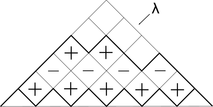
Figure 1: Definition of $n_{\lambda}$ as the sum of signed boxes. The first row of boxes is labelled with plus signs, the next with minus signs, and so on.

We will prove a more general result than (8) in Theorem 2, see Section 3.2.

3 Deformations

Let us take a pair of vectors, $w\in\mathbb{N}^{2n}$ and $\langle w\rangle\in\mathbb{C}^{2n}$, called spectral vector, satisfying the property that, for each $i$ such that $w_{i}<w_{i+1}$, then $\langle w\rangle_{i+1}\neq\langle w\rangle_{i}$ and $\langle s_{i}w\rangle=s_{i}\langle w\rangle$, where $s_{i}$ is a simple transposition. From a starting polynomial $M_{w_{0}}$ in $z_{1},\ldots,z_{2n}$, one generates other polynomials by the recursion

$$M_{w}\rightarrow M_{s_{i}w}:=T_{i}\big{(}\langle w\rangle_{i+1}-\langle w\rangle_{i}\big{)}M_{v}.$$

Thanks to the Yang-Baxter equation (2), the polynomials $M_{w^{\prime}}$ are independent of the choice of the reduced decomposition chosen to pass from $w$ to $w^{\prime}$.

Let us now be more specific and take

$$w_{0}=(n-1,\ldots,0,n-1,\ldots,0),\qquad\langle w_{0}\rangle=(n-1,n-2-u_{1},n-3-u_{2},\cdots,-u_{n-1},n-1,n-2,\ldots,2,1,0).$$

As we did in the case of KL polynomials, let us rather use partitions for indexing.

The starting point is $M_{\emptyset}=M_{w_{0}}=\Delta\Delta=\Delta_{t}(z_{1},\ldots,z_{n})\Delta_{t}(z_{n+1},\ldots,z_{2n})$. The rule to obtain the other Macdonald polynomials, which is equivalent to the description in terms of spectral vectors given in [24], is as follows. Given an arbitrary partition $\lambda=(\lambda_{n-1},\ldots,\lambda_{1})$ with $\lambda_{n-1}\geq\lambda_{n-2}\geq\ldots\geq\lambda_{1}$, the label of box $(ij)$ of the corresponding diagram is equal to $u_{n-i}+n-i-j+1$, for example,

$$M_{(\lambda_{n-1},\ldots,\lambda_{1})}(u_{1},\ldots,u_{n-1})=\;\raisebox{-120.0pt}{ \begin{picture}(220.0,220.0) \put(0.0,105.0){\begin{tabular}[]{|S|*{\value{sqcolumns}}{Z|}}\hline\cr 14.08334pt]{0.0pt}{6.83331pt}\parbox{30.0pt}{$\scriptstyle u_{n-1}+$ \\ \mbox{} \hskip 10.0pt $\scriptstyle n-1$}\@add@centering&\parbox{30.0pt}{$\scriptstyle u_{n-1}+$ \\ \mbox{} \hskip 10.0pt $\scriptstyle n-2$}\@add@centering&\ldots\@add@centering&\ldots\@add@centering&\ldots\@add@centering&$\scriptstyle u_{n-1}+1$\@add@centering\\ \hline\cr 14.08334pt]{0.0pt}{6.83331pt}\vdots\@add@centering&\@add@centering&\@add@centering&\@add@centering&\@add@centering\cr\cline{1-5}\cr 14.08334pt]{0.0pt}{6.83331pt}\vdots\@add@centering&\@add@centering&\@add@centering&\@add@centering\cr\cline{1-4}\cr 14.08334pt]{0.0pt}{6.83331pt}\vdots\@add@centering&\@add@centering&\@add@centering\cr\cline{1-3}\cr 14.08334pt]{0.0pt}{6.83331pt}$\scriptstyle u_{2}+2$\@add@centering&$\scriptstyle u_{2}+1$\@add@centering\cr\cline{1-2}\cr 14.08334pt]{0.0pt}{6.83331pt}$\scriptstyle u_{1}+1$\@add@centering\cr\cline{1-1}\cr\end{tabular}} \put(0.0,72.0){\line(1,0){36.0}} \put(35.0,72.0){\line(0,1){71.0}} \put(35.0,142.0){\line(1,0){72.0}} \put(106.0,142.0){\line(0,1){37.0}} \put(106.0,178.0){\line(1,0){36.0}} \put(142.0,177.0){\line(0,1){36.9}} \put(142.0,213.0){\line(-1,0){143.0}} \put(0.0,213.0){\line(0,-1){142.0}} \end{picture}}$$

where we have suppressed the dependence on $z_{1},\ldots,z_{2n}$. The undeformed Macdonald polynomials are obtained by setting $u_{i}=1$.

Example 4.

The deformed maximal Macdonald polynomial (for $n=3$, $q=t^{6}$) is given by

$${\rm M}_{(2,1)}(u_{1},u_{2})={\rm M}_{221100}(u_{1},u_{2})=\begin{tabular}[]{|S|*{\value{sqcolumns}}{Z|}}\hline\cr 7.58334pt]{0.0pt}{6.83331pt}$\scriptstyle u_{2}+2$\@add@centering&$\scriptstyle u_{2}+1$\@add@centering\\ \hline\cr 7.58334pt]{0.0pt}{6.83331pt}$\scriptstyle u_{1}+1$\@add@centering\cr\cline{1-1}\cr\end{tabular}\ =T_{2}(u_{1}+1)T_{4}(u_{2}+1)T_{3}(u_{2}+2)\ M_{210210}.$$

3.1 Integral formulas

Introducing an auxiliary variable $w$, we can separate the variables $z_{i}$ and $z_{i+1}$ and note the following

$$T_{i}(1)\frac{\Delta_{t}(z_{i},z_{i+1})}{(w-z_{i})(tw-t^{-1}z_{i+1})}=\\ \ \Delta_{t}(z_{i},z_{i+1})\left(\frac{1}{(w-z_{i})(w-z_{i+1})}+\frac{1}{(tw-t^{-1}z_{i})(tw-t^{-1}z_{i+1})}\right).$$ (9)

This observation naturally leads to integral formulas using Bethe Ansatz functions, see e.g. [27] for similar formulas in the context of solutions to the $q$-deformed Knizhnik-Zamolodchikov equations. First we define

$$\phi_{i}(w)=\prod_{m=1}^{i}\frac{1}{w-z_{m}}\prod_{m=i+1}^{2n}\frac{1}{tw-t^{-1}z_{m}},$$ (10)

and introduce the shift operator $S_{i}$ which acts as

$$S_{i}\phi_{i}=\phi_{i-1},\qquad S_{i}\phi_{j}=\phi_{j}\quad(j\neq i).$$ (11)

Using (9), we have the following simple action,

$$T_{i}(v_{k}+1)\Delta_{t}(z_{1},\ldots,z_{N})\phi_{i}(w) =\Delta_{t}(z_{1},\ldots,z_{N})\Big{(}S_{i}+S_{i+1}^{-1}+y_{k}\Big{)}\phi_{i}(w),$$

$$T_{i}(v_{k}+1)\Delta_{t}(z_{1},\ldots,z_{N})\phi_{j}(w) =\frac{[2+v_{k}]}{[1+v_{k}]}\Delta_{t}(z_{1},\ldots,z_{N})\phi_{j}(w)\qquad(j\neq i),$$

where

$$y_{k}=-\frac{[v_{k}]}{[v_{k}+1]}.$$

The action of the Hecke generators on the “wave functions” $\phi_{i}$ leads to the following result, in which the deformed M polynomials are explicitly given as multiple integrals.

Theorem 1.

Set $\lambda_{0}=u_{0}=0$, and let $a_{k}=\lambda_{k}+k+1$ for $0\leq k\leq n-1$. Let furthermore $y_{k}=-\frac{[v_{k}]}{[v_{k}+1]}$ where $v_{k}=u_{k}+k-\lambda_{k}$. We have

$${\rm M}_{(\lambda_{n-1},\ldots,\lambda_{1})}(u_{1},\ldots,u_{n-1})$$

$$\hphantom{{\rm M}_{(\lambda_{n-1},\ldots,\lambda_{1})}}=\Delta_{t}(z_{1},\ldots,z_{2n})\oint\cdots\oint\frac{1}{(2\pi{\rm i})^{n}}\Delta(w_{n},\ldots,w_{1})\Delta_{t}(w_{1},\ldots,w_{n})\times$$

$$\hphantom{{\rm M}_{(\lambda_{n-1},\ldots,\lambda_{1})}\Delta_{t}(z_{1},\ldots,z_{2n})}\prod_{m=0}^{n-1}\left(1+y_{m}S_{a_{m}}\right)\ \phi_{a_{m}}(w_{m+1})\hskip 2.84526pt{\rm d}w_{1}\ldots{\rm d}w_{n}$$

$$\hphantom{{\rm M}_{(\lambda_{n-1},\ldots,\lambda_{1})}}=\Delta_{t}(z_{1},\ldots,z_{2n})\oint\cdots\oint\frac{1}{(2\pi{\rm i})^{n}}\ \Delta(w_{n},\ldots,w_{1})\Delta_{t}(w_{1},\ldots,w_{n})\times$$

$$\hphantom{{\rm M}_{(\lambda_{n-1},\ldots,\lambda_{1})}\Delta_{t}(z_{1},\ldots,z_{2n})}\prod_{m=0}^{n-1}\frac{1}{[v_{m}+1]}\left(\frac{t^{v_{m}+1}w_{m+1}-t^{-v_{m}-1}z_{a_{m}}}{tw_{m+1}-t^{-1}z_{a_{m}}}\right)\phi_{a_{m}}(w_{m+1})\hskip 2.84526pt{\rm d}w_{1}\ldots{\rm d}w_{n}.$$

Remark 1.

Recall that the undeformed M polynomials are obtained by setting $u_{k}=1$ for all values of $k$. If $\lambda$ is a strict partition, then the deformed M polynomials are equal to the KL polynomials when $v_{k}=0$, or in other words $u_{k}=\lambda_{k}-k$ .

Proof.

The proof is inductive and given in B. ∎

3.2 Expansion of M into KL polynomials

Having the integrals of Theorem 1 at our disposal, we now investigate the expansion of M-basis elements into the KL basis.

Theorem 2.

Let $\mu=(\mu_{n-1},\ldots,\mu_{1})=(n-1,\ldots,1)$ be the staircase partition. The deformed maximal Macdonald polynomial $M_{\mu}(u_{1},\ldots,u_{n-1})$ is equal to the sum

$$M_{\mu}(u_{1},\ldots,u_{n-1})=\sum_{\lambda\subseteq\mu}\ c_{\lambda}\ {\rm KL}_{\lambda},$$

where the coefficients $c_{\lambda}$ are monomials in $y_{1},\ldots,y_{n-1}$ of degree at most 1 in each variable, and each KL element appears in the sum. These coefficients are recursively obtained by decomposing diagrams into ribbons, using equations (13) and (14) below.

Remark 2.

Note that since $\mu_{k}=k$ we have in this case that $u_{k}=v_{k}$ and $y_{k}=-\frac{[v_{k}]}{[v_{k}+1]}=-\frac{[u_{k}]}{[u_{k}+1]}$.

Before proving this theorem, we first give an example.

Example 5 ($n=3$).

Let

$${\rm M}_{(2,1)}(u_{1},u_{2})=T_{2}(u_{1}+1)T_{4}(u_{2}+1)T_{3}(u_{2}+2)\ \Delta_{t}(z_{1},z_{2},z_{3})\Delta_{t}(z_{4},z_{5},z_{6}).$$

The integral representation for ${\rm M}_{(2,1)}(u_{1},u_{2})$ is

$${\rm M}_{(2,1)}(u_{1},u_{2}) =\Delta_{t}(z_{1},\ldots,z_{6})\oint\oint\frac{1}{(2\pi{\rm i})^{3}}\Delta(w_{1},w_{2},w_{3})\Delta_{t}(w_{1},w_{2},w_{3})\phi_{1}(w_{1})\times$$

$$\hphantom{\Delta_{t}(z_{1},\ldots,z_{N})}\left(1+y_{1}S_{3}\right)\ \left(1+y_{2}S_{5}\right)\cdot\phi_{3}(w_{2})\phi_{5}(w_{3})\hskip 2.84526pt{\rm d}w_{1}{\rm d}w_{2}{\rm d}w_{3},$$

from which it immediately follows that

$${\rm M}_{(2,1)}(u_{1},u_{2}) ={\rm M}_{(2,1)}(0,0)+y_{1}{\rm M}_{(2)}(\cdot,0)+y_{2}{\rm M}_{(1,1)}(0,0)+y_{1}y_{2}{\rm M}_{(1)}(\cdot,0),$$

$$=\begin{tabular}[]{|S|*{\value{sqcolumns}}{Z|}}\hline\cr 1.58334pt]{0.0pt}{6.83331pt}$\scriptstyle 2$\@add@centering&$\scriptstyle 1$\@add@centering\\ \hline\cr 1.58334pt]{0.0pt}{6.83331pt}$\scriptstyle 1$\@add@centering\cr\cline{1-1}\cr\end{tabular}+y_{1}\begin{tabular}[]{|S|*{\value{sqcolumns}}{Z|}}\hline\cr 1.58334pt]{0.0pt}{6.83331pt}$\scriptstyle 2$\@add@centering&$\scriptstyle 1$\@add@centering\\ \hline\cr\end{tabular}+y_{2}\begin{tabular}[]{|S|*{\value{sqcolumns}}{Z|}}\hline\cr 1.58334pt]{0.0pt}{6.83331pt}$\scriptstyle 1$\@add@centering\\ \hline\cr 1.58334pt]{0.0pt}{6.83331pt}$\scriptstyle 1$\@add@centering\\ \hline\cr\end{tabular}+y_{1}y_{2}\begin{tabular}[]{|S|*{\value{sqcolumns}}{Z|}}\hline\cr 1.58334pt]{0.0pt}{6.83331pt}$\scriptstyle 1$\@add@centering\\ \hline\cr\end{tabular}$$

$$={\rm KL}_{(2,1)}+y_{1}{\rm KL}_{(2)}+y_{2}({\rm KL}_{(1,1)}+{\rm KL}_{\emptyset})+y_{1}y_{2}{\rm KL}_{(1)}.$$

Proof of Theorem 2.

The fact that the coefficients are polynomials in $y_{1},\ldots,y_{n-1}$ of degree at most 1 in each variable follows immediately from the first equality in Theorem 1. We will see below that they are in fact monomials.

We will use a recursive argument to prove that each KL element appears in the expansion. First note that the expansion of ${\rm M}_{n-1,n-2,\ldots,2,0}$ can be obtained from that of $M_{n-2,\ldots,1,0}$ by a shift of index ${\rm KL}_{\lambda}\rightarrow{\rm KL}_{\lambda+1^{n-2}}$, i.e. if

$${\rm M}_{n-2\ldots 10}=\sum_{\lambda\subseteq\mu}c_{\lambda}{\rm KL}_{\lambda},$$ (12)

then

$${\rm M}_{n-1\ldots 20}=\sum_{\lambda\subseteq\mu}c_{\lambda}{\rm KL}_{\lambda+1^{n-2}}.$$ (13)

This follows immediately by comparing the first line of Theorem 1 with and without shifted indices $\lambda_{k}\rightarrow\lambda_{k}+1$, $k=1,\ldots,n-1$.

Secondly, the polynomial ${\rm M}_{n-1\ldots 1}$ is the image of ${\rm M}_{n-1\ldots 20}$ under the action of $T_{2}(u_{1}+1)$, i.e.

$${\rm M}_{n-1\ldots 1}(u_{1},\ldots,u_{n-1})=T_{2}(u_{1}+1){\rm M}_{n-1\ldots 20}(u_{2},\ldots,u_{n-1}),$$

and we can use the known action of $T_{2}(u_{1}+1)=T_{2}(1)+y_{1}$ on the KL polynomials appearing in the expansion of ${\rm M}_{n-1\ldots 20}$. In order to explain this in terms of partitions, let us first define the notion of a Dyck ribbon.

Given a partition $\lambda$ and a diagonal touching an outer corner, a Dyck ribbon is a a strip $r_{\rm d}$ of boxes on the border of $\lambda$ from one outer corner to another, starting and ending on the chosen diagonal but never crossing it. The example in Figure 2 illustrates this notion pictorially, see also [28].

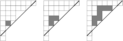
Figure 2: The partition $(7,5,3,3,2,1,1,1)$ with diagonal as shown has three Dyck ribbons.

Let $\lambda=(\lambda_{1},\ldots,\lambda_{k})$ be a partition with $k\leq n-2$, $\lambda^{\prime}$ its dual, and let $\rho$ be the staircase $(\lambda_{1}^{\prime}+1,\lambda_{1}^{\prime},\ldots,1)$. Let $R_{\rho}$ denote the set of Dyck ribbons of $\lambda$ with diagonal the diagonal of $\rho$ that runs through its corner boxes. Then the action of $T_{2}(u_{1}+1)=T_{2}(1)+y_{1}$ on ${\rm KL}_{\lambda}$ is given by [23]

$$T_{2}(u_{1}+1)\ {\rm KL}_{\lambda}=\left\{\begin{array}[]{ll}\left([2]+y_{1}\right){\rm KL}_{\lambda}=\displaystyle\frac{[u_{1}+2]}{[u_{1}+1]}{\rm KL}_{\lambda}&k<n-2\\ {\rm KL}_{\lambda,1}+y_{1}{\rm KL}_{\lambda}+\sum_{r_{\rm d}\in R_{\rho}}{\rm KL}_{\lambda-r_{\rm d}}&k=n-2,\end{array}\right.$$ (14)

where the last sum only appears if $\lambda_{n-2}=1$, and $\lambda-r_{\rm d}$ means the partition obtained by removing $r_{\rm d}$ from $\lambda$.

Example 6.

For $n=4$,

$$T_{2}(u_{1}+1){\rm KL}_{(2,2)} ={\rm KL}_{(2,2,1)}+y_{1}{\rm KL}_{(2,2)},$$

$$T_{2}(u_{1}+1){\rm KL}_{(2,1)} ={\rm KL}_{(2,1,1)}+y_{1}{\rm KL}_{(2,1)}+{\rm KL}_{(2)}+{\rm KL}_{\emptyset}.$$

Equations (13) and (14) give rise to a recursive procedure to determine the coefficients $c_{\lambda}$ in the expansion (12). A hint of how the recursion works is obtained by considering the explicit the expansion of ${\rm M}_{(3,2,1)}$ using (14), given in D.

A recursion for $c_{\lambda}$.
To complete the proof of Theorem 2,, we deduce a recursion for the coefficient $c_{\lambda}$ from (13) and (14), which is best explained in an example. We therefore show in A below how to recursively find the coefficient $c_{(2,2)}$ of ${\rm KL}_{(2,2)}$ in the expansion of ${\rm M}_{(6,5,4,3,2,1)}$. From this example it will be clear how to find the coefficient $c_{\lambda}$ for an arbitrary partition $\lambda$ in the expansion of any deformed maximal M polyomial.

The entire computation can be visualised in a single step, see Figure 3. In each iteration of the recursion, a maximal Dyck ribbon is attempted to being added to the smaller, inner, partition. This ribbon is not allowed to cross the diagonal formed by the diagonal of the staircase. In the first iteration, we fill the first maximal  Dyck ribbon with the numeral $1$ as the label of the iteration. We then consider the smaller staircase obtained by ignoring the first column. In the second iteration, the second Dyck ribbon is added, and labelled with the numeral 2. This procedure continues for the six iterations. Where no Dyck ribbon can be added, a factor of $y_{i}$ is written in the diagram. Finally, the coefficient $c_{(2,2)}$ is equal to the product of these factors, $c_{(2,2)}=y_{3}y_{5}y_{6}$.

Figure 3: Summary of the coefficient computation

The reasoning above shows, as is also clear from the explicit example in  A, that in this way one may compute the coefficient of ${\rm KL}_{\lambda}$ for any $\lambda$ in the expansion of $M_{\rho}$, with $\rho$ a staircase. The corresponding coefficient $c_{\lambda}$ is equal to the product of the factors $y_{i}$ on the diagonal, showing that this coefficient is indeed a monomial. It is also clear that each $c_{\lambda}$ is nonzero.

∎

Corollary 1.

Equation (8) holds.

Proof.

First note that the case of equation (8) corresponds to $y_{i}=\tau^{-1}=-[2]^{-1}$ for $i=1,\ldots,n$. Secondly, assigning signs as in Figure 1, the signs within each Dyck ribbon in the recursion above add up to zero. The sum over signs between inner shape and staircase is therefore the same as the number of boxes containing a factor $y_{i}$, and hence the total coefficient $c_{\lambda}$ for each inner shape $\lambda$ is equal to $c_{\lambda}=\tau^{-n_{\lambda}}$, where $n_{\lambda}$ is the total sum of signed boxes. ∎

4 Evaluations, constant term and Schubert polynomials

4.1 Evaluations

The evaluations $z_{i}=1$ of certain degenerate Macdonald and KL polynomials, normalised by dividing by the $t$-Vandermonde determinants, correspond to the number of (punctured) totally symmetric self complementary plane partitions (PTSSCPPs) with a weight in $\tau=-t-1/t$. Such enumerations were considered in [29, 14, 30, 31, 32] using methods which we will discuss in Section 3.1. Let us first give an example of two evaluations:

Example 7.

Let $\Delta\Delta=\Delta_{t}(z_{1},z_{2},z_{3})\Delta_{t}(z_{4},z_{5},z_{6})$. The ratio between the two extremal Macdonald polynomials satisfies

$$\frac{1}{\Delta\Delta}M_{221100}\Big{|}_{z_{i}=1}=3\tau^{-1}+3\tau+\tau^{3}.$$ (15)

A different result is obtained when specialising the sum of the KL basis, i.e. taking $c_{\lambda}=0$ in (8).

$$\frac{1}{\Delta\Delta}\left(KL_{111000}+KL_{110100}+KL_{101100}+KL_{110010}+KL_{101010}\right)\Big{|}_{z_{i}=1}=1+3\tau+2\tau^{2}+\tau^{3}.$$ (16)

TSSCPPs, see e.g. [33, 34, 21], are in simple bijection to nonintersecting lattice paths consisting of north and north-east steps, and starting at positions $(i,-i)$ and ending on the $x$-axis. We further augment these paths, following [14], with an extra step between the lines $y=0$ and $y=1$, in such a way that the difference of successive $x$ coordinates of the end positions are odd numbers, and the coordinate of the first endpoint is 1. We also assign a weight $\tau$ to vertical steps, and a weight $t$ to vertical augmented step.

Example 8.

The seven weighted paths for $n=2$ are

The weighted enumeration of these augmented paths is $N(t,\tau)=\tau^{3}+2t\tau^{2}+2t^{2}\tau+\tau+t$.

Note that for special values of $t$ we obtain the evaluations in Example 7.

$$N(\tau^{-1},\tau)=3\tau^{-1}+3\tau+\tau^{3},\qquad N(1,\tau)=1+3\tau+2\tau^{2}+\tau^{3}.$$

In the next section we clarify this correspondence and give a unified description of the M and KL polynomials.

4.2 Constant term

In this section we further investigate the homogeneous limit $z_{i}\rightarrow 1$. The following change of variables is useful

$$z_{i}=\frac{1-t^{-1}\zeta_{i}}{1-t\zeta_{i}},\qquad w_{i}=\frac{1-t^{-1}x_{i}}{1-tx_{i}}.$$ (17)

We also define

$$\tau=-(t+t^{-1}).$$

Proposition 1 (Homogenous limit).

In the homogeneous limit $\zeta_{i}\rightarrow 0$ we obtain

$${\rm M}_{\lambda_{n-1},\ldots,\lambda_{1}}(u_{1},\ldots,u_{n-1})=\\ (t-t^{-1})^{n(n-1)}\oint\cdots\oint\prod_{m=0}^{n-1}\frac{{\rm d}x_{m+1}\ (1+y_{m}x_{m+1})}{2\pi{\rm i}\ x_{m+1}^{a_{m}}}\prod_{1\leq i<j\leq n}(x_{j}-x_{i})(1+x_{i}x_{j}+\tau x_{j}),$$

where we recall that $a_{k}=\lambda_{k}+k+1$ and $y_{k}=-\frac{[v_{k}]}{[v_{k}+1]},\ v_{k}=u_{k}+k-\lambda_{k}$ and $y_{0}=0$.

A proof or Proposition 1 is given in C.

The contour integrals in Proposition 1 pick out the residues around zero of each variable $x_{i}$. The integral can be rewritten as the following constant term expression

$$A_{a_{1},\ldots,a_{n-1}}(\tau,y_{1},\ldots,y_{n-1})=\operatorname{CT}\left(\prod_{i=0}^{n-1}(1+y_{i}x_{i+1})x_{i+1}^{-a_{i}+1}\prod_{i<j}(x_{j}-x_{i})(1+x_{i}x_{j}+\tau x_{j})\right),$$ (18)

where $\operatorname{CT}=$ constant term with respect to each variable $x_{i}$. In the case $a_{i}=2i+1$ for $i=0,\ldots,n-1$ and $y_{1}=\ldots=y_{n-1}=y$, expression (18) is equal to a constant term expression given by Di Francesco and Zinn-Justin in [14]. In the same paper, a formula (Formula 2.7) is given for the number of TSSCPPs according to the heights of the vertical steps. This formula reads

$$N(t_{0},\dots,t_{n-1})=\operatorname{CT}\left(\prod_{i<j}\frac{(x_{j}-x_{i})(1+t_{i}x_{j})}{1-x_{i}x_{j}}\prod_{i}\frac{1+t_{0}x_{i}}{1-x_{i}^{2}}\prod_{i=1}^{n}x_{i}^{-2i+2}\right)$$ (19)

When $t_{1}=\ldots t_{n-1}=\tau$, the two constant terms (18) and (19) are equal:

Theorem 3 (Zeilberger-Di Francesco-Zinn Justin).

$$N(t,\tau,\ldots,\tau)=A_{1,3,\ldots,2n-1}(\tau,t,\ldots,t).$$

Proof.

This can be shown by symmetrising the argument of the constant term (18) with respect to the variables $x_{i}$, [14, 35]. ∎

We have not been able to establish a relation between $N$ and $A$ for general values of $y_{i}$ and $t_{i}$. Fonseca and Zinn-Justin[31], and Fonseca and Nadeau [32] consider the number of punctured totally symmetric self complementary plane partition with a puncture of size $r$. Their generation function is equal to

$$N_{n,r}(\tau)=\operatorname{CT}\left(\prod_{i<j}\frac{(x_{j}-x_{i})(1+\tau x_{j})}{1-x_{i}x_{j}}\prod_{i}\frac{(1+x_{i})(1+\tau x_{i})^{r}}{1-x_{i}^{2}}\prod_{i=1}^{n}x_{i}^{-2i+2}\right)$$

Theorem 4.

Let $\mu^{(r)}=(\mu^{(r)}_{n-1},\ldots,\mu^{(r)}_{1})$ be the staircase partition $(n-r-1,n-r-2,1,0,\ldots,0)$. Then we have

$$N_{n-r,r}(\tau)=M_{\mu^{(r)}}(u_{i}=1-r;z_{i}=1)=A_{123\cdots,r-1,r+1,r+3,\ldots 2n-r-1}(\tau,1,\ldots,1).$$

Example 9.

For $n=5$ and $r=2$ we have $\mu_{2}=(2,1,0,0)$ and

$$N_{3,2}(\tau)=M_{(2,1,0,0)}(u_{1}=\cdots=u_{4}=-1)=A_{12357}(\tau,1,1,1,1,1)=1+7\tau+12\tau^{2}+14\tau^{3}.$$

4.3 Schubert polynomials

Schubert polynomials are a linear basis of the ring of polynomials. Though having been introduced in relation with Schubert calculus on flag varieties, they will be specially appropriate for the computation of the functions $N(t_{0},\dots,t_{n-1})$. Let us recall some facts about these polynomials (see e.g. [36]).

Let $n$ be an integer, $\mathbf{x}=\{x_{1},\ldots,x_{n}\}$, $\mathbf{y}=\{y_{1},y_{2},\ldots,y_{\infty}\}$. The Schubert polynomials $Y_{v}(\mathbf{x},\mathbf{y})$, $v\in\mathbb{N}^{n}$, are a linear basis of the space of polynomials in $\mathbf{x}$ with coefficients in $\mathbf{y}$. They are recursively defined starting from the case where $v$ is dominant, i.e. $v=\lambda=\lambda_{1}\ldots\lambda_{n}$, $\lambda_{1}\geq\lambda_{2}\ldots\geq\lambda_{n}\geq 0$ (we also say that $\lambda$ is a partition). In that case

$$Y_{\lambda}(\mathbf{x},\mathbf{y}):=\prod_{i=1}^{n}\prod_{j=1}^{\lambda_{i}}(x_{i}-y_{j})\,.$$

The general polynomials are then defined by

$$\partial_{i}Y_{v}(\mathbf{x},\mathbf{y})=Y_{[\ldots,v_{i-1},v_{i+1},v_{i}-1,v_{i+2},\ldots]}(\mathbf{x},\mathbf{y})\ ,\ v_{i}>v_{i+1}\,,$$ (20)

(in the case where $v_{i}\leq v_{i+1}$, then $\partial_{i}Y_{v}(\mathbf{x},\mathbf{y})=0$ since $\partial_{i}\partial_{i}=0$).

One can also index Schubert polynomials by permutations , the code of a permutation [36, 37]) furnishing the correspondence between the two indexings.

Since the image of $\partial_{i}$ is the space of polynomials which are symmetric in $x_{i},x_{i+1}$, the Schubert polynomial $Y_{v}(\mathbf{x},\mathbf{y})$ has this symmetry whenever $v_{i}\leq v_{i+1}$. In particular, if $v$ is such that $v_{1}\leq\cdots\leq v_{n}$, then $Y_{v}(\mathbf{x},\mathbf{y})$ is symmetric in $x_{1},\ldots,x_{n}$ and is called a Graßmannian Schubert polynomial. It specializes to the Schur function in $\mathbf{x}$ indexed by the partition $v_{n}\ldots v_{1}$ for $\mathbf{y}={\mathbf{0}}=\{0,0,\ldots\}$.

Example 10.

A dominant Schubert polynomial can be visualised on the diagram corresponding to the index of the polynomial. Each box is filled with a factor of the form $(x_{i}-y_{j})$, placed in the $i$th row and $j$th column. The Schubert polynomial is equal to the product of these factors. For $v=421$ the diagram is

so that we have

$$Y_{[4,2,1]} = (x_{1}-y_{1})(x_{1}-y_{2})(x_{1}-y_{3})(x_{1}-y_{4})(x_{2}-y_{1})(x_{2}-y_{2})(x_{3}-y_{1}).$$

Following these preliminaries on Schubert polynomials, we now state

Theorem 5.

Let $n$ be an integer, $\rho=n-1,\ldots,1$. For any $\lambda\subseteq\rho$, let $\mu=\lambda^{\prime}$ be the conjugate partition, and let $(\rho/\lambda)=0,n-1-\mu_{1},0,n-2-\mu_{2},0,n-3-\mu_{3},0,\dots$.

Then the constant term (19) is equal to

$$N(t_{0},\dots,t_{n-1})=\sum_{\lambda\subseteq\rho,\hskip 2.84526pt\lambda\mbox{ {\small\it even}}}Y_{(\rho/\lambda)}({\bf\bar{y}},0),$$ (22)

and the alphabet ${\bf\bar{y}}$ being specialized into $\{t_{0},t_{1},0,t_{2},0,t_{3},0,\dots\}$.

Proof of Theorem 5.

Let us analyse the expression (19). One first extracts the kernel $\prod_{i<j}(1-x_{i}/x_{j})$, then the symmetric function $\prod_{i\leq j}(1-x_{i}x_{j})^{-1}$. What remains can be identified with a Schubert polynomial. This allows us to use the following fundamental scalar product on polynomials: given two polynomials, $f$, $g$, one defines

$$\langle f,g\rangle=\operatorname{CT}\left(f(x_{1},\dots,x_{n})g(x_{n}^{-1},\dots,x_{1}^{-1})\prod_{1\leq i<j\leq n}(1-\frac{x_{i}}{x_{j}})\right).$$ (23)

It is proved in [38] that this scalar product coincides with the usual scalar product when restricted to symmetric functions. The function $N(t_{0},\dots,t_{n-1})$ is now written

$$N(t_{0},\dots,t_{n-1}) = \operatorname{CT}\left(\prod_{i<j}(1-\frac{x_{i}}{x_{j}})\prod_{i\leq j}(1-x_{i}x_{j})^{-1}\prod_{i<j}(1+t_{i}x_{j})\prod_{i=1}^{n}(1+t_{0}x_{i})\prod_{i=1}^{n}x_{i}^{-i+1}\right)$$ (24)

$$= \left\langle\prod_{i\leq j}(1-x_{i}x_{j})^{-1},\prod_{i<j}(1+\frac{t_{i}}{x_{n+1-j}})\prod_{i=1}^{n}(1+\frac{t_{0}}{x_{i}})x^{\rho_{i}}\right\rangle$$

$$= \left\langle\prod_{i\leq j}(1-x_{i}x_{j})^{-1},\prod_{i+j\leq n}(x_{i}+t_{j})\prod_{i=1}^{n-1}(1+\frac{t_{0}}{x_{i}})\right\rangle$$

as the term $t_{0}/x_{n}$ does not contribute to the constant term.

Define the operator $\partial_{\omega}$ by taking a reduced decomposition $s_{i}\dots s_{k}$ of the permutation $(n,\dots,1)$ and putting $\partial_{i}\dots\partial_{k}=\partial_{\omega}$. Recall that the operator $\pi_{\omega}:\ f\mapsto\partial_{\omega}(x^{\rho}f)$ is self adjoint and sends a dominant monomial $x^{\lambda}$ onto the Schur function of the same index. Since the LHS of the scalar product is symmetric, one can symmetrize the RHS under $\pi_{\omega}$, transforming it into

$$\partial_{w}\left(\prod_{i+j\leq n}(x_{i}+t_{j})\prod_{i=1}^{n-1}(1+\frac{t_{0}}{x_{i}})x_{i}^{\rho_{i}}\right).$$ (25)

However

$$\prod_{i+j\leq n}(x_{i}+t_{j})\prod_{i}^{n-1}(1+\frac{t_{0}}{x_{i}})x_{i}^{\rho_{i}}$$

is equal to the dominant Schubert polynomial of index $[2n-2,2n-4,\dots,2,0]$ for the alphabets ${\bf x}=\{x_{1},\dots,x_{n}\}$, ${\bf y}=\{-t_{0},-t_{1},0,-t_{2},0,-t_{3},\dots\}$. For example, for $n=4$, this Schubert polynomial is

We can therefore write

$$N(t_{0},\dots,t_{n-1}) = \left\langle\prod_{i\leq j}(1-x_{i}x_{j})^{-1},\partial_{\omega}Y_{[2n-2,2n-4,\dots,2,0]}({\bf x},{\bf y})\right\rangle.$$ (27)

Using $\partial_{\omega}=\partial_{n-1}\circ\partial_{n-2}\partial_{n-1}\circ\dots\circ\partial_{2}\partial_{3}\dots\partial_{n-2}\partial_{n-1}$ and (20), we can simplify the RHS of the scalar product with

$$\partial_{\omega}Y_{[2n-2,2n-4,\dots,2,0]}({\bf x},{\bf y})=Y_{[0,1,\ldots,n-1]}({\bf x},{\bf y}).$$

There is a Cauchy formula for Schubert polynomials [36, (Theorem 10.2.6)], which decomposes a Schubert polynomial into an alternating sum of products of Schubert polynomials in each of the alphabets ${\bf x}$, ${\bf y}$ separately. In our case, $Y_{[0,1,...,n-1]}({\bf x},{\bf y})$ is symmetric in $x_{1},\dots,x_{n}$ and decomposes into a sum of Schur functions in ${\bf x}$:

$$Y_{[0,1,2,\dots,n-1]}({\bf x},{\bf y})=\sum_{\lambda\subseteq\rho}S_{\lambda}({\bf x})Y_{(\rho/\lambda)}({\bf\bar{y}},0),$$ (28)

the definition of the index $(\rho/\lambda)$ and the alphabet ${\bf\bar{y}}$ being given in the statement of the theorem.

The LHS of the scalar product is equal to the sum of all Schur functions indexed by an even partition (i.e. with even parts). Therefore, the scalar product is equal to

$$N(t_{0},\dots,t_{n-1})=\sum_{\lambda\subseteq\rho,\hskip 2.84526pt\lambda\mbox{ {\small even}}}Y_{(\rho/\lambda)}({\bf\bar{y}},0).$$

∎

Example 11.

For $n=3$, we have $\rho=21$. The two possible even sub-partitions are $\lambda=\emptyset$ and $\lambda=2$. The two conjugate partitions are $\mu=\lambda^{\prime}=\emptyset$, and $\mu=\lambda^{\prime}=11$ respectively. Considering the first of these we have

$$(\rho/\lambda)=(21/0)=[0,n-1-\mu_{1},0,n-2-\mu_{2},0]=[0,2,0,1,0],$$

and for the second sub-partition we have

$$(\rho/\lambda)=(21/2)=[0,n-1-\mu_{1},0,n-2-\mu_{2},0]=[0,1,0,0,0].$$

Thus the two polynomials contributing to the constant term $N(t_{0},t_{1},t_{2})$ are

$$Y_{[0,2,0,1,0]}({\bf\bar{y}},0)\mbox{ and }Y_{[0,1,0,0,0]}({\bf\bar{y}},0)$$

4.4 Determinant expression

The Schubert polynomials in Theorem 5 have a determinantal expression that we are now going to introduce. The complete symmetric function of degree $k$ is defined to be the sum of all monomials of total degree $k$ – see e.g. [39]. Let $h_{k}(r)$ denote the complete symmetric function of degree $k$ in the alphabet ${\bf\bar{y}}=\{y_{1},\dots,y_{2r-2}\}=\{t_{0},t_{1},0,t_{2},0,t_{3},\dots,t_{r-1}\}$. We also use the notation $\mu=\lambda^{\prime}$.

The indices of the Schubert polynomials in ${\bf\bar{y}}$ on the RHS of (22), are all codes which can be obtained from an increasing partition under the Schubert recursion (20). Therefore, these polynomials are all images of Schur functions in ${\bf\bar{y}}$ under divided differences.

Schur functions have a determinantal expression in terms of complete functions (Jacobi-Trudi determinants). We need to generalize these determinants by allowing flags of alphabets. Given two partitions $\rho,\lambda$, an alphabet ${\bf\bar{y}}=\{y_{1},y_{2},\dots\}$, an increasing sequence of positive integers $\Phi=(\phi_{1},\phi_{2},\dots)$, then the flag Schur function $S_{\rho/\lambda}({\mathbf{\bar{y}}},\Phi)$ is equal to

$$S_{\rho/\lambda}({\mathbf{\bar{y}}},\Phi)=\det\left(h_{\rho_{i}-\mu_{j}-i+j}({\phi_{i}})\right)_{i,j=1\dots n-1}.$$

The action of divided differences on such determinants, under some hypotheses which are satisfied in our case, is easy, see e.g. [36, Lemma 1.4.5] or [37, Corollary 2.6.10]. At each step any divided difference acts on a single row only (or on no row). From (20) it follows that this action consists in decreasing the indices of the complete symmetric functions in this row and transforming their argument $r$ into $r+1$. We thus obtain

Proposition 2.

Let $\mu=\lambda^{\prime}$ be the partition conjugate to $\lambda$. Then

$$Y_{(\rho/\lambda)}({\bf\bar{y}},0)=S_{\rho/\lambda}({\mathbf{\bar{y}}},\Phi)$$ (29)

where $\Phi=(2,4,\dots,2n-2)$. Equivalently, suppressing the 0’s in ${\bf\bar{y}}$ and using the alphabet ${\bf\tilde{y}}=(t_{0},t_{1},t_{2},t_{3},\ldots)$ with $\tilde{h}_{i}(r)$ the complete symmetric function in the alphabet ${\bf\tilde{y}}$, one has

$$Y_{(\rho/\lambda)}({\bf\tilde{y}},0)=S_{\rho/\lambda}({\bf\tilde{y}},{\widetilde{\Phi}})=\det\left(\tilde{h}_{\rho_{i}-\mu_{j}-i+j}({\tilde{\phi}_{i}})\right)_{i,j=1\dots n-1}$$ (30)

where the flag is equal to $\widetilde{\Phi}=(2,3,\ldots,n)$.

We illustrate this is in the following examples.

Example 12.

$$Y_{[4,6,7]}({\bf\bar{y}},0)=\begin{vmatrix}h_{4}(1)&h_{7}(1)&h_{9}(1)\\ h_{3}(2)&h_{6}(2)&h_{8}(2)\\ h_{2}(3)&h_{5}(3)&h_{7}(3)\end{vmatrix}.$$

We transform this into $Y_{[0,3,0,4,0,4]}$ using the sequence of divided difference operators $\partial_{1}\partial_{3}\partial_{2}\partial_{5}\partial_{4}\partial_{3}$. The first step gives

$$Y_{[4,6,7]}\stackrel{{\scriptstyle\partial_{3}}}{{\to}}Y_{[4,6,0,6]}=\begin{vmatrix}h_{4}(1)&h_{7}(1)&h_{9}(1)\\ h_{3}(2)&h_{6}(2)&h_{8}(2)\\ h_{1}(4)&h_{4}(4)&h_{6}(4)\end{vmatrix},$$

and the remaining transformations lead to

$$Y_{[4,6,0,6]}\stackrel{{\scriptstyle\partial_{4}}}{{\to}}Y_{[4,6,0,0,5]}\stackrel{{\scriptstyle\partial_{5}}}{{\to}}Y_{[4,6,0,0,0,4]}\stackrel{{\scriptstyle\partial_{2}}}{{\to}}Y_{[4,0,5,0,0,4]}\stackrel{{\scriptstyle\partial_{3}}}{{\to}}Y_{[4,0,0,4,0,4]}\stackrel{{\scriptstyle\partial_{1}}}{{\to}}Y_{[0,3,0,4,0,4]}=\begin{vmatrix}h_{3}(2)&h_{6}(2)&h_{8}(2)\\ h_{1}(4)&h_{4}(4)&h_{6}(4)\\ 0&h_{2}(6)&h_{4}(6)\end{vmatrix}.$$

Recall that we have taken the alphabet ${\bf\bar{y}}=(t_{0},t_{1},0,t_{2},\ldots)$, and the flag consists of exactly the positions of the non-zero components of the index. Then

$$Y_{[0,3,0,4,0,4]}=\begin{vmatrix}\tilde{h}_{3}(2)&\tilde{h}_{6}(2)&\tilde{h}_{8}(2)\\ \tilde{h}_{1}(3)&\tilde{h}_{4}(3)&\tilde{h}_{6}(3)\\ 0&\tilde{h}_{2}(4)&\tilde{h}_{4}(4)\end{vmatrix}.$$

Example 13.

Using (30), we write

$$Y_{[0,2,0,1,0]}({\bf\bar{y}},0) = \left|\begin{matrix}h_{2}(2)&h_{3}(2)\\ h_{0}(3)&h_{1}(3)\end{matrix}\right|$$

$$= \left|\begin{matrix}(t_{0}^{2}+t_{0}t_{1}+t_{1}^{2})&(t_{0}^{3}+t_{0}^{2}t_{1}+t_{0}t_{1}^{2}+t_{1}^{3})\\ 1&(t_{1}+t_{1}+t_{2})\end{matrix}\right|$$

$$= t_{0}^{2}t_{1}+t_{0}^{2}t_{2}+t_{0}t_{1}^{2}+t_{0}t_{1}t_{2}+t_{1}^{2}t_{2}.$$

Similarly

$$Y_{[0,1,0,0,0]}({\bf\bar{y}},0) = \left|\begin{matrix}h_{1}(2)&h_{2}(2)\\ h_{-1}(3)&h_{0}(3)\end{matrix}\right|$$

$$= \left|\begin{matrix}(t_{0}+t_{1})&(t_{0}^{2}+t_{0}t_{1}+t_{1}^{2})\\ 0&1\end{matrix}\right|$$

$$= t_{0}+t_{1}.$$

and thus

$$N(t_{0},t_{1},t_{2})=Y_{[0,2,0,1,0]}({\bf\bar{y}},0)+Y_{[0,1,0,0,0]}({\bf\bar{y}},0)=t_{0}+t_{1}+t_{0}^{2}t_{1}+t_{0}^{2}t_{2}+t_{0}t_{1}^{2}+t_{0}t_{1}t_{2}+t_{1}^{2}t_{2}.$$ (31)

4.5 Combinatorial interpretation

Having interpreted the constant term in terms of Schubert polynomials, one gets for free a combinatorial interpretation in terms of tableaux. Indeed, $Y_{[0,n-1,0,\dots,3,0,2,0,1]}({\bf\bar{y}})$ is equal to a sum of semi-standard tableaux of staircase shape, that we represent in the French way in the Cartesian plane, satisfying a flag condition. Taking the alphabet ${\bf\tilde{y}}=(t_{0},t_{1},t_{2},t_{3},\dots)$, the Schubert polynomial becomes $Y_{[0,n-1,n-2,\dots,2,1]}({\bf\tilde{y}})$, which can be interpreted as the sum of tableaux of staircase shape such that the bottom row belongs to $\{1,2\}^{*}$, i.e only $t_{0}$ and $t_{1}$ can be used as fillings for this row, the next one to $\{1,2,3\}^{*},\dots,$ the top one to $\{1,\dots,n\}^{*}$. We say that such a tableau satisfies the flag condition $2,3,\dots,n$. For $n=4$, this is

$$\begin{array}[]{ll}\raisebox{-14.22636pt}{ \begin{tabular}[]{|S|*{\value{sqcolumns}}{Z|}}\cline{1-1}\cr 9.08336pt]{0.0pt}{6.83331pt}\@add@centering\cr\cline{1-2}\cr 9.08336pt]{0.0pt}{6.83331pt}\@add@centering&\@add@centering\cr\cline{1-3}\cr 9.08336pt]{0.0pt}{6.83331pt}\@add@centering&\@add@centering&\@add@centering\\ \cline{1-3}\cr\end{tabular}}&\begin{array}[]{l}{\rm flag}\\[9.95845pt] 4\\[14.22636pt] 3\\[14.22636pt] 2\end{array}\end{array}$$

This interpretation remains valid for skew shapes. As usual in the theory of tableaux, this result is obtained by introducing an extra alphabet of small letters, which fill the inner shape. The valuation of these tableaux for a fixed inner shape with even columns are exactly the determinants written above.
Therefore, (22) becomes

Theorem 6.

The constant term $N(t_{0},\dots,t_{n-1})$ is the commutative image of the sum of tableaux of outer shape $\rho=n-1,\dots,1$, inner shape with columns of even lengths, satisfying the flag condition $2,3,\dots,n$.

In fact, one can reprove directly that the generating function $N(t_{0},\dots,t_{n-1})$ is given by a sum of tableaux.

Example 14.

For $n=3$, the sum

$$Y_{(21/0)}({\bf\bar{y}},0)+Y_{(21/2)}({\bf\bar{y}},0)=Y_{[0,2,0,1,0]}({\bf\bar{y}},0)+Y_{[0,1,0,0,0]}({\bf\bar{y}},0)$$

is given by the tableaux

and this agrees with

$$N(t_{0},t_{1},t_{2})=t_{0}^{2}t_{2}+t_{0}t_{1}t_{2}+t_{1}^{2}t_{2}+t_{0}^{2}t_{1}+t_{0}t_{1}^{2}+t_{0}+t_{1}.$$

We now introduce another object which is in bijection with TSSCPP. We take the staircase shape now in the north-west corner (here for $n=5$):

$$\Box\hskip 14.22636pt\Box\hskip 14.22636pt\Box\hskip 14.22636pt\Box$$

$$\Box\hskip 14.22636pt\Box\hskip 14.22636pt\Box$$

$$\Box\hskip 14.22636pt\Box$$

$$\Box$$

with border:

$$\Box\hskip 14.22636pt\Box\hskip 14.22636pt\Box\hskip 14.22636pt\Box\hskip 12.51918pt(0)\hskip 56.9055pt$$

$$\Box\hskip 14.22636pt\Box\hskip 14.22636pt\Box\hskip 12.51918pt(1)$$

$$\Box\hskip 14.22636pt\Box\hskip 12.51918pt(2)$$

$$\Box\hskip 12.51918pt(3)$$

The TSSCPP are in bijection with the fillings of the completed staircase such that rows are weakly decreasing from left to right, and decrease by $1$ at most (taking into account the border). Each filling corresponds to a configuration of non-intersecting lattice paths, beginning at $(i,-i)$, obtained by reading each row from right to left, and an increase in the integer corresponds to a vertical step.

Example 15.

For the filling

$$\hskip 28.45274pt1\hskip 14.22636pt1\hskip 14.22636pt1\hskip 14.22636pt0\hskip 10.5275pt(0)$$

$$\hskip 28.45274pt2\hskip 14.22636pt2\hskip 14.22636pt1\hskip 10.5275pt(1)$$

$$\hskip 28.45274pt3\hskip 14.22636pt3\hskip 10.5275pt(2)$$

$$\hskip 28.45274pt3\hskip 10.5275pt(3)$$

we obtain the non-intersecting lattic paths (NILP) shown in Figure 4.

Figure 4: Non-intersecting lattice path configuration. Reading each row from right to left, an increase in value corresponds to a vertical step

Now add a left column (column $0$) as follows. If the number of rows is even (resp. odd), then it consists of the even (resp. odd) numbers immediately bigger than or equal to the numbers in the first column. For example,

$$\begin{array}[]{ccc}\begin{array}[]{lllll}\hskip 28.45274pt1\hskip 14.22636pt1\hskip 14.22636pt1\hskip 14.22636pt0\hskip 10.5275pt(0)\\ \hskip 28.45274pt2\hskip 14.22636pt2\hskip 14.22636pt1\hskip 10.5275pt(1)\\ \hskip 28.45274pt3\hskip 14.22636pt3\hskip 10.5275pt(2)\\ \hskip 28.45274pt3\hskip 10.5275pt(3)\end{array}&{\rm becomes}&\begin{array}[]{lllll}2\hskip 14.22636pt1\hskip 14.22636pt1\hskip 14.22636pt1\hskip 14.22636pt0\hskip 10.5275pt(0)\\ 2\hskip 14.22636pt2\hskip 14.22636pt2\hskip 14.22636pt1\hskip 10.5275pt(1)\\ 4\hskip 14.22636pt3\hskip 14.22636pt3\hskip 10.5275pt(2)\\ 4\hskip 14.22636pt3\hskip 10.5275pt(3)\end{array}\end{array}$$

This corresponds to the completion defined by Di Francesco and Zinn-Justin in [14], and discussed in Section 4.1 (see Example 8). Again the rows describe the successive paths (read from right to left) composing the TSSCPP, an increase corresponding to a vertical step.

Example 16.

For the filling, with completion described above, we have the path configuration shown in Figure 5.

Figure 5: Augmented non-intersecting lattice path configuration. Again reading each row from right to left, and an increase in value corresponds to a vertical step

But such an object can also be read as a usual skew Young tableau (in the Cartesian plane, with strictly decreasing columns, and weakly increasing rows) of outer shape the staircase, with inner shape the diagram with lengths of columns the complement of column $0$ to $(n-1)^{n-1}$. In the example above the inner shape would be $4444-2244=2200$. One records the positions of the decreases in row $1,2,\dots,$ (reading left to right), and this gives columns $1,2,\dots$ of the tableau (reading bottom to top). Such a tableau satisfies the flag condition $2,3,\dots$, its commutative evaluation is exactly the weight of the corresponding TSSCPP (where $t_{0}$ is the weight of each augmented vertical step, $t_{1}$ the weight of each vertical step in the row immediately below this, etc.). The example becomes

and thus has a weight $t_{0}^{3}t_{2}^{2}t_{3}$.

In summary, each weighted NILP corresponds to a filling, as described above. Each filling corresponds to a skew tableau, satisfying a flag condition, describing a monomial of the Schubert polynomial $Y_{(\rho/\lambda)}({\bf\bar{y}},0)$ for some even partition $\lambda$.

Appendix A Explicit example of the recursion in the proof of Theorem 2

Consider the Macdonald polynomial ${\rm M}_{(6,5,4,3,2,1)}$, i.e. corresponding to the maximal staircase of size $n=7$. We wish to find the coefficient of ${\rm KL}_{(2,2)}$ in the expansion of this polynomial. To do so, we begin by drawing the partition $(2,2)$ inside the staircase.

Figure 6: The maximal staircase of size $n=7$, with inner shape $(2,2)$

We now show the recursion step by step.

$\bullet$ First iteration
Step 1: We draw in the diagonal bounding the staircase, and add the maximal Dyck ribbon to the inner shape (if possible). This is shown in Figure 7(a).
Step 2: The second step is to delete the first column. Our inner shape is now the remainder of $(2,2)$ and the added Dyck ribbon, i.e. the new inner shape becomes $(4,2,2)$, see Figure 7(b).

(a) The maximal Dyck ribbon is shaded

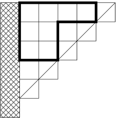
(b) The first column is removed, and new inner shape drawn

Figure 7: Steps 1 and 2 in the first iteration

$\bullet$ Second iteration
We now repeat steps 1 and 2, with the new inner shape and smaller staircase:
Step 1: We draw in the diagonal bounding the staircase, and add the maximal Dyck ribbon to $(4,4,2,2)$ inside $(5,4,3,2,1,1)$. This is shown in Figure 8(a).
Step 2: We again remove the first column, see Figure 8(b), the new inner shape is $(3,1,1)$.

(a) The maximal Dyck ribbon is just the shaded single box

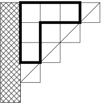
(b) The first column is again removed, and new inner shape drawn

Figure 8: Steps 1 and 2 in the second iteration

$\bullet$ Third iteration
Step 1: It is not possible to add a Dyck ribbon, see Figure 9(a). This has the consequence that now we pick up a factor of $y_{3}$.
Step 2: We again remove the first column, see Figure 9(b). The new inner shape is $(2)$.

(a) No Dyck ribbon can be added

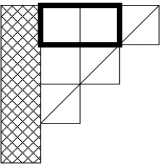
(b) The first column is again removed

Figure 9: Steps 1 and 2 in the third iteration

$\bullet$ Fourth iteration
We repeat steps 1 and 2, with the new inner shape and smaller staircase:
Step 1: We draw in the diagonal bounding the staircase, and add the maximal Dyck ribbon, see Figure 10(a).
Step 2: We again remove the first column, see Figure 10(b). The new inner shape is $(1)$.

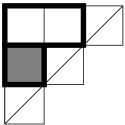
(a) Maximal Dyck ribbon

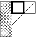
(b) First column removed

Figure 10: Steps 1 and 2 in the fourth iteration

$\bullet$ Fifth and sixth iterations
Repeating steps we see that no further Dyck ribbons can be added, see Figure 11. For these iterations therefore result in factors $y_{5}$ and $y_{6}$:

Figure 11: Steps 1 and 2 in the fifth and sixth iteration

Since we could not add Dyck ribbons at iterations 3, 5 and 6, we picked up corresponding factors $y_{3}$, $y_{5}$ and $y_{6}$. The claim is that the coefficient of $KL_{(2,2)}$ in the expansion of $M_{(6,5,4,3,2,1)}$ is just $y_{3}y_{5}y_{6}$.

Appendix B Proof of Theorem 1

B.1 One row

First we recall

$$\phi_{i}(w)=\prod_{m=1}^{i}\frac{1}{w-z_{m}}\prod_{m=i+1}^{N}\frac{1}{tw-t^{-1}z_{m}},$$ (34)

and we have

$$T_{i}(v)\Delta_{t}(z_{1},\ldots,z_{N})\phi_{i}(w) =\Delta_{t}(z_{1},\ldots,z_{N})\Big{(}\phi_{i-1}(w)+\phi_{i+1}(w)+\frac{[1-v]}{[v]}\phi_{i}(w)\Big{)},$$ (35)

$$T_{i}(v)\Delta_{t}(z_{1},\ldots,z_{N})\phi_{j}(w) =\frac{[1+v]}{[v]}\Delta_{t}(z_{1},\ldots,z_{N})\phi_{j}(w)\qquad(j\neq i).$$ (36)

We now look for a solution $\psi_{i}$ of (35) and (36) satisfying the boundary conditions $\psi_{0}=\psi_{N+1}=0$. These boundary conditions can be fixed using Cauchy’s theorem. Let $C_{0}$ denote the contour lying around all poles at $z_{i}$ ($i=1,\ldots,N$), and let $C_{1}$ be the contour lying around the poles at $t^{-2}z_{i}$. As $\phi_{i}(w){\rm d}w$ has no pole at infinity, the contour $C_{0}$ may be deformed to $C_{1}$, and we have

$$\oint_{C_{0}}\frac{1}{2\pi{\rm i}}\ \phi_{i}(w)\hskip 2.84526pt{\rm d}w=-\oint_{C_{1}}\frac{1}{2\pi{\rm i}}\ \phi_{i}(w)\hskip 2.84526pt{\rm d}w.$$ (37)

By Cauchy’s theorem, the first integral obviously gives zero for $i=0$, and second is clearly zero for $i=N$.

Let us now define

$$\psi_{i}=\Delta_{t}(z_{1},\ldots,z_{N})\oint_{C_{0}}\frac{1}{2\pi{\rm i}}\ \phi_{i}(w)\hskip 2.84526pt{\rm d}w,$$ (38)

and note that

$$\psi_{2}(v_{0}):=T_{1}(v_{0}+1)\psi_{1}=\psi_{2}-\frac{[v_{0}]}{[v_{0}+1]}\psi_{1}.$$

Let us further introduce the shift operator $S_{i}$ which acts as

$$S_{i}\phi_{i}=\phi_{i-1},\qquad S_{i}\phi_{j}=\phi_{j}\quad(j\neq i).$$ (39)

We then have that

$$\psi_{2}(v_{0}) =\Delta_{t}(z_{1},\ldots,z_{N})\oint\frac{1}{2\pi{\rm i}}\ \left(1-\frac{[v_{0}]}{[v_{0}+1]}S_{2}\right)\ \phi_{2}(w)\hskip 2.84526pt{\rm d}w$$

$$=\Delta_{t}(z_{1},\ldots,z_{N})\oint\frac{1}{2\pi{\rm i}}\ \left(\frac{1}{[v_{0}+1]}\frac{t^{v_{0}+1}w-t^{-v_{0}-1}z_{2}}{tw-t^{-1}z_{2}}\right)\phi_{2}(w)\hskip 2.84526pt{\rm d}w.$$

More generally we define

$$\psi_{a_{0}}(v_{0})=T_{a_{0}-1}(v_{0}+1)\cdots T_{1}(v_{0}+a_{0}-1)\psi_{1},$$ (40)

which we denote by

$$\psi_{a_{0}}(v_{0})=\begin{tabular}[]{|S|*{\value{sqcolumns}}{Z|}}\hline\cr 14.08336pt]{0.0pt}{6.83331pt}$\scriptstyle v_{0}+a_{0}-1$\@add@centering&\@add@centering&\@add@centering&\@add@centering&$\scriptstyle v_{0}+2$\@add@centering&$\scriptstyle v_{0}+1$\@add@centering\\ \hline\cr\end{tabular}\ .$$

Lemma 1.

For $a_{0}\geq 1$,

$$\psi_{a_{0}}(v_{0}) =\Delta_{t}(z_{1},\ldots,z_{N})\oint\frac{1}{2\pi{\rm i}}\ \left(1-\frac{[v_{0}]}{[v_{0}+1]}S_{a_{0}}\right)\ \phi_{a_{0}}(w)\hskip 2.84526pt{\rm d}w$$

$$=\Delta_{t}(z_{1},\ldots,z_{N})\oint\frac{1}{2\pi{\rm i}}\ \left(\frac{1}{[v_{0}+1]}\frac{t^{v_{0}+1}w-t^{-v_{0}-1}z_{a_{0}}}{tw-t^{-1}z_{a_{0}}}\right)\phi_{a_{0}}(w)\hskip 2.84526pt{\rm d}w.$$

Proof.

The proof is by induction. From (40) it follows that

$$\psi_{a_{0}+1}(v_{0})=T_{a_{0}}(v_{0}+1)\psi_{a_{0}}(v_{0}+1).$$

Using the properties (35) and (36) it is then easy to see that

$$\psi_{a_{0}+1}(v_{0}) =\oint\frac{1}{2\pi{\rm i}}\ T_{a_{0}}(v_{0}+1)\Delta_{t}(z_{1},\ldots,z_{N})\left(\phi_{a_{0}}(w)-\frac{[v_{0}+1]}{[v_{0}+2]}\phi_{a_{0}-1}(w)\right)\hskip 2.84526pt{\rm d}w$$

$$=\Delta_{t}(z_{1},\ldots,z_{N})\oint\frac{1}{2\pi{\rm i}}\ \left(\phi_{a_{0}-1}(w)+\phi_{a_{0}+1}(w)-\frac{[v_{0}]}{[v_{0}+1]}\phi_{a_{0}}(w)-\phi_{a_{0}-1}(w)\right)\hskip 2.84526pt{\rm d}w$$

$$=\Delta_{t}(z_{1},\ldots,z_{N})\oint\frac{1}{2\pi{\rm i}}\ \left(1-\frac{[v_{0}]}{[v_{0}+1]}S_{a_{0}+1}\right)\phi_{a_{0}+1}(w)\hskip 2.84526pt{\rm d}w.$$

∎

B.2 Two rows

Now we consider the function

$$\phi_{a_{0}a_{1}}(w_{1},w_{2})=\Delta_{t}(z_{1},\ldots,z_{N})\ A(w_{1},w_{2})\ \phi_{a_{0}}(w_{1})\phi_{a_{1}}(w_{2}).$$ (41)

We then find that

$$T_{2}(v_{1})\phi_{12}(w_{1},w_{2})=\phi_{11}(w_{1},w_{2})+\phi_{13}(w_{1},w_{2})+\frac{[1-v_{1}]}{[v_{1}]}\phi_{12}(w_{1},w_{2}).$$

The “unwanted term” $\phi_{11}(w_{1},w_{2})$ can be made to vanish if we take $A(w_{1},w_{2})\propto w_{1}-w_{2}$ and integrate both $w_{1}$ and $w_{2}$ around the point $z_{1}$. Let therefore

$$\psi_{12}=\Delta_{t}(z_{1},\ldots,z_{N})\oint\frac{1}{2\pi{\rm i}}\ \oint\frac{1}{2\pi{\rm i}}\ \phi_{12}(w_{1},w_{2},)\hskip 2.84526pt{\rm d}w_{1}{\rm d}w_{2},$$ (42)

where the integration contour encircles the poles at $w=z_{i}$ but not those at $w=t^{-2}z_{i}$. In order to satisfy the initial condition

$$\psi_{12}=\Delta_{t}(z_{1},z_{2})\Delta_{t}(z_{3},\ldots,z_{N}),$$ (43)

we find that

$$A(w_{1},w_{2})=(w_{2}-w_{1})(tw_{1}-t^{-1}w_{2}).$$ (44)

Finally we define

$$\psi_{a_{0}a_{1}}(v_{0},v_{1}):=T_{a_{0}-1}(v_{0}+1)\cdots T_{1}(v_{0}+a_{0}-1)\cdot T_{a_{1}-2}(v_{1}+1)\cdots T_{2}(v_{1}+a_{1}-2)\ \psi_{12}$$ (45)

which we denote by

-+v0a01 +v02 +v01 .subscript𝜓subscript𝑎0subscript𝑎1subscript𝑣0subscript𝑣1fragments -+v0a01 +v02 +v01 missing-subexpressionmissing-subexpressionmissing-subexpression\psi_{a_{0}a_{1}}(v_{0},v_{1})=\begin{tabular}[]{|S|*{\value{sqcolumns}}{Z|}}\hline\cr 14.08336pt]{0.0pt}{6.83331pt}$\scriptstyle v_{1}+a_{1}-2$\@add@centering&\@add@centering&\@add@centering&\@add@centering&\@add@centering&\@add@centering&$\scriptstyle v_{1}+2$\@add@centering&$\scriptstyle v_{1}+1$\@add@centering\\ \hline\cr 14.08336pt]{0.0pt}{6.83331pt}$\scriptstyle v_{0}+a_{0}-1$\@add@centering&\@add@centering&\@add@centering&$\scriptstyle v_{0}+2$\@add@centering&$\scriptstyle v_{0}+1$\@add@centering\cr\cline{1-5}\cr\end{tabular}\ .

-+v1a12 +v12 +v11 -+v1a12 +v12 +v11

Lemma 2.

Let $y_{k}=-\frac{[v_{k}]}{[v_{k}+1]}$. For $a_{1}>a_{0}\geq 1$,

$$\psi_{a_{0}a_{1}}(v_{0},v_{1}) =\Delta_{t}(z_{1},\ldots,z_{N})\oint\frac{1}{2\pi{\rm i}}\oint\frac{1}{2\pi{\rm i}}\ (w_{2}-w_{1})(tw_{1}-t^{-1}w_{2})\times$$

$$\hphantom{\Delta_{t}(z_{1},\ldots,z_{N})}\left(1+y_{0}S_{a_{0}}\right)\ \left(1+y_{1}S_{a_{1}}\right)\cdot\phi_{a_{0}}(w_{1})\phi_{a_{1}}(w_{2})\hskip 2.84526pt{\rm d}w_{1}{\rm d}w_{2}$$

$$=\Delta_{t}(z_{1},\ldots,z_{N})\oint\frac{1}{2\pi{\rm i}}\oint\frac{1}{2\pi{\rm i}}\ (w_{2}-w_{1})(tw_{1}-t^{-1}w_{2})\times$$

$$\hphantom{\Delta_{t}(z_{1},\ldots,z_{N})}\prod_{m=0}^{1}\left(\frac{1}{[v_{m}+1]}\frac{t^{v_{m}+1}w_{m+1}-t^{-v_{m}-1}z_{a_{m}}}{tw_{m+1}-t^{-1}z_{a_{m}}}\right)\phi_{a_{m}}(w_{m+1})\hskip 2.84526pt{\rm d}w_{1}{\rm d}w_{2}.$$

Proof.

The proof again uses the induction argument of Lemma 1, as well as the fact that $T_{a}(v)$ commutes with functions symmetric in $z_{1},\ldots,\hat{z}_{a},\hat{z}_{a+1},\ldots,z_{N}$. ∎

B.3 $m$ rows

The proof of Theorem 1 can now be completed in similar fashion. Recall that we have $a_{k}=\lambda_{k}+k+1$ and $y_{k}=-\frac{[v_{k}]}{[v_{k}+1]}$. We have:

$$\psi_{a_{0}a_{1}\ldots a_{n-1}}(v_{0},v_{1},\ldots,v_{n-1}) =\Delta_{t}(z_{1},\ldots,z_{N})\oint\ldots\oint\frac{1}{(2\pi{\rm i})^{n}}\Delta(w_{n},\ldots,w_{1})\Delta_{t}(w_{1},\ldots,w_{n})\times$$

$$\hphantom{\Delta_{t}(z_{1})}\prod_{m=0}^{n-1}\left(1+y_{m}S_{a_{m}}\right)\ \phi_{a_{m}}(w_{m+1})\hskip 2.84526pt{\rm d}w_{1}\dots\rm dw_{n}$$

$$=\Delta_{t}(z_{1},\ldots,z_{N})\oint\ldots\oint\frac{1}{(2\pi{\rm i})^{n}}\Delta(w_{n},\ldots,w_{1})\Delta_{t}(w_{1},\ldots,w_{n})\times$$

$$\hphantom{\Delta_{t}(z_{1})}\prod_{m=0}^{n-1}\frac{1}{[v_{m}+1]}\left(\frac{t^{v_{m}+1}w_{m+1}-t^{-v_{m}-1}z_{a_{m}}}{tw_{m+1}-t^{-1}z_{a_{m}}}\right)\phi_{a_{m}}(w_{m+1})\hskip 2.84526pt{\rm d}w_{1}\dots\rm dw_{n}.$$

Proof.

As before, by induction on $a_{0},\ldots,a_{n-1}$, and the fact that $T_{a}(v)$ commutes with functions symmetric in $z_{1},\ldots,\hat{z}_{a},\hat{z}_{a+1},\ldots,z_{N}$. ∎

The polynomials $M_{\lambda}$ are now given by specialising $N=2n$, $a_{0}=1$ and setting $v_{k}=u_{k}+k-\lambda_{k}$, recalling that $v_{0}=0$ and hence $y_{0}=0$.

$$M_{(\lambda_{n-1},\ldots,\lambda_{1})}(u_{1},\ldots,u_{n-1})=\psi_{1a_{1}\ldots a_{n-1}}(0,v_{1},\ldots,v_{n-1})$$

This is demonstrated in the following example:

Example 17 ($N=2n=6$).

Let

$${\rm M}_{(1,1)}(u_{1},u_{2})=\psi_{1,3,4}(0,v_{1},v_{2})=\raisebox{30.0pt}{ \begin{picture}(60.0,90.0)\put(0.0,0.0){ \begin{tabular}[]{|S|*{\value{sqcolumns}}{Z|}}\hline\cr 11.58334pt]{0.0pt}{6.83331pt}$\scriptstyle u_{2}+2$\@add@centering\cr\cline{1-1}\cr 11.58334pt]{0.0pt}{6.83331pt}$\scriptstyle u_{1}+1$\@add@centering\cr\cline{1-1}\cr\end{tabular}} \put(4.0,-28.0){\line(0,-1){30.0}} \end{picture}}=T_{2}(u_{1}+1)T_{3}(u_{2}+2)\Delta_{t}(z_{1},z_{2},z_{3})\Delta_{t}(z_{4},z_{5},z_{6}).$$

Since we always have $a_{0}=1$ we will from now refrain from drawing the bottom vertical line. The integral representation for ${\rm M}_{(1,1)}(u_{1},u_{2})=\psi_{1,3,4}(0,v_{1},v_{2})$ is

$${\rm M}_{(1,1)}(u_{1},u_{2}) =\Delta_{t}(z_{1},\ldots,z_{N})\oint\frac{1}{2\pi{\rm i}}\oint\frac{1}{2\pi{\rm i}}\oint\frac{1}{2\pi{\rm i}}\Delta(w_{3},w_{2},w_{1})\Delta_{t}(w_{1},w_{2},w_{3})\ \phi_{1}(w_{1})\times$$

$$\hphantom{\Delta_{t}(z_{1},\ldots,z_{N})}\left(1+y_{1}S_{3}\right)\ \left(1+y_{2}S_{4}\right)\cdot\phi_{3}(w_{2})\phi_{4}(w_{3})\hskip 2.84526pt{\rm d}w_{1}{\rm d}w_{2}{\rm d}w_{3}$$

$$=\Delta_{t}(z_{1},\ldots,z_{N})\oint\frac{1}{2\pi{\rm i}}\oint\frac{1}{2\pi{\rm i}}\oint\frac{1}{2\pi{\rm i}}\Delta(w_{3},w_{2},w_{1})\Delta_{t}(w_{1},w_{2},w_{3})\ \phi_{1}(w_{1})\times$$

$$\hphantom{\Delta_{t}(z_{1},\ldots,z_{N})}\left(\frac{1}{[u_{1}+1]}\frac{t^{u_{1}+1}w_{1}-t^{-u_{1}-1}z_{3}}{tw_{1}-t^{-1}z_{3}}\right)\phi_{3}(w_{2})\times$$

$$\hphantom{\Delta_{t}(z_{1},\ldots,z_{N})}\left(\frac{1}{[u_{2}+2]}\frac{t^{u_{2}+2}w_{2}-t^{-u_{2}-2}z_{4}}{tw_{2}-t^{-1}z_{4}}\right)\phi_{4}(w_{3})\hskip 2.84526pt{\rm d}w_{1}{\rm d}w_{2}{\rm d}w_{3}.$$

Appendix C Proof of Proposition 1

Recalling that $\tau=-(t+t^{-1})$, the change of variables (17) results in

$$\widetilde{\Delta}_{t}(\zeta_{1},\ldots,\zeta_{2n})=\Delta_{t}(z_{1},\ldots,z_{2n})=\frac{(t-t^{-1})^{n(2n-1)}}{\prod_{i=1}^{2n}(1-t\zeta_{i})^{2n-1}}\prod_{1\leq i<j\leq 2n}(1+\zeta_{i}\zeta_{j}+\tau\zeta_{j})$$

and

$$\phi_{i}(x)=\prod_{j=1}^{2n}\frac{(1-t\zeta_{j})(1-tx)}{t-t^{-1}}\prod_{j=1}^{i}\frac{1}{x-\zeta_{j}}\prod_{j=i+1}^{2n}\frac{1}{1+x\zeta_{j}+\tau\zeta_{j}}\ .$$

In the homogeneous limit, $\zeta_{j}\rightarrow 0$, this reduces to

$$\phi_{i}(x)\rightarrow\left(\frac{1-tx}{t-t^{-1}}\right)^{2n}\frac{1}{x^{i}}\ .$$

We thus find that ${\rm M}_{(\lambda_{n-1},\ldots,\lambda_{1})}(u_{1},\ldots,u_{n-1})$ can be written as

$${\rm M}_{(\lambda_{n-1},\ldots,\lambda_{1})}(u_{1},\ldots,u_{n-1})=(t-t^{-1})^{n(n-1)}\prod_{1\leq i<j\leq 2n}(1+\zeta_{i}\zeta_{j}+\tau\zeta_{j})\prod_{j=1}^{2n}\frac{1}{(1-t\zeta_{j})^{n-1}}\times\\ \oint\cdots\oint\frac{1}{(2\pi{\rm i})^{n}}\ \prod_{1\leq i<j\leq n}(x_{j}-x_{i})(1+x_{i}x_{j}+\tau x_{j})\prod_{m=0}^{n-1}\left(\frac{1+x_{m+1}\zeta_{a_{m}}-x_{m+1}\frac{[v_{m}]}{[v_{m}+1]}-\zeta_{a_{m}}\frac{[v_{m}+2]}{[v_{m}+1]}}{1+x_{m+1}\zeta_{a_{m}}+\tau\zeta_{a_{m}}}\right.\times\\ \left.\prod_{i=1}^{a_{m}}\frac{1}{x_{m+1}-\zeta_{i}}\prod_{i=a_{m}+1}^{2n}\frac{1}{1+x_{m+1}\zeta_{i}+\tau\zeta_{i}}\right)\hskip 2.84526pt{\rm d}x_{1}\dots\rm dx_{n},$$

where $a_{k}=\lambda_{k}+k+1$, $v_{k}=u_{k}+k-\lambda_{k}$ and the integration is around the points $\zeta_{i}$. The homogenous limit $\zeta_{i}\rightarrow 0$ can now easily be taken.

Appendix D Expansion of ${\rm M}_{(3,2,1)}$ in terms of KL polynomials

We consider $n=4$. We write the expansion (12) of the deformed maximal Macdonald polynomial ${\rm M}_{(2,1,0)}(u_{2},u_{3})$ as,

$$\begin{tabular}[]{|S|*{\value{sqcolumns}}{Z|}}\hline\cr 6.58336pt]{0.0pt}{6.83331pt}$\scriptstyle 2+u_{3}$\@add@centering&$\scriptstyle 1+u_{3}$\@add@centering\\ \hline\cr 6.58336pt]{0.0pt}{6.83331pt}$\scriptstyle 1+u_{2}$\@add@centering\cr\cline{1-1}\cr\end{tabular}=c_{(2,1)}\ \begin{tabular}[]{|S|*{\value{sqcolumns}}{Z|}}\hline\cr 1.58334pt]{0.0pt}{6.83331pt}$\scriptstyle 2$\@add@centering&$\scriptstyle 1$\@add@centering\\ \hline\cr 1.58334pt]{0.0pt}{6.83331pt}$\scriptstyle 1$\@add@centering\cr\cline{1-1}\cr\end{tabular}+c_{(1,1)}\ \begin{tabular}[]{|S|*{\value{sqcolumns}}{Z|}}\hline\cr 1.58334pt]{0.0pt}{6.83331pt}$\scriptstyle 2$\@add@centering\\ \hline\cr 1.58334pt]{0.0pt}{6.83331pt}$\scriptstyle 1$\@add@centering\\ \hline\cr\end{tabular}+c_{(2)}\ \begin{tabular}[]{|S|*{\value{sqcolumns}}{Z|}}\hline\cr 1.58334pt]{0.0pt}{6.83331pt}$\scriptstyle 2$\@add@centering&$\scriptstyle 1$\@add@centering\\ \hline\cr\end{tabular}+c_{(1)}\ \begin{tabular}[]{|S|*{\value{sqcolumns}}{Z|}}\hline\cr 1.58334pt]{0.0pt}{6.83331pt}$\scriptstyle 1$\@add@centering\\ \hline\cr\end{tabular}+c\ \emptyset.$$

Now, using (13) we can write the expansion for ${\rm M}_{(3,2)}$,

1 +c(1)​ 2 1 1 +c∅​ 2 1 .subscript𝑀32subscript𝑢2subscript𝑢3 +3u3 +2u3 +1u3 +2u2 +1u2 missing-subexpressionsubscript𝑐21 3 2 1 2 1 missing-subexpressionsubscript𝑐11 3 2 2 1 subscript𝑐2fragments 1 missing-subexpressionmissing-subexpressionsubscript𝑐1 2 1 1 missing-subexpressionsubscript𝑐 2 1 M_{(3,2)}(u_{2},u_{3})=\begin{tabular}[]{|S|*{\value{sqcolumns}}{Z|}}\hline\cr 6.58336pt]{0.0pt}{6.83331pt}$\scriptstyle 3+u_{3}$\@add@centering&$\scriptstyle 2+u_{3}$\@add@centering&$\scriptstyle 1+u_{3}$\@add@centering\\ \hline\cr 6.58336pt]{0.0pt}{6.83331pt}$\scriptstyle 2+u_{2}$\@add@centering&$\scriptstyle 1+u_{2}$\@add@centering\cr\cline{1-2}\cr\end{tabular}=c_{(2,1)}\ \begin{tabular}[]{|S|*{\value{sqcolumns}}{Z|}}\hline\cr 1.58334pt]{0.0pt}{6.83331pt}$\scriptstyle 3$\@add@centering&$\scriptstyle 2$\@add@centering&$\scriptstyle 1$\@add@centering\\ \hline\cr 1.58334pt]{0.0pt}{6.83331pt}$\scriptstyle 2$\@add@centering&$\scriptstyle 1$\@add@centering\cr\cline{1-2}\cr\end{tabular}+c_{(1,1)}\ \begin{tabular}[]{|S|*{\value{sqcolumns}}{Z|}}\hline\cr 1.58334pt]{0.0pt}{6.83331pt}$\scriptstyle 3$\@add@centering&$\scriptstyle 2$\@add@centering\\ \hline\cr 1.58334pt]{0.0pt}{6.83331pt}$\scriptstyle 2$\@add@centering&$\scriptstyle 1$\@add@centering\\ \hline\cr\end{tabular}+\\ c_{(2)}\ \begin{tabular}[]{|S|*{\value{sqcolumns}}{Z|}}\hline\cr 1.58334pt]{0.0pt}{6.83331pt}$\scriptstyle 3$\@add@centering&$\scriptstyle 2$\@add@centering&$\scriptstyle 1$\@add@centering\\ \hline\cr 1.58334pt]{0.0pt}{6.83331pt}$\scriptstyle 1$\@add@centering\cr\cline{1-1}\cr\end{tabular}+c_{(1)}\ \begin{tabular}[]{|S|*{\value{sqcolumns}}{Z|}}\hline\cr 1.58334pt]{0.0pt}{6.83331pt}$\scriptstyle 2$\@add@centering&$\scriptstyle 1$\@add@centering\\ \hline\cr 1.58334pt]{0.0pt}{6.83331pt}$\scriptstyle 1$\@add@centering\cr\cline{1-1}\cr\end{tabular}+c_{\emptyset}\ \begin{tabular}[]{|S|*{\value{sqcolumns}}{Z|}}\hline\cr 1.58334pt]{0.0pt}{6.83331pt}$\scriptstyle 2$\@add@centering\\ \hline\cr 1.58334pt]{0.0pt}{6.83331pt}$\scriptstyle 1$\@add@centering\\ \hline\cr\end{tabular}.

3 2 1 3 2 1 (47)

We want to obtain the expansion for ${\rm M}_{(3,2,1)}(u_{1},u_{2},u_{3})$, and so by acting with $T_{2}(u_{1}+1)$ we obtain

211+c(1,1)​ 211+c(2)​ 11+c(1)​ 11+c∅​ 11subscript𝑐21fragments 21missing-subexpression1missing-subexpressionmissing-subexpressionsubscript𝑐11fragments 211missing-subexpressionsubscript𝑐2fragments 1missing-subexpressionmissing-subexpression1missing-subexpressionmissing-subexpressionsubscript𝑐1fragments 1missing-subexpression1missing-subexpressionsubscript𝑐 11\displaystyle c_{(2,1)}\ \begin{tabular}[]{|S|*{\value{sqcolumns}}{Z|}}\hline\cr 1.58334pt]{0.0pt}{6.83331pt}$\scriptstyle 3$\@add@centering&$\scriptstyle 2$\@add@centering&$\scriptstyle 1$\@add@centering\\ \hline\cr 1.58334pt]{0.0pt}{6.83331pt}$\scriptstyle 2$\@add@centering&$\scriptstyle 1$\@add@centering\cr\cline{1-2}\cr 1.58334pt]{0.0pt}{6.83331pt}$\scriptstyle 1$\@add@centering\cr\cline{1-1}\cr\end{tabular}+c_{(1,1)}\ \begin{tabular}[]{|S|*{\value{sqcolumns}}{Z|}}\hline\cr 1.58334pt]{0.0pt}{6.83331pt}$\scriptstyle 3$\@add@centering&$\scriptstyle 2$\@add@centering\\ \hline\cr 1.58334pt]{0.0pt}{6.83331pt}$\scriptstyle 2$\@add@centering&$\scriptstyle 1$\@add@centering\\ \hline\cr 1.58334pt]{0.0pt}{6.83331pt}$\scriptstyle 1$\@add@centering\cr\cline{1-1}\cr\end{tabular}+c_{(2)}\ \begin{tabular}[]{|S|*{\value{sqcolumns}}{Z|}}\hline\cr 1.58334pt]{0.0pt}{6.83331pt}$\scriptstyle 3$\@add@centering&$\scriptstyle 2$\@add@centering&$\scriptstyle 1$\@add@centering\\ \hline\cr 1.58334pt]{0.0pt}{6.83331pt}$\scriptstyle 1$\@add@centering\cr\cline{1-1}\cr 1.58334pt]{0.0pt}{6.83331pt}$\scriptstyle 1$\@add@centering\cr\cline{1-1}\cr\end{tabular}+c_{(1)}\ \begin{tabular}[]{|S|*{\value{sqcolumns}}{Z|}}\hline\cr 1.58334pt]{0.0pt}{6.83331pt}$\scriptstyle 2$\@add@centering&$\scriptstyle 1$\@add@centering\\ \hline\cr 1.58334pt]{0.0pt}{6.83331pt}$\scriptstyle 1$\@add@centering\cr\cline{1-1}\cr 1.58334pt]{0.0pt}{6.83331pt}$\scriptstyle 1$\@add@centering\cr\cline{1-1}\cr\end{tabular}+c_{\emptyset}\ \begin{tabular}[]{|S|*{\value{sqcolumns}}{Z|}}\hline\cr 1.58334pt]{0.0pt}{6.83331pt}$\scriptstyle 2$\@add@centering\\ \hline\cr 1.58334pt]{0.0pt}{6.83331pt}$\scriptstyle 1$\@add@centering\\ \hline\cr 1.58334pt]{0.0pt}{6.83331pt}$\scriptstyle 1$\@add@centering\cr\cline{1-1}\cr\end{tabular} 1+c(1)​211+c∅​21).subscript𝑦1subscript𝑐2132121missing-subexpressionsubscript𝑐1132fragments21subscript𝑐2fragments 1missing-subexpressionmissing-subexpressionsubscript𝑐1211missing-subexpressionsubscript𝑐21\displaystyle+y_{1}\left(c_{(2,1)}\ \begin{tabular}[]{|S|*{\value{sqcolumns}}{Z|}}\hline\cr 1.58334pt]{0.0pt}{6.83331pt}$\scriptstyle 3$\@add@centering&$\scriptstyle 2$\@add@centering&$\scriptstyle 1$\@add@centering\\ \hline\cr 1.58334pt]{0.0pt}{6.83331pt}$\scriptstyle 2$\@add@centering&$\scriptstyle 1$\@add@centering\cr\cline{1-2}\cr\end{tabular}+c_{(1,1)}\ \begin{tabular}[]{|S|*{\value{sqcolumns}}{Z|}}\hline\cr 1.58334pt]{0.0pt}{6.83331pt}$\scriptstyle 3$\@add@centering&$\scriptstyle 2$\@add@centering\\ \hline\cr 1.58334pt]{0.0pt}{6.83331pt}$\scriptstyle 2$\@add@centering&$\scriptstyle 1$\@add@centering\\ \hline\cr\end{tabular}+c_{(2)}\ \begin{tabular}[]{|S|*{\value{sqcolumns}}{Z|}}\hline\cr 1.58334pt]{0.0pt}{6.83331pt}$\scriptstyle 3$\@add@centering&$\scriptstyle 2$\@add@centering&$\scriptstyle 1$\@add@centering\\ \hline\cr 1.58334pt]{0.0pt}{6.83331pt}$\scriptstyle 1$\@add@centering\cr\cline{1-1}\cr\end{tabular}+c_{(1)}\ \begin{tabular}[]{|S|*{\value{sqcolumns}}{Z|}}\hline\cr 1.58334pt]{0.0pt}{6.83331pt}$\scriptstyle 2$\@add@centering&$\scriptstyle 1$\@add@centering\\ \hline\cr 1.58334pt]{0.0pt}{6.83331pt}$\scriptstyle 1$\@add@centering\cr\cline{1-1}\cr\end{tabular}+c_{\emptyset}\ \begin{tabular}[]{|S|*{\value{sqcolumns}}{Z|}}\hline\cr 1.58334pt]{0.0pt}{6.83331pt}$\scriptstyle 2$\@add@centering\\ \hline\cr 1.58334pt]{0.0pt}{6.83331pt}$\scriptstyle 1$\@add@centering\\ \hline\cr\end{tabular}\hskip 5.69054pt\right).

$$M_{(3,2,1)}(u_{1},u_{2},u_{3})=T_{2}(u_{1}+1)M_{(3,2)}(u_{2},u_{3})=(T_{2}(1)+y_{1})M_{(3,2)}(u_{2},u_{3})$$ (74)

$$= c_{(2,1)}\ \begin{tabular}[]{|S|*{\value{sqcolumns}}{Z|}}\hline\cr 1.58334pt]{0.0pt}{6.83331pt}$\scriptstyle 3$\@add@centering&$\scriptstyle 2$\@add@centering&$\scriptstyle 1$\@add@centering\\ \hline\cr 1.58334pt]{0.0pt}{6.83331pt}$\scriptstyle 2$\@add@centering&$\scriptstyle 1$\@add@centering\cr\cline{1-2}\cr 1.58334pt]{0.0pt}{6.83331pt}$\scriptstyle 1$\@add@centering\cr\cline{1-1}\cr\end{tabular}+c_{(1,1)}\ \begin{tabular}[]{|S|*{\value{sqcolumns}}{Z|}}\hline\cr 1.58334pt]{0.0pt}{6.83331pt}$\scriptstyle 3$\@add@centering&$\scriptstyle 2$\@add@centering\\ \hline\cr 1.58334pt]{0.0pt}{6.83331pt}$\scriptstyle 2$\@add@centering&$\scriptstyle 1$\@add@centering\\ \hline\cr 1.58334pt]{0.0pt}{6.83331pt}$\scriptstyle 1$\@add@centering\cr\cline{1-1}\cr\end{tabular}+c_{(2)}\ \begin{tabular}[]{|S|*{\value{sqcolumns}}{Z|}}\hline\cr 1.58334pt]{0.0pt}{6.83331pt}$\scriptstyle 3$\@add@centering&$\scriptstyle 2$\@add@centering&$\scriptstyle 1$\@add@centering\\ \hline\cr 1.58334pt]{0.0pt}{6.83331pt}$\scriptstyle 1$\@add@centering\cr\cline{1-1}\cr 1.58334pt]{0.0pt}{6.83331pt}$\scriptstyle 1$\@add@centering\cr\cline{1-1}\cr\end{tabular}+c_{(1)}\ \begin{tabular}[]{|S|*{\value{sqcolumns}}{Z|}}\hline\cr 1.58334pt]{0.0pt}{6.83331pt}$\scriptstyle 2$\@add@centering&$\scriptstyle 1$\@add@centering\\ \hline\cr 1.58334pt]{0.0pt}{6.83331pt}$\scriptstyle 1$\@add@centering\cr\cline{1-1}\cr 1.58334pt]{0.0pt}{6.83331pt}$\scriptstyle 1$\@add@centering\cr\cline{1-1}\cr\end{tabular}+c_{\emptyset}\ \begin{tabular}[]{|S|*{\value{sqcolumns}}{Z|}}\hline\cr 1.58334pt]{0.0pt}{6.83331pt}$\scriptstyle 2$\@add@centering\\ \hline\cr 1.58334pt]{0.0pt}{6.83331pt}$\scriptstyle 1$\@add@centering\\ \hline\cr 1.58334pt]{0.0pt}{6.83331pt}$\scriptstyle 1$\@add@centering\cr\cline{1-1}\cr\end{tabular}$$ 3 2 1 3 2 3 2 1 2 1 2 3 2 1 3 2 3 2 1 2 1 2

3 2 1 3 2 1

Now, the third, fourth and fifth elements in this expansion are not KL elements; however, they may be expanded in terms of KL elements, for example we can write

1 1 = 2 1 + 3 2 1 .fragments 1 missing-subexpressionmissing-subexpression 1 missing-subexpressionmissing-subexpressionfragments 2 missing-subexpressionmissing-subexpression 1 missing-subexpressionmissing-subexpression 3 2 1 \begin{tabular}[]{|S|*{\value{sqcolumns}}{Z|}}\hline\cr 1.58334pt]{0.0pt}{6.83331pt}$\scriptstyle 3$\@add@centering&$\scriptstyle 2$\@add@centering&$\scriptstyle 1$\@add@centering\\ \hline\cr 1.58334pt]{0.0pt}{6.83331pt}$\scriptstyle 1$\@add@centering\cr\cline{1-1}\cr 1.58334pt]{0.0pt}{6.83331pt}$\scriptstyle 1$\@add@centering\cr\cline{1-1}\cr\end{tabular}=\hskip 5.69054pt\begin{tabular}[]{|S|*{\value{sqcolumns}}{Z|}}\hline\cr 1.58334pt]{0.0pt}{6.83331pt}$\scriptstyle 3$\@add@centering&$\scriptstyle 2$\@add@centering&$\scriptstyle 1$\@add@centering\\ \hline\cr 1.58334pt]{0.0pt}{6.83331pt}$\scriptstyle 2$\@add@centering\cr\cline{1-1}\cr 1.58334pt]{0.0pt}{6.83331pt}$\scriptstyle 1$\@add@centering\cr\cline{1-1}\cr\end{tabular}+\hskip 5.69054pt\begin{tabular}[]{|S|*{\value{sqcolumns}}{Z|}}\hline\cr 1.58334pt]{0.0pt}{6.83331pt}$\scriptstyle 3$\@add@centering&$\scriptstyle 2$\@add@centering&$\scriptstyle 1$\@add@centering\\ \hline\cr\end{tabular}.

3 2 1 3 2 1 3 2 1 3 2 1 (75)

Now we see how this result is obtained using the expansion over Dyck ribbons in (14), which we recall here:

$$T_{2}(u_{1}+1)\ {\rm KL}_{\lambda}={\rm KL}_{(\lambda,1)}+y_{1}{\rm KL}_{\lambda}+\sum_{d_{\rm d}\in R_{\rho}}{\rm KL}_{\lambda-r_{\rm d}}.$$ (76)

If we consider again the third element on the right hand side of (74), we note that it arises from the third element in the right hand side of (47), i.e. the partition $\lambda=(3,1)$. We thus need to consider all Dyck ribbons with the diagonal as shown:

Figure 12: The diagonal corresponding to $\lambda=(3,1)$

There is only one such Dyck ribbon, shown shaded in Figure 13.

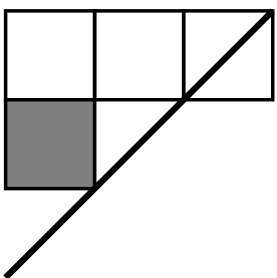
Figure 13: The Dyck ribbon

So the only partition $\lambda-r_{\rm d}$ appearing in the sum on the right hand side of (76) is $(3)$. Thus, from (76), the action of $T_{2}(u_{1}+1)$ on KL_(3,1) is

1= 21+y1​ 1+321,subscript𝑇2subscript𝑢11fragments 1missing-subexpressionmissing-subexpressionfragments 2missing-subexpressionmissing-subexpression1missing-subexpressionmissing-subexpressionsubscript𝑦1fragments 1missing-subexpressionmissing-subexpression321\displaystyle T_{2}(u_{1}+1)\hskip 5.69054pt\begin{tabular}[]{|S|*{\value{sqcolumns}}{Z|}}\hline\cr 1.58334pt]{0.0pt}{6.83331pt}$\scriptstyle 3$\@add@centering&$\scriptstyle 2$\@add@centering&$\scriptstyle 1$\@add@centering\\ \hline\cr 1.58334pt]{0.0pt}{6.83331pt}$\scriptstyle 1$\@add@centering\cr\cline{1-1}\cr\end{tabular}=\begin{tabular}[]{|S|*{\value{sqcolumns}}{Z|}}\hline\cr 1.58334pt]{0.0pt}{6.83331pt}$\scriptstyle 3$\@add@centering&$\scriptstyle 2$\@add@centering&$\scriptstyle 1$\@add@centering\\ \hline\cr 1.58334pt]{0.0pt}{6.83331pt}$\scriptstyle 2$\@add@centering\cr\cline{1-1}\cr 1.58334pt]{0.0pt}{6.83331pt}$\scriptstyle 1$\@add@centering\cr\cline{1-1}\cr\end{tabular}+\hskip 5.69054pty_{1}\begin{tabular}[]{|S|*{\value{sqcolumns}}{Z|}}\hline\cr 1.58334pt]{0.0pt}{6.83331pt}$\scriptstyle 3$\@add@centering&$\scriptstyle 2$\@add@centering&$\scriptstyle 1$\@add@centering\\ \hline\cr 1.58334pt]{0.0pt}{6.83331pt}$\scriptstyle 1$\@add@centering\cr\cline{1-1}\cr\end{tabular}+\hskip 5.69054pt\begin{tabular}[]{|S|*{\value{sqcolumns}}{Z|}}\hline\cr 1.58334pt]{0.0pt}{6.83331pt}$\scriptstyle 3$\@add@centering&$\scriptstyle 2$\@add@centering&$\scriptstyle 1$\@add@centering\\ \hline\cr\end{tabular},

3 2 1 3 2 1 3 2 1 3 2 1 3 2 1 3 2 1

in agreement with the result from the expansion (74), using the (75).

From (74) we can also deduce recursions between the coefficients $c_{\lambda}$. For example, it is clear that $c_{3,2,1}=c_{2,1}$, and that $c_{3,2}=y_{1}c{2,1}$. In fact, all coefficients corresponding to two-row diagrams have a factor $y_{1}$, while others do not contain such a factor. Careful considerations lead to the recursion as explained in the main text.

References

- Kazhdan and Lusztig [1979] D. Kazhdan, G. Lusztig, Representations of Coxeter groups and Hecke algebras, Inv. Math. (1979) 165–184.
- Young [1952] A. Young, Quantitative substitutional analysis I-IX, Proc. London Math. Soc. (1901–1952).
- Hoefsmit [1974] P. Hoefsmit, Representations of Hecke algebras of finite groups with BN-pairs of classical type, PhD Thesis, University of British Columbia (1974).
- Deodhar [1987] V. Deodhar, One some geometric aspects of Bruhat orderings. II. The parabolic analogue of Kazhdan-Lusztig polynomials, J. Algebra 111 (1987) 483–506.
- Cherednik [1993] I. Cherednik, Double affine Hecke algebras, Knizhnik-Zamolodchikov equations, and Macdonalds operators, Int. Math. Res. Not. 9 (1993) 171–180.
- D. Bernard and Pasquier [1993] D. H. D. Bernard, M. Gaudin, V. Pasquier, Yang-Baxter equation in spin chains with long range interactions, J. Phys. A 26 (1993) 5219–5236.
- Macdonald [1996] I. Macdonald, Affine Hecke algebras and orthogonal polynomials, Astérisque 237 (1996) 189–207.
- Pasquier [2006] V. Pasquier, Quantum incompressibility and Razumov stroganov type conjectures, Ann. Henri Poincaré 7 (2006) 397–421, arXiv:cond-mat/0506075.
- Bernevig and Haldane [2008] B. Bernevig, F. Haldane, Model fractional quantum Hall states and Jack polynomials, Phys. Rev. Lett. 100 (2008) 246802 (4 pages), arXiv:0707.3637.
- Di Francesco and Zinn-Justin [2005] P. Di Francesco, P. Zinn-Justin, The quantum Knizhnik Zamolodchikov equation, generalized Razumov Stroganov sum rules and extended Joseph polynomials, J. Phys. A: Math. Gen. 38 (2005) L815--L822, arXiv:math-ph/0508059.
- Kasatani and Pasquier [2007] M. Kasatani, V. Pasquier, On polynomials interpolating between the stationary state of a O(n) model and a Q.H.E. ground state, Comm. Math. Phys. 276 (2007) 397--435, arXiv:cond-mat/0608160.
- Kasatani and Takeyama [2007] M. Kasatani, Y. Takeyama, The quantum Knizhnik-Zamolodchikov equation and non-symmetric Macdonald polynomials, Funkcialaj Ekvacioj 50 (2007) 491--509, arXiv:math/0608773.
- Di Francesco and Zinn-Justin [2005] P. Di Francesco, P. Zinn-Justin, Around the Razumov-Stroganov conjecture: proof of a multi-parameter sum rule, Electr. J. Comb. 12 (2005) R6, arXiv:math-ph/0410061.
- Di Francesco and Zinn-Justin [2008] P. Di Francesco, P. Zinn-Justin, Quantum Knizhnik--Zamolodchikov equation, totally symmetric self-complementary plane partitions and alternating sign matrices, Theor. Math. Phys. 154 (2008) 331--348, arXiv:math-ph/0703015.
- Di Francesco and Zinn-Justin [2007] P. Di Francesco, P. Zinn-Justin, Quantum Knizhnik Zamolodchikov equation: reflecting boundary conditions and combinatorics, J. Stat. Mech.: Theory and Exp. 12 (2007) P12009, arXiv:0709.3410.
- Zinn-Justin [2007] P. Zinn-Justin, Loop model with mixed boundary conditions, qKZ equation and alternating sign matrices, Journal of Statistical Mechanics: Theory and Experiment 1 (2007) P01007, arXiv:math-ph/0610067.
- de Gier et al. [2009] J. de Gier, A. Ponsaing, K. Shigechi, The exact finite size ground state of the O(n = 1) loop model with open boundaries, J. Stat. Mech.: Theory and Exp. 4 (2009) P04010, arXiv:0901.2961.
- Cantini [2009] L. Cantini, qKZ equations and ground state of the O(1) loop model with open boundary conditions, ArXiv e-prints (2009), arXiv:0903.5050.
- de Gier et al. [2010] J. de Gier, B. Nienhuis, A. Ponsaing, Exact spin quantum Hall current between boundaries of a lattice strip, Nucl. Phys. B (online) (2010), arXiv:1004.4037.
- Blasiak [2011] J. Blasiak, Quantum Schur-Weyl duality and projected canonical bases (2011), arXiv:1102.1453.
- Bressoud [1999] D. Bressoud, Proofs and confirmations. The story of the alternating sign matrix conjecture, Cambridge University Press, 1999.
- Kirillov and Lascoux [2000] A. Kirillov, A. Lascoux, Factorization of Kazhdan-Lusztig elements for Grassmanians, in: Combinatorial methods in representation theory, volume 28 of Adv. Stud. Pure Math., Kinokuniya, Tokyo, 2000, pp. 143--154.
- de Gier and Pyatov [2007] J. de Gier, P. Pyatov, Factorised solutions of Temperley-Lieb KZ equations on a segment, arXiv preprint (2007), arXiv:0710.5362.
- Lascoux [2001] A. Lascoux, Yang-Baxter Graphs, Jack and Macdonald Polynomials, Annals of Combinatorics 5 (2001) 397--424.
- Knop [1997] F. Knop, Symmetric and non-symmetric quantum Capelli polynomials, Comment. Math. Helv. 72 (1997) 84--100.
- Sahi [1998] S. Sahi, The binomial formula for nonsymmetric Macdonald polynomials, Duke Math. J. 94 (1998) 465--477.
- Jimbo and Miwa [1995] M. Jimbo, T. Miwa, Algebraic analysis of solvable lattice models, AMS, Providence, 1995.
- Shigechi and Zinn-Justin [2010] K. Shigechi, P. Zinn-Justin, Path representation of maximal parabolic Kazhdan-Lusztig polynomials, ArXiv e-prints (2010), arXiv:1001.1080.
- Di Francesco [2008] P. Di Francesco, Totally symmetric self-complementary plane partitions and quantum Knizhnik-Zamolodchikov equation: a conjecture, Theor. Math. Phys. 154 (2008) 331--348, arXiv:math-ph/0703015.
- de Gier et al. [2009] J. de Gier, P. Pyatov, P. Zinn-Justin, Punctured plane partitions and the q-deformed Knizhnik--Zamolodchikov and Hirota equations, J. Combin. Theory Ser. A 116 (2009) 772--794, arXiv:0712.3584.
- Fonseca and Zinn-Justin [2008] T. Fonseca, P. Zinn-Justin, On the doubly refined enumeration of alternating sign matrices and totally symmetric self-complementary plane partitions, Electron. J. Combin. 15 (2008) 35 pp, arXiv:0803.1595.
- Fonseca and Nadeau [2010] T. Fonseca, P. Nadeau, On some polynomials enumerating fully packed loop configurations, ArXiv e-prints (2010), arXiv:1002.4187.
- Mills et al. [1986] W. Mills, D. Robbins, H. Rumsey, Self-complementary totally symmetric plane partitions, J. Combi. Theory Ser. A 42 (1986) 277--292.
- Andrews [1994] G. Andrews, Plane partitions V: the TSSCPP conjecture, J. Combin. Theory Ser. A 66 (1994) 28--39.
- Zeilberger [2007] D. Zeilberger, Proof of a conjecture of Philippe Di Francesco and Paul Zinn-Justin related to the qKZ equation and to Dave Robbins’ two favorite combinatorial objects, Personal Journal of S.B. Ekhad and D. Zeilberger (2007), http://math.rutgers.edu/~zeilberg/mamarim/mamarimPDF/diFrancesco.pdf.
- Lascoux [2003] A. Lascoux, Symmetric functions and combinatorial operators on polynomials, volume 99 of CBMS Regional Conference Series in Mathematics, American Mathematical Society, Providence, 2003.
- Manivel [2001] L. Manivel, Symmetric functions, Schubert polynomials and degeneracy loci, volume 6 of SMF/AMS texts and monographs, American Mathematical Society, 2001.
- Fu and Lascoux [2009] A. M. Fu, A. Lascoux, Non-symmetric Cauchy kernels for the classical groups, J. Comb. Theory Ser. A 116 (2009) 903--917, arXiv:math/0612828.
- Macdonald [1995] I. Macdonald, Symmetric functions and Hall polynomials, second edition, Oxford Science Publications, Oxford University Press, 1995.