Three dimensional cooling and detecting of a nanosphere with a single cavity

Abstract

We propose an experimental scheme to cool and measure the three-dimensional (3D) motion of an optically trapped nanosphere in a cavity. Driven by three lasers on TEM00, TEM01, and TEM10 modes, a single cavity can cool a trapped nanosphere to the quantum ground states in all three dimensions under the resolved-sideband condition. Our scheme can also detect an individual collision between a single molecule and a cooled nanosphere efficiently. Such ability can be used to measure the mass of molecules and the surface temperature of the nanosphere. We also discuss the heating induced by the intensity fluctuation, pointing instability, and the phase noise of lasers, and justify the feasibility of our scheme under current experimental conditions.

I introduction

Cooling microscopic, mesoscopic, and macroscopic objects to their motional ground states has attracted great attention in the past decades. Various atoms, ions and molecules have been cooled and trapped, and some of them have been employed in quantum information processing and atomic clocks. It is of fundamental interests to cool macroscopic objects down to quantum regime for studying quantum effects in macroscopic systems, improving precisions in ultra-sensitive measurements Clerk et al. (2010); Anetsberger et al. (2010); Verlot et al. (2010), and realizing quantum information processing with new ideas Mancini et al. (2003); Hammerer et al. (2009); Zhang-qi Yin and Y.-J. Han (2009). Cooling mechanical oscillators near the ground state can be accomplished by placing the high frequency oscillator in cryogenic environment LaHaye et al. (2004); O’Connell and et al. (2010), or optomechanical cavity cooling methods Naik et al. (2006); Gigan et al. (2006); Schliesser et al. (2008); Marquardt et al. (2007); Wilson-Rae et al. (2007), or combining them together Schliesser et al. (2009); Gröblacher et al. (2009); Park and Wang (2009); Rocheleau et al. (2010).

Recent report has shown the possibility to cool a mesoscopic microwave-frequency mechanical oscillator down to the motional ground state by standard cryogenic methods O’Connell and et al. (2010). However, the mechanical Q factor (around 260) in this system O’Connell and et al. (2010) is too small for many applications. Similar to optical trapping and cooling of atoms Vuletić and Chu (2000); Vuletić et al. (2001); Leibrandt et al. (2009) and molecules Schulze et al. (2010); Lev et al. (2008), a nanosphere can be optically trapped and cooled in a cavity Ashkin and Dziedzic (1976); Chang and et al. (2010); Romero-Isart et al. (2010); Romero-Isart et al. (2010). An optically trapped nanosphere in vacuum is well isolated from the thermal environment and can have a mechanical Q factor larger than $10^{10}$. This approach has the potential to cool a mechanical system to the vibrational ground state even at room temperature, based on which nonclassical states(e.g. squeezed states) could be generated. A cooled nanosphere can also be used to test gravity induced decoherence effects Penrose (1996) and search for non-Newtonian gravity forces Geraci et al. (2010).

We noticed that the first part of the proposal Chang and et al. (2010); Romero-Isart et al. (2010), which is trapping micro(nano)-sphere by optical tweezer with high frequency, has been realized experimentally Li et al. (2010), in which a glass microsphere was optically trapped in air and vacuum, and its Brownian motion was measured with ultrahigh precision. A more exciting work would be to cool a nanosphere to the quantum ground state using sideband cooling with the help of cavities Chang and et al. (2010); Romero-Isart et al. (2010), and observe the individual collisions between the sphere and single molecules Epstein (1924).A nanosphere will scatter the cooling laser to all three dimensions and cause 3D heating. The heating effects of laser noises are also 3D. As will be discussed later, such heating can cause exponential growth of the kinetic energy of a nanosphere. If only one-dimensional motion is cooled efficiently, the others will be heated up continuously and the nanosphere will be kicked out of the trap. In order to achieve ground state cooling of an optically trapped nanosphere, we must use a 3D cooling scheme. We can straightforwardly add two more cavities for cooling the other two dimensions, but the system will become too complex to be realized. We may combine the 1D cavity cooling with 2D feedback cooling to stabilized the system. But the system will also become complex and can only do ground state cooling in 1D.

In this work, we propose to cool and measure the 3D motion of a nanosphere by TEM00, TEM01, and TEM10 modes of a single cavity. We show that each one of these three modes can be coupled to the motion of a trapped nanosphere in each dimension respectively. Thus they can be used to cool and detect the 3D motion of a nanosphere. The scheme can be used for detecting the individual collisions between molecules and the nanosphere. The mass of the molecules, and the surface temperature of the nanosphere may also be measured at the same time. We noticed trapping single atoms in a high-finesse cavity driven by three lasers at TEM00, TEM01, and TEM10 modes simultaneously has been realized in an experiment Puppe and et al. (2007). One can also use a phase plate to generate a TEM01 (or TEM10) beam from a TEM00 beam Meyrath et al. (2005), and use it to pump the corresponding mode of a cavity. Our scheme should also helpful for cavity cooling of atoms (ions) and molecules.

The paper is organized as follows. In Sec. II , we introduce the scheme of nanosphere 3D cooling via a cavity. In Sec. III, we propose the scheme of detecting the collisions between molecules and the sphere, and discuss the experimental possibility. In Sec. IV, we give a short summary of the paper.

II 3D cooling model

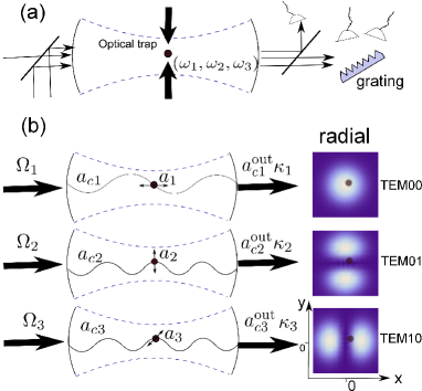
Figure 1: (color online) (a) Cooling and detecting scheme. A nanosphere is trapped by a dual-beam optical tweezer inside of a cavity. The cavity is driven by three lasers in TEM00, TEM01 and TEM10 modes. The TEM01 mode laser has different polarization, and is separated from the other two lasers by a polarizing beam splitter for detection. The TEM00 and TEM01 lasers have different frequencies, and are separated by a grating for detection. (b) Three cooling modes TEM00, TEM01, and TEM10, and their radial distribution. The black dot represents the position of a trapped nanosphere.

As shown in Fig. 1a, we consider an optically trapped nanosphere with mass $m$ confined in a cavity by means of an optical tweezer Li et al. (2010). Since the mechanical Q of the system could be extremely high, e.g., $>10^{10}$ Chang and et al. (2010); Romero-Isart et al. (2010), we may consider an ideal system in the first part of our treatment, but leave the effect from the environment, such as the collisions between molecule and nanosphere, to later discussion. The frequencies of the optical trap along the $z$, $x$, and $y$ axes are $(\omega_{1}$, $\omega_{2}$, and $\omega_{3})$. Contrary to the conventional method of using a cooling laser with TEM00 mode to cool the motion along $z$ direction, we add two non-Gaussian beams with TEM01 and TEM10 modes to drive the cavity in order to cool the motion along the $x$ and $y$ directions, respectively. The resonant frequencies of the cavity modes $a_{c1}$, $a_{c2}$, and $a_{c3}$ are $\omega_{c1}$, $\omega_{c2}$, and $\omega_{c3}$, respectively. The detunings between the lasers and the cavity modes are $\Delta_{cj}=\omega_{c}^{j}-\omega_{L}^{j}$ $(j=1,2,3)$. We suppose that the TEM01 and TEM10 lasers have the same frequency, but with orthogonal polarization. The TEM00 and TEM01 lasers have the same polarization, but different frequencies. In practical, the frequency differences between TEM00 and TEM01 (TEM10) could be very large, and the TEM01 and TEM10 modes are orthogonal in polarizations. Therefore the interference between the three cavity modes can be neglected.

Supposing the radius of the nanosphere to be much smaller than the wavelength of the cavity mode, we may calculate the sphere-induced cavity frequency shift $\delta\omega$ by perturbation theory,

$$\frac{\delta\omega}{\omega_{0}}=-\frac{1}{2}\frac{\int d^{3}{\bf r}\delta P({\bf r})\dot{\bf E}({\bf r})}{\int d^{3}{\bf r}\epsilon_{0}{\bf E}^{2}({\bf r})},$$ (1)

where $\omega_{0}$ is the resonant frequency of a cavity without the nanosphere, ${\bf E}({\bf r})$ is the cavity mode profile and $\delta P({\bf r})$ is the variation in permittivity induced by the nanosphere. Due to the tiny scale of the nanosphere, we have $P({\bf r}^{\prime})\simeq\alpha_{\mathrm{ind}}E({\bf r})\delta({\bf r}-{\bf r}^{\prime})$, with ${\bf r}$ the center-of-mass position of the nanosphere, $\alpha_{\mathrm{ind}}=3\epsilon_{0}V(\frac{\epsilon-1}{\epsilon+2})$ the polarizability, and $V$ the sphere volume.

The total Hamiltonian of the system in the rotating frame is

$$H= \sum_{j=1}^{3}\big{[}\hbar\omega_{j}a_{j}^{\dagger}a_{j}-\hbar(\Delta_{j}-U_{j})a^{\dagger}_{cj}a_{cj}+\frac{\hbar\Omega_{j}}{2}(a_{cj}+a_{cj}^{\dagger})\big{]},$$ (2)

where $a_{j}$ characterizes the phonon mode along $q_{j}$ direction with $q_{1}=z,q_{2}=x,q_{3}=y$. $\Omega_{j}$ is the driving strength by the lasers and $U_{j}$ characterizes the coupling between the cavity mode $a_{cj}$ and the nanosphere. In the limit that $\epsilon\gg 1$, where $\epsilon$ is the electric permittivity of the nanosphere, we get Chang and et al. (2010)

$$U_{1}= -\frac{3V}{2V_{c1}}\exp(-\frac{2x^{2}+2y^{2}}{w^{2}})\cos^{2}(k_{1}z+\varphi_{1})\omega_{c1},$$

$$U_{2}= -\frac{3V}{2V_{c2}}\frac{x^{2}}{w^{2}}\exp(-\frac{2x^{2}+2y^{2}}{w^{2}})\cos^{2}(k_{2}z+\varphi_{2})\omega_{c2},$$

$$U_{3}= -\frac{3V}{2V_{c3}}\frac{y^{2}}{w^{2}}\exp(-\frac{2x^{2}+2y^{2}}{w^{2}})\cos^{2}(k_{3}z+\varphi_{3})\omega_{c3},$$

with $V_{c1}=(\pi/4)Lw^{2}$ and $V_{c2}=V_{c3}=(\pi/16)Lw^{2}$.

We assume the optical tweezer to be much stronger than the cavity-mode-induced trap, and neglect the effects of cooling lights on trapping. Besides, if we carefully choose the location of the trap, such as $z_{0}=0$, $x_{0}=y_{0}=0.25w$, $\varphi_{1}=\pi/4$, and $\varphi_{2}=\varphi_{3}=0$, the gradients of the three light fields lie approximately along the three axes. The effective Hamiltonian is

$$H_{eff}= \sum_{j=1}^{3}\big{[}\hbar\omega_{j}a_{j}^{\dagger}a_{j}-\hbar\Delta_{j}a^{\dagger}_{cj}a_{cj}+\frac{\hbar\Omega_{j}}{2}(a_{cj}+a_{cj}^{\dagger})$$ (3)

$$+\hbar g_{j}a^{\dagger}_{cj}a_{cj}(a_{j}+a_{j}^{\dagger})\big{]},$$

where $g_{j}=q_{\mathrm{zpf}j}\partial U(x,y,z)/\partial j|_{x=x_{0},y=y_{0},z=z_{0}}$ characterizes the coupling strength between the cavity mode and the oscillation of the nanosphere, and $q_{\mathrm{zpf}j}=\sqrt{\hbar/2m\omega_{j}}$ is zero-point fluctuation for the phonon mode $a_{j}$. In general, $g_{1}$ can be one to two orders larger than $g_{2}$ and $g_{3}$. The effective Hamiltonian (3) is deduced with linearization, which is valid when the vibration amplitude of a trapped nanosphere is much smaller than the wavelength of the laser. The rms vibration amplitude of a particle in a harmonic trap is $\sqrt{k_{B}T/(m\omega^{2})}$ . For a nanosphere with radius of $50$ nm trapped in an optical tweezer with trapping frequency of $0.5$ MHz, the vibration amplitude is $20$ nm at $300$ K, and will be only $1.2$ nm at $1$K, which are very small. Thus the linearization will be valid if the nanosphere is pre-cooled by feedback cooling.

From Eq. (3), the linearized Heisenberg equations of motion for our system are,

$$\dot{a_{cj}}= (i\Delta_{cj}^{\prime}-\kappa_{j}/2)a_{cj}-ig_{j}\alpha_{j}(a_{j}+a_{j}^{\dagger})+\sqrt{\kappa_{j}}a_{cj}^{\mathrm{in}},$$ (4)

$$\dot{a_{j}}= -i\omega_{j}a_{j}-ig_{j}(\alpha_{j}a_{cj}^{\dagger}+\alpha_{j}^{*}a_{cj}),$$

where $\alpha_{j}=i\Omega_{j}/(2i\Delta_{cj}^{\prime}-\kappa_{j})$, $\Delta_{cj}^{\prime}=\Delta_{cj}+2g_{j}^{2}|\alpha_{j}|^{2}/\omega_{cj}$, and $\kappa_{j}$ is the decay rate of the cavity mode $a_{cj}$. $\alpha_{j}$ is the amplitude of cavity mode $a_{cj}$. $\Delta^{\prime}_{cj}$ is the effective detuning between the driving laser and the cavity mode $a_{cj}$. The linearization of the Heisenberg equations is valid only if the state is stable. The stable criteria is Genes et al. (2008)

$$S_{1}^{j}= 4\Delta_{cj}^{\prime}\omega_{m}g_{j}^{2}\alpha_{j}^{2}\kappa_{j}^{2}>0$$ (5)

$$S_{2}^{j}= \omega_{m}\Delta_{cj}{{}^{\prime 2}}-g_{j}^{2}\alpha_{j}^{2}\Delta_{cj}^{\prime}>0,$$

Because of $\Delta_{cj}^{\prime}>0$, the criteria $S_{1}^{j}$ are always valid. The criteria $S_{2}^{j}$ are valid only when $g_{j}\alpha_{j}<\sqrt{\omega_{m}\Delta_{cj}^{\prime}}$. In the following discussion, we suppose that the stable criteria (5) is satisfied.

To realize resolved sideband cooling, we require $\omega_{j}\gg\kappa_{j}$. We suppose $|g_{j}\alpha_{j}|\ll\kappa_{j}$, and find that the final phonon number is Clerk et al. (2010)

$$n_{mj}=-\frac{(\omega_{j}+\Delta^{\prime}_{cj})^{2}+(\kappa_{j}/2)^{2}}{4\omega_{j}\Delta^{\prime}_{cj}}.$$

In the special case of $\Delta_{cj}=-\omega^{\prime}_{j}$, the final phonon number is $n_{mj}=(\kappa_{j}/4\omega_{j})^{2}\ll 1$. The cooling rate is $\Gamma_{j}=g_{j}^{2}|\alpha_{j}|^{2}/[\kappa(1+\frac{\kappa_{j}^{2}}{16\omega_{j}^{2}})]$.

III Detecting scheme and noises of the scheme

The scheme can measure the 3D motion of the nanosphere at the same time. We have a reduced equation under rotating wave approximation, in the case of $\Delta_{cj}^{\prime}=-\omega_{j}$ and $\omega_{j}\gg\kappa_{j},\alpha_{j}g_{j}$, as Vitali et al. (2007); Zhang-qi Yin (2009),

$$\dot{a_{cj}}= -\frac{\kappa_{j}}{2}a_{cj}-ig_{j}\alpha_{j}a_{j}+\sqrt{\kappa_{j}}a_{cj}^{\mathrm{in}},$$ (6)

$$\dot{a_{j}}= -ig_{j}\alpha_{j}a_{cj}.$$

In the limit $\kappa_{j}\gg g\alpha_{j}$, using boundary condition $a_{cj}^{\mathrm{out}}=-a_{cj}^{\mathrm{in}}+\sqrt{\kappa_{j}}a_{cj}$, we get $a_{cj}^{\mathrm{out}}=-i\frac{2g\alpha_{j}}{\sqrt{\kappa_{j}}}a_{j}+a_{cj}^{\mathrm{in}}$, $\dot{a}_{j}=-\frac{2g_{j}^{2}\alpha_{j}^{2}}{\kappa}a_{j}-\frac{2ig_{j}\alpha_{j}}{\sqrt{\kappa}}a_{cj}^{\mathrm{in}}$. Therefore the 3D motion of the nanosphere can be measured by detecting the output fields. In the resolved sideband limit, the output field is nearly vacuum, and will have a signal when there are collisions between the residual molecules in vacuum and the nanosphere. Besides, the shot noise can also be neglected in the scheme as it is very small (estimated to be around $10^{-4}$ Hz in Ref Chang and et al. (2010)).

Because a collision between a molecule and a nanosphere is 3D in nature, our 3D scheme will be essential for efficient detecting of the collisions. Detection of individual collisions between single molecules and the nanosphere would lead to a test of the Maxwell-Boltzmann distribution on single-collision level. Considering the gas pressure $P$ at temperature $T_{\mathrm{env}}$, the radius of the sphere $r$, the molecule mass $m_{m}$, we have the collision number per second $N=(2\pi r^{2})P/\sqrt{\pi m_{m}k_{B}T_{\mathrm{env}}/2}$ Epstein (1924), where $k_{B}$ is the Boltzmann constant. The collision time is estimated to be much less than the nanosphere oscillation time scale. The three phonon modes initially in vacuum will be in a state with mean phonon number $n_{j0}$: $\langle a^{\dagger}_{j}(t_{0})a_{j}(t_{0})\rangle=n_{j0}$ after a single collision, where $t_{0}$ is the time when collision happens. For this case, the output field is

$$a_{cj}^{\mathrm{out}}(t)=-i\frac{2g\alpha_{j}}{\sqrt{\kappa_{j}}}\exp[-\frac{2g_{j}^{2}|\alpha_{j}|^{2}}{\kappa_{j}}(t-t_{0})]a_{j}(t_{0})+a_{cj}^{\mathrm{in}},$$

It is easy to find that $\int_{t_{0}}^{\infty}\langle a_{cj}^{\mathrm{out}}(t)a_{cj}^{\mathrm{out}\dagger}(t)\rangle dt=n_{j0}$. This implies that the output-pulse photon number is equal to the increase of the phonon number after the collision. From above discussion, we get the phonon decay time $\tau_{j}=\kappa_{j}/(4g^{2}_{j}|\alpha_{j}|^{2})$, which is also the pulse duration of the output light of mode $a_{cj}$. The phonon number can be measured by detecting the output light pulse. Therefore, $\tau_{j}$ is the measurement time for the phonon mode $a_{j}$ after the collision. Therefore, as long as $\tau_{j}\ll 1/N$, the collision events can be measured individually.

Moreover, to make sure the success of the output field detection, the phonon number after the collision requires to be added by more than one. For the first case, we suppose the collision is completely elastic. Parts of the molecular movement, which is perpendicular to the surface of the collision point, will change in direction after the collision Epstein (1924). The average increase of the phonon number for $a_{j}$ is $n_{j0}=2m_{m}^{2}\langle v_{j}^{2}\rangle/(\hbar\omega_{j}m)$ with $\langle v^{2}_{j}\rangle$ the the mean velocity square along the axis $q_{j}$. As a result, the requirement for the phonon number change could be rewritten as $2k_{B}T_{\mathrm{env}}>\hbar\omega_{j}(m/m_{m})$. If the collision is completely inelastic, the molecule will attach on the surface of the nanosphere for a while before being kicked out Epstein (1924). The output velocity distribution is completely determined by the temperature of the nanosphere surface. The criteria should be either $k_{B}T_{\mathrm{env}}>2\hbar\omega_{j}(m/m_{m})$, or $k_{B}T_{\mathrm{sur}}>2\hbar\omega_{j}(m/m_{m})$, where $T_{\mathrm{sur}}$ is the temperature of the surface of the nanosphere. To distinguish elastic and inelastic collision, we can cool the temperature to the limit that $k_{B}T_{\mathrm{env}}\ll\hbar\omega_{j}(m/m_{m})$, and makes the condition $k_{B}T_{\mathrm{sur}}>2\hbar\omega_{j}(m/m_{m})$ fulfills by adding a long wavelength laser to heat the sphere. If the collisions are all elastic, there is no signal on the photon detectors. If there are parts of the collisions are inelastic, there are output pulses of lights. Besides, the distribution of the photon numbers is determined by the surface temperature of the sphere. In other words, we can measure the surface temperature of the nanosphere by detecting the output light pulses.

Besides, if there are more than one type of molecules involved, we can also distinguish them by the measurement. We suppose that the energy increasing of the phonon mode $a_{j}$ after collision fulfills the Maxwell-Boltzmann distribution and the collisions are elastic. The mean phonon increasing for mode $a_{j}$ is $n_{j0}=1/(e^{\hbar\omega_{j}/k_{B}T_{j}}-1)=2k_{B}T_{\mathrm{env}}m_{a}/(\hbar\omega_{j}m)$, where $T_{j}$ is the effective temperature of mode $a_{j}$ after single collisions. The phonon adding distribution after single collisions for mode $a_{j}$ is $f(n_{j})dn=\frac{2}{\sqrt{\pi}}(\frac{\hbar\omega_{j}}{k_{B}T})^{3/2}\exp(-n\frac{\hbar\omega_{j}}{k_{B}T})dn$ Laurendeau (2005). However, the mean phonon adding cannot be measured from a single light pulse. As the photon detector can only measure the photon pulses number in integer. The measured number distribution of the mode $a_{j}$ should be Bose-Einstein distribution, which is $f(n_{j})=n_{j0}^{n_{j}}/(1+n_{j0})^{n_{j}+1}$ Scully and Zubairy (1997). We suppose the mass $m_{a}$ and $m_{b}$ corresponding to the molecules $a$ and $b$, respectively, and the same mean kinetic energies for both types of the molecules. The average increase of the phonon number for the phonon modes $a_{j}$ is different for different collision. As shown in Fig. 2a, there are two curves in the phonons distribution of mode $a_{3}$, which represent the two different molecules. Fig. 2b shows The measured phonon distribution for different molecules. We can distinguish the different molecules from data fitting.

Specifically, we consider the example below. We consider a sphere with radius $r=50$ nm and mass $m=1.03\times 10^{-18}$ kg ($\rho=1.96\mathrm{g/cm}^{3}$). The optical tweezer is consturcted with a laser with power $P_{t}=25$mW at wavelength $\lambda=1500$nm, and a lense of numerical aperture $N=0.9$. The trap frequency is $(\omega_{1},\omega_{2},\omega_{3})/2\pi\simeq(0.5,0.5,0.2)$ MHz Romero-Isart et al. (2010). We consider the cavity with length $L=5$ mm, mode waist $\omega=10\mu$m and wavelength $1.5\mu$m. In the case of $\epsilon\gg 1$, we have $g_{z}=52.2$ Hz, $g_{x}=g_{y}=2.2$ Hz, and the zero point fluctuation $(z,x,y)_{\mathrm{zpf}}=\sqrt{\hbar/(2mw_{j})}=(4.0,4.0,6.4)\times 10^{-12}$ m. In order to have the final phonon number $n_{1,2,3}<1$, the finesse of the cavity should be around $10^{5}$. For $m_{m}=6.63\times 10^{-26}$kg and the gas pressure $10^{-10}$Torr, the collision events per second are about $10$. If we suppose the cavity decay rate to be $\kappa=0.5$ MHz, corresponding to finesse $2\times 10^{5}$, with proper driving strength ($|\alpha_{1}|^{2}\sim 5\times 10^{4}$, $|\alpha_{2}|^{2}\simeq 2.5\times 10^{7}$, $|\alpha_{3}|^{2}\sim 10^{7}$), the cooling rate for all three modes would be $10^{2}$Hz and the mean addition of the phonon number for $a_{j}$ after each collision is around $4$. Therefore individual measurements for the collision events can be distinguished for the three phonon modes. The cooling laser power for cavity mode $a_{c1}$ is in the order of $10^{-8}$W, The laser powers for cavity modes $a_{c2}$ and $a_{c3}$ are in the order of $10^{-5}$W.

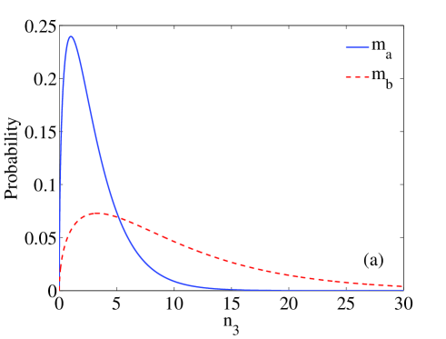
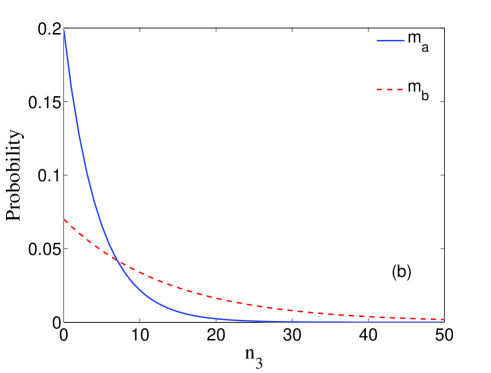
Figure 2: (color online) (a) Distribution of the mean phonon increase, (b) measured phonon number increase distribution of a mechanical mode $a_{3}$ after a elastic collision between the nanosphere and a molecule with mass $m_{a}=6.63\times 10^{-26}$ kg or $m_{b}=2.18\times 10^{-25}$ kg. The temperature of the gas is $300$K.

So far we haven’t considered the systematic noise effects in our treatment. In real experiments, however, the noise from lasers may be fatal to the success of an experiment. We first consider the heating effects from the optical trap Savard et al. (1997). If we want to realize motional ground state cooling of the nanosphere, the heating rate should be much smaller than the laser cooling rate. Strictly speaking, the heating comes from the laser intensity fluctuation and the laser-beam-pointing noise. For the former, we define the fluctuations of the laser $\epsilon(t)=(I(t)-I_{0})/I_{0}$, with $I_{0}$ the average intensity and $I(t)$ the laser intensity at time $t$. By using first-order time-dependent perturbation theory, we get $\langle\dot{E}\rangle=\frac{\pi}{2}\omega_{j}^{2}S_{\epsilon}(2\omega_{j})\langle E\rangle$ Savard et al. (1997). The heating constant is $\Gamma_{\epsilon}=\frac{\pi}{2}\omega_{j}^{2}S_{\epsilon}(2\omega_{j})$, where $S_{\epsilon}(\omega)=\frac{2}{\pi}\int^{\infty}_{0}d\tau\cos(\omega\tau)\langle\epsilon(t)\epsilon(t+\tau)\rangle$ is the one-sided power spectrum of the fractional intensity noise, which could be on the order of $10^{-14}\mathrm{Hz}^{-1}$. For the trap frequency of MHz, $\Gamma_{\epsilon}$ approaches the order of $10^{-1}$Hz. The laser-beam-pointing noise is originated from the fluctuation relevant to the location of the trap center, which is independent of the phonon energy. Similarly, we may get $\langle\dot{E}\rangle=\frac{\pi}{2}m\omega_{j}^{4}S_{j}(\omega_{j}),$ where $j=x,y,z$, and $S_{j}(\omega)$ is the noise spectrum of location fluctuations. We define the heating rate as $\Gamma_{j}=\frac{\pi}{2}m\omega_{j}^{4}S_{j}(\omega_{j})/(\hbar\omega_{j})$, which represents phonon number increase per second. If we set $\Gamma_{j}$ to be on the order of $10^{-1}$Hz, we should make sure that $S_{j}(\omega_{j})$ is around $10^{-35}\mathrm{m}^{2}/$Hz for $\omega_{j}\sim 1$MHz. Experimentally $S_{j}(\omega)$ has been controlled less than $10^{-34}\mathrm{m}^{2}/$ Hz for $\omega\sim 2\pi$ kHz Corbitt and et al. (2007). With the increase of the optical trap frequency to large detuning from the system’s resonant frequency, $S_{j}(\omega_{j})$ is dropping down quickly. Therefore, we believe that the laser-beam-pointing noise could be well controlled and the heating rate $\Gamma_{j}$ would be less than $0.1$ Hz.

The phase noise induced by the cooling laser also need to be seriously considered Diósi (2008); Rabl et al. (2009); Zhang-qi Yin (2009). Because the cooling laser is of finite linewidth, the laser field can be wrote down as $\varepsilon(t)=\varepsilon e^{i\phi(t)}$. We assume the phase noise $\phi(t)$ to be Gaussian and with zero mean value. For the Lorentzian noise spectrum with $S_{\dot{\phi}}(\omega)=2\Gamma_{L}\gamma_{c}/(\gamma_{c}^{2}+\omega^{2})$, and correlation function $\{\dot{\phi(s)}\dot{\phi(s^{\prime})}\}=\Gamma_{L}\gamma_{c}\exp(-\gamma_{c}|s-s^{\prime}|)$, where $\Gamma_{L}$ is the linewidth of the laser and $\gamma_{c}^{-1}$ is the correlation time of the laser phase noise, the phonon number limited by this noise is $n_{ph}>n_{c}\frac{\Gamma_{L}}{\kappa}\frac{\gamma_{c}^{2}}{\gamma_{c}^{2}+\omega_{j}^{2}}$ Rabl et al. (2009). If we choose $\Gamma_{L}=1$ kHz, $\gamma_{c}=3$ kHz, $\omega_{j}=10^{6}$ Hz, and $n_{c}=10^{7}$, we have $n_{ph}\ll 1$. In this sense, like above discussed noise effects, the phase noise effect can also be neglected.

IV conclusion

In conclusion, we have proposed a scheme to cool and measure the 3D motion of an optically trapped nanosphere confined in a single cavity, driven by three lasers. With properly locating the optical trap and the laser detunings, we have shown by calculation that the 3D motion of the nanosphere could be cooled and detected simultaneously, and down to ground states if the sideband resolved condition is fulfilled. We have justified the experimental feasibility of our scheme under currently available technology. We argue that our scheme would be useful for not only checking the Maxwell-Boltzmann distribution at single-collision level, but also measuring the temperature of the surface of the nanosphere and the mass of the molecule.

The work is supported by NNSFC under Grant No. 10974225, by CAS and by NFRPC. TL would like to thank M. G. Raizen for helpful discussions and the suggestion of using a cooled bead to detect single molecules.

Note added: After submitting the paper, we have found a related experimental paper Zhang et al. (2010), which eliminates degenerate trajectory of single atom strongly coupled to the tilted cavity TEM10 mode.

References

- Clerk et al. (2010) A. Clerk, S. Girvin, F. Marquardt, and R. Schoelkopf, Rev. Mod. Phys. 82, 1155 (2010).
- Anetsberger et al. (2010) G. Anetsberger, E. Gavartin, O. Arcizet, Q. P. Unterreithmeier, E. M. Weig, M. L. Gorodetsky, J. P. Kotthaus, and T. J. Kippenberg, ArXiv e-prints (2010), eprint 1003.3752.
- Verlot et al. (2010) P. Verlot, A. Tavernarakis, T. Briant, P.-F. Cohadon, and A. Heidmann, Phys. Rev. Lett. 104, 133602 (2010).
- Mancini et al. (2003) S. Mancini, D. Vitali, and P. Tombesi, Phys. Rev. Lett. 90, 137901 (2003).
- Hammerer et al. (2009) K. Hammerer, M. Aspelmeyer, E. S. Polzik, and P. Zoller, Phys. Rev. Lett. 102, 020501 (2009).
- Zhang-qi Yin and Y.-J. Han (2009) Zhang-qi Yin and Y.-J. Han, Phys. Rev. A 79, 024301 (2009).
- LaHaye et al. (2004) M. D. LaHaye, O. Buu, B. Camarota, and K. C. Schwab, Science 304, 74 (2004).
- O’Connell and et al. (2010) A. O’Connell and et al., Nature 464, 697 (2010).
- Naik et al. (2006) A. Naik, O. Buu, M. D. Lahaye, A. D. Armour, A. A. Clerk, M. P. Blencowe, and K. C. Schwab, Nature (London) 443, 193 (2006).
- Gigan et al. (2006) S. Gigan, H. R. Böhm, M. Paternostro, F. Blaser, G. Langer, J. B. Hertzberg, K. C. Schwab, D. Bäuerle, M. Aspelmeyer, and A. Zeilinger, Nature (London) 444, 67 (2006).
- Schliesser et al. (2008) A. Schliesser, R. Rivière, G. Anetsberger, O. Arcizet, and T. J. Kippenberg, Nature Phys. 4, 415 (2008).
- Marquardt et al. (2007) F. Marquardt, J. P. Chen, A. A. Clerk, and S. M. Girvin, Phys. Rev. Lett. 99, 093902 (2007).
- Wilson-Rae et al. (2007) I. Wilson-Rae, N. Nooshi, W. Zwerger, and T. J. Kippenberg, Phys. Rev. Lett. 99, 093901 (2007).
- Schliesser et al. (2009) A. Schliesser, O. Arcizet, R. Rivière, G. Anetsberger, and T. J. Kippenberg, Nature Phys. 5, 509 (2009).
- Gröblacher et al. (2009) S. Gröblacher, J. B. Hertzberg, M. R. Vanner, G. D. Cole, S. Gigan, K. C. Schwab, and M. Aspelmeyer, Nature Phys. 5, 485 (2009).
- Park and Wang (2009) Y. Park and H. Wang, Nature Phys. 5, 489 (2009).
- Rocheleau et al. (2010) T. Rocheleau, T. Ndukum, C. Macklin, J. B. Hertzberg, A. A. Clerk, and K. C. Schwab, Nature (London) 463, 72 (2010).
- Vuletić and Chu (2000) V. Vuletić and S. Chu, Phys. Rev. Lett. 84, 3787 (2000).
- Vuletić et al. (2001) V. Vuletić, H. W. Chan, and A. T. Black, Phys. Rev. A 64, 033405 (2001).
- Leibrandt et al. (2009) D. R. Leibrandt, J. Labaziewicz, V. Vuletić, and I. L. Chuang, Phys. Rev. Lett. 103, 103001 (2009).
- Schulze et al. (2010) R. J. Schulze, C. Genes, and H. Ritsch, Phys. Rev. A 81, 063820 (2010).
- Lev et al. (2008) B. L. Lev, A. Vukics, E. R. Hudson, B. C. Sawyer, P. Domokos, H. Ritsch, and J. Ye, Phys. Rev. A 77, 023402 (2008).
- Ashkin and Dziedzic (1976) A. Ashkin and J. M. Dziedzic, Appl. Phys. Lett. 28, 333 (1976).
- Chang and et al. (2010) D. E. Chang and et al., PNAS 107, 1005 (2010).
- Romero-Isart et al. (2010) O. Romero-Isart, M. Juan, R. Quidant, and J. Cirac, New J. Phys. 12, 033015 (2010).
- Romero-Isart et al. (2010) O. Romero-Isart, A. C. Pflanzer, M. L. Juan, R. Quidant, N. Kiesel, M. Aspelmeyer, and J. I. Cirac, ArXiv e-prints (2010), eprint 1010.3109.
- Penrose (1996) R. Penrose, Gen. Rel. Grav. 28, 1572 (1996).
- Geraci et al. (2010) A. A. Geraci, S. B. Papp, and J. Kitching, Phys. Rev. Lett. 105, 101101 (2010).
- Li et al. (2010) T. Li, S. Kheifets, D. Medellin, and M. G. Raizen, Science 328, 1673 (2010).
- Epstein (1924) P. S. Epstein, Phys. Rev. 23, 710 (1924).
- Puppe and et al. (2007) T. Puppe and et al., Phys. Rev. Lett. 99, 013002 (2007).
- Meyrath et al. (2005) T. Meyrath, F. Schreck, J. Hanssen, C. Chuu, and M. Raizen, Opt. Express 13, 2843 (2005).
- Genes et al. (2008) C. Genes, D. Vitali, P. Tombesi, S. Gigan, and M. Aspelmeyer, Phys. Rev. A 77, 033804 (2008).
- Vitali et al. (2007) D. Vitali, S. Gigan, A. Ferreira, H. R. Böhm, P. Tombesi, A. Guerreiro, V. Vedral, A. Zeilinger, and M. Aspelmeyer, Phys. Rev. Lett. 98, 030405 (2007).
- Zhang-qi Yin (2009) Zhang-qi Yin, Phys. Rev. A 80, 033821 (2009).
- Laurendeau (2005) N. M. Laurendeau, Statistical Thermodynamics: Fundamentals and Applications (Cambridge Unversity Press, Cambridge, 2005).
- Scully and Zubairy (1997) M. O. Scully and M. S. Zubairy, Quantum Optics (Cambridge Unversity Press, Cambridge, 1997).
- Savard et al. (1997) T. A. Savard, K. M. O’Hara, and J. E. Thomas, Phys. Rev. A 56, R1095 (1997).
- Corbitt and et al. (2007) T. Corbitt and et al., Phys. Rev. Lett. 99, 160801 (2007).
- Diósi (2008) L. Diósi, Phys. Rev. A 78, 021801 (2008).
- Rabl et al. (2009) P. Rabl, C. Genes, K. Hammerer, and M. Aspelmeyer, Phys. Rev. A 80, 063819 (2009).
- Zhang et al. (2010) P. Zhang, Y. Guo, Z. Li, Y. Zhang, J. Du, G. Li, J. Wang, and T. Zhang, ArXiv e-prints (2010), eprint 1012.2156.