Adhesive penetration in Beech wood

Abstract

We propose an analytical model to predict the adhesives penetration into hard wood. Penetration of hard wood is dominated by the vessel network which prohibits porous medium approximations. Our model considers two scales: a one dimensional capillary fluid transport of a hardening adhesive through a single, straight vessel with diffusion of solvent through its walls and a mesoscopic scale based on topological characteristics of the vessel network, where results from the single vessel scale are mapped onto a periodic network. Given an initial amount of adhesive and applied bonding pressure, we calculate the portion of the filled structure. The model is applied to beech wood samples joined with three different types of adhesive (PUR, UF, PVAC) under various growth ring angles. We evaluate adhesive properties and bond line morphologies described in part I of this work. The model contains one free parameter that can be adjusted in order to fit the experimental data.

1 Introduction

The most important principle in timber engineering to produce structural wood components of constant quality, consists of cutting wood into smaller pieces, selecting the best ones, and joining them again by adhesive bondings. What is known as a rather simple processing step becomes quite complicated, once we look in detail at the penetration of the hardening adhesive into the porous wood skeleton. Unfortunately the details of the adhesive penetration can influence bond performance in multiple ways and the quality of the adhesive bonds determine the overall performance of structural parts marra-92 ; Custodio-etal-2009 . What complicates studies of adhesive penetration is the interplay between pore space geometry and fluid transport, cell wall material and adhesive rheology and of course process parameters like amount of adhesive, growth ring orientation, and surface roughness, just to name a few kamke-lee-2007 . While for soft wood predictions are rather simple, the micro-structure of hard woods complicates the problem significantly, since adhesives can penetrate through the big vessel network deep into the wood structure siau-84 . In a previous work we explored the topological characteristics of the vessel network in beech (Fagus sylvatica L.) philipp-09 and showed in part I of this work how the problem is dominated by flow through the vessel network.

Adhesive penetration into hard wood was studied before wang-yan-2005 ; kamke-lee-2007 ; sernek-resnik-kamke-99 ; niemz-etal-2004 ; collett-72 , although only experimentally or in descriptive form. For soft wood, the penetration depth can be expressed by a simple trigonometric function, describing the filling of cut tracheids suchsland-58 . For hard wood however a model that characterizes the wood anatomy in order to predict the penetration depth and the amount of adhesive inside the structure is unknown. We construct an analitycal model based on the network properties and predict the adhesive penetration and the saturation of the vessel pore space. Our model has two-scales: the first scale describing the transport of a hardening adhesive through a single vessel in time due to an applied pressure and capillarity effects, and also with the possibility of constant diffusion of solvent through the vessel wall, what turns out to be important for some adhesives like PVAC or UF. When the viscosity increases by hardening and/or loss of solvent, the adhesive front slows down and finally stops. On the second, or network scale, the result for single vessels is embedded into a network model with identical topological properties like pore size distribution and connectivity that are characteristic for the vessel network of the respective wood. The model is compared with experiments where specimens are bonded with parallel longitudinal axes under varying growth ring angles using three different adhesive systems: PRF, UF, and PVAC. First we describe the rheological model of the adhesives, before we calculate the penetration into a single vessel with diffusion into the half space. Subsequently we discuss the network construction and the consideration of process parameters. With all model components at our hands, we finally compare the model with the experiments and discuss the results.

2 Model Description

Adhesive penetration is the result of an interplay of adhesive hardening, capillary penetration, and technological processing. In order to set up a model for adhesive penetration of hard wood, we have to combine several models in a hierarchical way. First we address bulk viscosity evolution of adhesives due to generic hardening mechanisms. On the fundamental level, we model the penetration of a fluid into one single, straight or wavy pipe. This model is enriched by diffusive transport of solvent through its wall. On the next hierarchic level, we project the fundamental model onto a network structure of perfectly aligned hard wood that represents the vessel network. Finally, we rotate the result of the vessel network penetration to consider the general situation, where the adhesive surface is not necessarily aligned to the material orientation. We show how material parameters like porosity, hardening time or applied amount of adhesive will limit penetration.

2.1 Modeling the hardening process

The hardening process of various adhesives can be described by the temporal evolution of the viscosity $\eta$. Depending on the hardening type, different viscosity models need to be applied. For example reactive adhesives do not depend on the solvent concentration, while the viscosity evolution of solvent based adhesives strongly depends on solvent concentration $C$. In part I part1 of this work, we showed experimental viscosity measurements for UF, PVAC, and PUR. If solvent concentrations are important, like in the case of PVAC, the viscosity evolution can be expressed by

$$\eta(C,t)=\eta_{g}(C)[1+\gamma(C)\exp(\alpha(C)t)]\exp(\beta[1-C])\quad,$$ (1)

where $\eta_{g}$, $\gamma$, $\alpha$ and $\beta$ are parameters that depend on the adhesive type and the initial solvent concentration. For PVAC adhesive, we find $\gamma$$=$$\alpha$$=$$0$, since the hardening process is mostly due to the loss of moisture and the initial viscosity only depends on the initial concentration. For PUR adhesive, the same expression can be used, however the concentration is kept constant during the process, expressed by $\beta$$=$$0$ and constant $\eta_{g}$, $\gamma$, $\alpha$ that only depend on the initial concentration.

Unfortunately a whole class of adhesives, cannot be described by Eq. 1, since their hardening process is more complex. For example the UF adhesive changes from liquid phase to gel phase during penetration, resulting in penetration arrest. The only active processes after this phase transition are the chemical curing reactions. Therefore the viscosity model should take into account the critical time when the phase transition occurs. Additionally, the concentration of the solvent changes in time due to the diffusion of the solvent into the cell wood structure. We propose the viscosity relation

$$\eta_{\rm UF}(C,t)=d_{1}\frac{\exp\left(b_{2}\left(1-\exp\left(-\frac{a_{1}}{t}\right)\right)\right)}{c_{1}-t}\quad,$$ (2)

where $d_{1}$, $b_{2}$, $a_{1}$ and $c_{1}$ are experimental parameters. Using the data from Ref. part1 we found $d_{1}$$=$$6.985\times 10^{4}$ mPa$\cdot$s² and $a_{1}$$=$$10510$s and variable parameters ($b_{2}$ and $c_{1}$) that depend on the initial solvent concentration. Note that $c_{1}$ describes the time when the penetration process finishes due to the liquid-gel transition. Using these two generic hardening models, we are able to describe the viscosity evolution of numerous adhesives.

2.2 Single vessel penetration

The fundamental scale is given by the capillary transport of a fluid characterized by its viscosity $\eta$, inside a cylindrical pipe of radius $R$ washburn-21 with a penetration rate $dl/dt$ that follows

$$\frac{dl}{dt}=\frac{\mu}{8\eta l}R^{2}\quad,$$ (3)

where $\mu=P_{A}+2\sigma\cos(\theta)/R$ with the applied pressure $P_{A}$, the surface tension $\sigma$ and the contact angle between fluid and pipe wall $\theta$. To obtain the penetrated distance $l(t)$ we integrate

$$l(t)=\frac{R}{2}\sqrt{\mu\int_{0}^{t}\frac{1}{\eta(u)}du}\quad,$$ (4)

leading to a total fluid volume of $V_{p}=\pi R^{2}l(t)$ inside the pipe. For reactive adhesives, whose hardening only depends on time, the integral can be found by combining Eqs. 1 and 4 to

$$l(t)=\frac{R}{2}\sqrt{\mu}\left(\frac{\alpha t-\log(1+\gamma\exp^{\alpha t})}{\alpha\eta_{g}\exp^{\beta(1-C)}}\right)^{\frac{1}{2}}\quad.$$ (5)

This way we obtain the time dependent penetration distance in a straight single vessel, taking into account the applied pressure, the capillarity effects, and the reactive hardening process. Note that for adhesive types, whose viscosity changes when in contact with wood, Eq. 4 can not be integrated so easily, since the viscosity depends also on the concentration that changes with time. Note that changes of the contact angle and furface tension of the adhesives with solvent concentration are not considered in this work.

Since hard wood vessels are not straight, but weave tangentially around rays, the penetration distance needs to be modified. Here we simply describe vessels by the radius $R$, wavelength $\lambda$, and amplitude $n$ (see Fig. 1) of the oscillation in the $z-y$-plane in the parametrized form as,

$$x^{2}+\frac{[y-n\cos(kz)]^{2}}{\sec^{2}[\arctan(nk\sin(kz))]}=R^{2}\quad,$$ (6)

where $k=2\pi/\lambda$. By integrating the vessel length $l_{v}$ along the $z$ direction, we obtain the volume

$$V(l_{v})=\pi R^{2}l_{v}\left[1+\frac{n^{2}k^{2}}{4}\left(1+\frac{\sin(2kl_{v})}{2kl_{v}}\right)\right]\quad.$$ (7)

2.3 Viscosity increase by diffusion

Various adhesives contain solvents, whose concentration $C$ in the mixture changes with time due to their diffusion into the cellular structure through vessel walls. To take this effect into account, we can write the solution of the diffusion equation in cylindrical $z-r$-coordinates as

$$C(r,t)=\frac{C_{0}}{2Dt}\exp\left(-\frac{r^{2}}{4Dt}\right)\quad,$$ (8)

with the initial concentration of the solvent $C_{0}$ and its diffusivity across the cell wall $D$. The average diffusivity of the respective wood proved to be a good value. The mean value for the solvent concentration inside the vessel follows as

$$\overline{C}=\int_{0}^{R}C(r,t)rdr=C_{0}\left[1-\exp\left(-\frac{R^{2}}{4Dt}\right)\right]\quad.$$ (9)

To obtain the complete equation for the evolution of the viscosity, we go back to Eq. 1 and insert the concentration evolution $\overline{C}$ into the respective concentration dependent parameters. Note that we do not consider the diffusion of low molecular parts of the adhesive. We also neglect the effect of swelling of the wood skeleton due to moisture changes, since the size of vessels is rather big compared to tracheids.

2.4 Penetration into the network

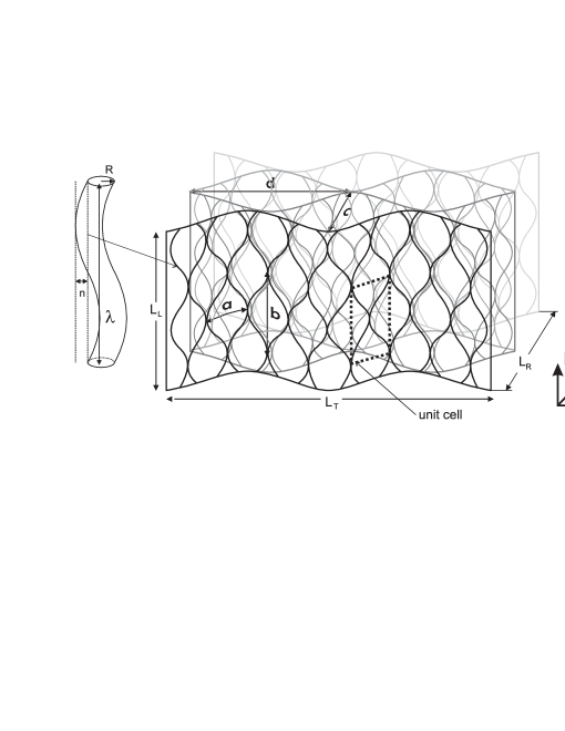
Figure 1: Vessel geometry and dimensions, vessel network, and unit cell. Shown are also the longitudinal ($L$), tangential ($T$), and radial ($R$) directions.

The adhesive penetration is dominated by the flow inside the vessel network, hence its topology determines the adhesive distribution. The network is formed by bundles of vessels that divide and weave around rays of various sizes. Inside the bundle, vessels interconnect by contact zones when touching each other and can also interchange positions philipp-09 ; bosshard-73 . Disorder in the network can only be considered through a numerical approach. In order to be able to derive an analytical model, we need to neglect disorder and use average topological network parameters. We build up a regular network using the average topological parameters $a$ and $b$ for connectivity in tangential directions and $c$, $d$ for the connectivity in radial direction. Fig. 1 shows the vessel network in three dimensions with the geometrical parameters $a$, $b$, $c$ and $d$. Note that $a$ and $b$ can be obtained from the size distribution of big and middle sized rays that are mainly responsible for the splitting and joining of the bundles of vessels. The parameters $c$ and $d$ however are more difficult to obtain. Basically the probability for radial network interconnections depends on the vessel density. We can therefore find a relation between the vessel density and the parameter $c$. $d$ however will remain a free parameter for transport in radial direction. By separating the two geometric parameters $a$, $b$ and $c$, $d$, we obtain anisotropic transport in the three principal directions, longitudinal $L$, radial $R$, and tangential $T$ (see Fig. 1). Note that inclined samples with respect to the principal axis can be considered after rotation.

To describe the penetration process of adhesives into wood, we have to define the bond line. The bondline is the whole region, where the adhesive can be found. This includes the pure adhesive between the two adherends and the area, where the adhesive has penetrated into the wood structure. The adherends are two pieces of wood which have been connected by the adhesive. In our case, we will focus on the zone where the adhesive layer and the adherent structure coexist. The procedure to obtain the maximum penetration depth is to calculate the penetration separately in each principal direction (tangential $T$, radial $R$, and longitudinal $L$, shown in Fig. 1) and then applying a rotation matrix to find the total penetration depth of the adhesive when the growth ring angle and the angle between vertical and longitudinal axis of the specimen are not zero.

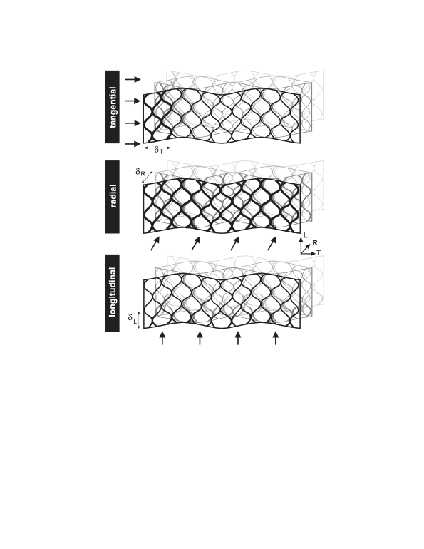
Figure 2: Adhesive penetration into the vessel network with respective depths in tangential ($\delta_{T}$), radial ($\delta_{R}$), and longitudinal ($\delta_{L}$) direction. Thick lines represent filled vessels.

Since we employ a regular network, a unit cell can be used that consists of two single vessels with interconnections in the vertices and the center of the cell (see Fig. 1). Consequently we can use Eq. 7 of the single vessel to obtain the volume of the unit cell

$$V_{u}=2Abg_{T}\quad\text{with}\quad g_{T}=1+\frac{a^{2}\pi^{2}}{16b^{2}}$$ (10)

with the area $A=\pi R^{2}$. Because the unit cell can reproduce all the network, we can use it to simplify the calculation of the penetration depth on each direction and, using geometric properties, we can relate the adhesive volume inside the network, the network parameters and the penetration depth.

2.4.1 Penetration in the tangential direction

To consider the penetration in the tangential direction (see Fig. 2), we need to consider additionally to the tangential waviness with wavelength $b$ and amplitude $a/4$ the radial waviness with amplitude $c/4$ and wavelength $d$. Fig. 2 shows how the vessel network is filled by the adhesive. The path along one radial wave as function of the tangential coordinate $x_{T}$ is given by

$$s_{b}=x_{T}\left[1+\frac{1}{2}\left(g_{R}-1\right)\left(1+\frac{d}{4\pi x_{T}}\sin\left(\frac{4\pi x_{T}}{d}\right)\right)\right]\quad\text{with}\quad g_{R}=1+\frac{c^{2}\pi^{2}}{8d^{2}}~{}~{}.$$ (11)

The number of layers accessible from the bond line is defined by $2L_{R}/c$ with $L_{R}$ the sample width. Summing over all accessible layers gives the total penetrated length as function of $x_{T}$

$$s_{total}=\frac{2L_{R}}{c}s_{b}(x_{T})\quad.$$ (12)

To obtain the total penetrated volume we have to calculate the number of unit cells $N_{uL}$ along $s_{total}$ and in longitudinal sample direction $L_{L}$, this is $N_{uL}$=$\frac{s_{total}}{a}\frac{L_{L}}{b}$, and then multiplied by the unit cell volume, Eq. 10,

$$V_{T}(x_{T})=N_{uL}V_{u}\quad.$$ (13)

Assuming that the penetration of the adhesive is smaller than the total wavelength $d$, $\frac{d\sin(4\pi x/d)}{4\pi x}$$\approx$$1$. Therefore using Eqs. 10 and 12, Eq. 13 can be expressed as

$$V_{T}(x_{T})=x_{T}\frac{4A}{ac}L_{R}L_{L}g_{T}g_{R}\quad.$$ (14)

When the adhesive stops to penetrate, this volume becomes the maximum volumen $V$ inside the structure and the tangential coordinate $x_{T}$ transforms in the maximum penetration depth $\delta_{T}$,

$$\delta_{T}=\frac{Vac}{4AL_{R}L_{L}g_{T}g_{R}}\quad.$$ (15)

2.4.2 Penetration in the radial direction

Following the idea of calculating the adhesive penetration in each principal direction, the next step is to obtain the penetration depth $\delta_{R}$ when the adhesive penetrates only in radial direction. Fig. 2 illustrates the penetration of the adhesive in order to relate the volume with the network parameter and the penetration depth. We analogously count the volume occupied by vessels as function of the radial coordinate $x_{R}$. Again we calculate the total length $s_{total}$ of the radial wave but now as function of $x_{R}$ by $s_{total}$$=$$2x_{R}/cs_{b}(L_{T})$ and obtain the number of unit cells

$$N_{uR}(x_{R})=\frac{2x_{R}}{c}\frac{s_{b}(L_{T})}{a}\frac{L_{L}}{b}\quad.$$ (16)

The total volume occupied is given by multiplying the number of unit cells $N_{uR}$ (Eq. 16) by the volume $V_{u}$ from Eq. 10:

$$V_{T}(x_{R})=V_{u}N_{uR}=x_{R}\frac{4A}{ac}L_{L}s_{b}(L_{T})g_{T}\quad.$$ (17)

As before, we must now compare $V_{T}(x_{R})$ with the volume occupied by the adhesive $V$ with the maximum penetration depth in the radial direction $x_{R}=\delta_{R}$ to obtain

$$V=\delta_{R}\frac{4A}{ac}L_{L}s_{b}(L_{T})g_{T}\quad,\quad\text{and}\quad\delta_{R}=\frac{Vac}{4AL_{L}s_{b}(L_{T})g_{T}}\quad.$$ (18)

Finally, we can insert the penetration path from Eq. 11 and obtain

$$\delta_{R}=\frac{Vac}{4AL_{L}L_{T}\left[1+\frac{1}{2}\left(g_{R}-1\right)\left(1+\frac{d\sin\left(\frac{4\pi L_{T}}{d}\right)}{4\pi L_{T}}\right)\right]g_{T}}\quad.$$ (19)

2.4.3 Penetration in the longitudinal direction

We consider now the penetration only in longitudinal direction. Fig. 2 shows that the adhesive penetration $\delta_{L}$ is basically along the vessels. This value is found again by calculating the number of total unit cells, but now in the plane $L_{T}L_{R}$, namely

$$N_{uL}=\frac{2L_{R}}{c}\frac{s_{b}(Lx)}{a}\quad.$$ (20)

Multiplying $N_{uL}$ with the occupied volume $V(x_{L})$ of the adhesive for each vessel as function of $x_{L}$ (Eq. 7), and taking into account that the penetration $x_{L}$$<<$$b$, $\frac{b\sin(4\pi x_{L}/b)}{4\pi x_{L}}$$\approx$$1$, we obtain

$$V_{T}(x_{L})=x_{L}\frac{4A}{ac}L_{R}s_{b}(L_{T})\left(2g_{T}-1\right)\quad.$$ (21)

Again, comparing this volume with the adhesive volume, using Eq. 11, we can write the maximum penetration depth as

$$\delta_{L}=\frac{Vac}{4AL_{R}L_{T}\left[1+\frac{1}{2}\left(g_{R}-1\right)\left(1+\frac{d\sin\left(\frac{4\pi L_{T}}{d}\right)}{4\pi L_{T}}\right)\right]\left(2g_{T}-1\right)}\quad.$$ (22)

Finally we obtained the maximum penetration depth in the three principal directions (Eqs. 15,19,22). We can introduce the porosity $\epsilon$ of the wood which can be extracted easily from experimental data philipp-09 . Expressing the penetration depth in terms of porosity also simplifies the model verification. The number of vessels $N_{v}$ in the plane $L_{T}L_{R}$ equals $N_{v}=2\cdot N_{uL}$. The porosity is therefore

$$\epsilon=\frac{N_{v}A}{L_{R}L_{T}}=\frac{4A}{ac}\left[1+\frac{1}{2}\left(g_{R}-1\right)\left(1+\frac{d\sin\left(\frac{4\pi L_{T}}{d}\right)}{4\pi L_{T}}\right)\right]\quad.$$ (23)

Since porosity is a mean value, we can neglect the periodic part on the right hand of the Eq. 23. Inserting $\epsilon$ into Eqs. 15, 19, and 22, the maximum penetration depths become

$$\delta_{R}=\frac{V}{\epsilon L_{L}L_{T}g_{T}}\quad,\delta_{L}=\frac{V}{\epsilon L_{R}L_{T}\left(2g_{T}-1\right)}\quad,\delta_{T}=\frac{V\left(g_{R}+1\right)}{2\epsilon L_{R}L_{L}g_{T}g_{R}}\quad.$$ (24)

2.4.4 Limitation due to the total amount of applied adhesive

Up to now, we calculated the penetration of an infinite amount of non-hardening fluid. However the amount of applied adhesive and the penetration time due to hardening are both limited. Therefore the volume $V$ needs to be calculated considering these limitations. Both limitations will lead to different penetrated volumes but only the smaller one has a physical meaning. To calculate the volume with penetration of hardening adhesives, we need to treat the $L,R,T-$directions separately.

To consider tangential penetration we employ Eq. 24 and apply adhesive only on the $RL$ plane. From there, the adhesive can penetrate two channels with radius $R$ per unit cell, and considering the number of unit cells on this face $N_{uT}$, the volume penetrated after the hardening process, using Eq. 4, is

$$V_{RL}=V_{p}\frac{L_{L}L_{R}}{cb}\quad.$$ (25)

Inserting Eq. 25 into Eq. 24 and using Eq. 23, we obtain the penetration depth with hardening $\delta_{T\rm h}$ as

$$\delta_{T\rm h}=\frac{a}{b}\frac{l(t)}{g_{T}g_{R}}\quad.$$ (26)

For the radial penetration, the penetrated volume is given by,

$$V_{LT}=4V_{p}\frac{L_{T}L_{L}}{da}\quad.$$ (27)

By inserting $V_{LT}$ into Eq. 24 and taking the mean value of the periodic term, we obtain

$$\delta_{R\rm h}=\frac{8}{\pi}\frac{a}{b}\frac{\sqrt{\frac{1}{2}\left(g_{R}-1\right)}l(t)}{\left(g_{R}+1\right)g_{T}}\quad.$$ (28)

Finally, for the longitudinal penetration, $\delta_{L\rm h}$, following a similar procedure the penetration depth becomes

$$\delta_{L\rm h}=\frac{l(t)}{\left(2g_{T}-1\right)}\quad.$$ (29)

These values determine the maximum penetration depth that the adhesive can reach until becoming solid. However it is possible, that not enough adhesive is available, and penetration stops before. Using the available adhesive volume $V$ in Eqs. 24, the penetration depths $\delta_{R}$, $\delta_{T}$, and $\delta_{L}$ can be calculated and compared to the hardening ones ($\delta_{R\rm h}$, $\delta_{T\rm h}$, $\delta_{L\rm h}$), e.g. if $\delta_{R}$$<$$\delta_{R\rm h}$, to obtain the limiting case.

2.5 Penetration depth for an arbitrary orientation

In order to apply our model to real situations, we must have a way to consider an orientation of the adhesive application surface that deviates from the wood material system. Therefore we need to calculate the global penetration depth $\delta_{V}$ and $\delta_{h}$ as function of $\delta_{R}$, $\delta_{L}$, $\delta_{T}$, and $\delta_{R\rm h}$, $\delta_{L\rm h}$, $\delta_{T\rm h}$, respectively. We can apply a rotation matrix with the growth ring angle $\psi$ and the angle $\theta$ between the vertical axis and the longitudinal axis of specimen. Assuming that the adhesive is always applied on the $y-z$ plane, we apply two rotations in the principal coordinate system, one in the radial direction and the other in the longitudinal direction via the rotation matrix

$$\underline{\underline{M}}=\left(\begin{array}[]{ccc}\sin(\psi)&-\cos(\theta)\cos(\psi)&-\cos(\psi)\sin(\theta)\\ \cos(\psi)&\cos(\theta)\sin(\psi)&\sin(\theta)\sin(\psi)\\ 0&-\sin(\theta)&\cos(\theta)\end{array}\right)\quad.$$ (30)

Note that Eqs. 24 give a dependence of the penetration depths on the application areas $L_{R}\cdot L_{T}$, $L_{L}\cdot L_{T}$, $L_{L}\cdot L_{R}$. We define a penetration vector $\underline{\delta}=\delta_{V}\underline{S}$, where $\underline{S}$ is oriented normal to the adhesive surface. $\underline{\delta}$ is given by

$$\underline{\delta}=\frac{V}{\epsilon}\left(\frac{1}{g_{T}},\frac{\frac{1}{2}\left(g_{R}+1\right)}{g_{T}g_{R}},\frac{1}{2g_{T}-1}\right),$$ (31)

in the principal coordinate system ($R-T-L$). Applying the rotation matr ix $\underline{\underline{M}}$ to the vector $\underline{\delta}$, the $x$ component gives the maximum penetration depth $\delta_{V}$

$$\delta_{V}=\frac{\Delta_{T}}{A_{ad}}\cos(\theta)\sin(\psi)+\frac{\Delta_{L}}{A_{ad}}\sin(\theta)\sin(\psi)+\frac{\Delta_{R}}{A_{ad}}\cos(\psi),$$ (32)

with the area $A_{ad}$ of the surface where the adhesive is applied. We can directly apply the rotation matrix to the vector $\underline{\delta_{h}}$$=$$(\delta_{R\rm h},\delta_{T\rm h},\delta_{L\rm h})$ and find,

$$\delta_{h}=\delta_{T\rm h}\cos(\theta)\sin(\psi)+\delta_{L\rm h}\sin(\theta)\sin(\psi)+\delta_{R\rm h}\cos(\psi).$$ (33)

With these derivations, we complete the geometric and dynamical description of our model. The information about the dynamics of the adhesive is included in the length $l(t)$ according to Eq. 4. Finally, our maximum penetration depth with solvent diffusion can be calculated using Eq. 33, by replacing the concentration function in Eq. 1 for the respective adhesives. In a next step we will apply the model to experiments described in the first part of this paper part1 .

3 Application of the Model

Using synchrotron radiation X-ray tomographic microscopy (SRXTM) and digital image analysis, we extracted bond lines from beech wood samples, that were bonded with PUR, UF, and PVAC adhesives of different viscosity under growth ring angles ranging from 0^∘ to 90^∘ in 15^∘ steps part1 . Since our model is periodic, we will calculate the maximum penetration depths for various situations. The procedure is as follows: First we calculate the penetration distance $l(t)$ of adhesive inside a single vessel. Note that for PUR the calculation is without time dependence of the concentration using Eq. 5, while for PVAC and UF adhesives with time dependence additionally Eq. 9 is used. The porosity $\epsilon$ and mean radius of the vessel $R$ are taken from an earlier SRXTM study philipp-09 as $R$=28.03$\rm\mu$m and porosity $\epsilon$=0.34. For all samples the mean applied pressure was $P_{A}$$=$$0.7$MPapart1 . Literature values of the surface tension $\sigma$ surfacetension1 ; surfacetension2 ; surfacetension3 , for the three types of adhesives, are not large enough to compete with the applied pressure term in Eqs. 3, leading to negligible capillarity effects, this means $\mu$$=$$P_{A}$. The parameters for the viscosity $\eta_{g}$, $\alpha$, $\beta$ and $\gamma$ are taken from part I part1 .

Figure 3: Dependence of the viscosity parameters $b_{2}$ and $c_{1}$ with the solvent concentration for UF adhesive. The dots denote the experimental data and the solid line the exponential fit. Experimental values for UF are $\nu_{1}=4.542$,$\nu_{2}=0.5379$,$\nu_{3}=358.3$,$\nu_{4}=3.482$.

• For PUR adhesive, we choose the concentration $C=0.71$, and the parameters $\eta_{g}=4911\rm$mPa$\cdot$s, $\gamma$=9.74$\times$ 10^-5, $\alpha$=0.0028s^-1, $\beta$=0. The diffusion of solvent is not relevant. With these quantities the length for PUR adhesive $l(t)_{\rm PUR}$ is calculated using Eq. 5 to $l(t)_{\rm PUR}$=0.304m. This value seems huge at first sight, however it related to the path along the waving vessels that can easily reach lengths of 0.5m and above.

• In the case of PVAC adhesive, the parameters are $C_{0}$=0.49, $\eta_{g}$=0.001859 mPa$\cdot$s, $\gamma$=0, $\alpha$=0s^-1 and $\beta$=29.64. The diffusivity of the solvent (water) for the samples is taken as $D$=3.0$\times$10^-9 m² s^-1 diffusivitydata1 ; diffusivitydata2 , and using Eq. 4, we find a significantly lower value $l(t)_{\rm PVAC}$=0.7mm.

• For UF we include the viscosity parameters $b_{2}$ and $c_{1}$ of Eq. 2 that change with the solvent concentration. We use the experimental viscosity data from Ref.part1 and fit it with analytical curves (see Fig. 3) to determine the concentration dependence of the viscosity parameters $b_{2}$ and $c_{1}$. After the identification of the right values for $b_{2}$ and $c_{1}$, we can integrate Eq. 4 and obtain a vessel penetration depth of $l(t)_{\rm UF}$=1.1mm.

The parameters $a$ and $b$ can be determined experimentally using image processing (see Ref.part1 ). In our case we measured the area and the eccentricity of segmented rays and averaged over several samples, and obtained values for $a$$=$$0.156$mm and $b$$=$$1.574$mm. To eliminate variations due to the year ring structure, we used an average porosity of $\epsilon$$=$$0.34$. The cylindric sample size had $10$mm height and $3$mm diameter, leading to an adhesive area of $A_{ad}$$=$$30\rm mm^{2}$. As described in Ref.part1 , the quantity of applied adhesive was around $200\rm g/m^{2}$ for all adhesives.

We compare the maximum penetration depth for samples with different growth ring $\psi$ and grain angles $\theta$ (see Figs. 4,5). We fit the parameter $d$ to obtain $g_{R}=1$, what can be interpreted as a lower probability of interconnection in radial than in tangential direction.

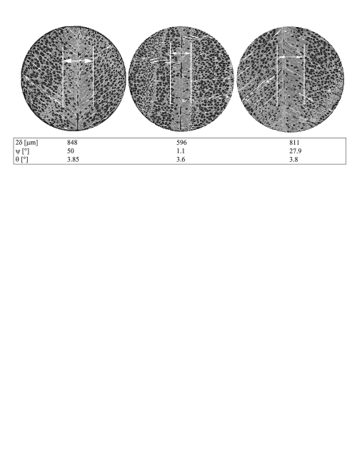
Figure 4: Bond lines with PUR adhesive in beech wood samples. The maximum penetration depth predicted by the model for all samples with growth ring angles $\psi$ and grain angle $\theta$ is shown by the white lines.

• For PUR adhesive, we choose a sample with angles, $\psi$$=$$50^{\circ}$ and $\theta$$=$$3.85^{\circ}$. If we calculate the maximum penetration depth using Eq. 32 we obtain a value of $\delta_{h}$$=$$38.5$mm with hardening as limiting factor, however using the volume limitation with Eq. 33 we obtain $\delta_{V}$$=$$848\rm\mu m$. Therefore we can conclude that all the adhesive penetrated before hardening took place, leaving a starved bond line behind (see Fig. 4). Note that the adhesive penetrates both wood pieces, but significantly deeper into on the application side (right side of samples in Fig. 4). Therefore we have to take an average value of $\delta$$=$$424\mu m$ showing good agreement with the experimental data. To test the model for other orientations $\psi,\theta$, we choose a sample with $\psi$$=$$1.1^{\circ}$ and $\theta$$=$$3.6^{\circ}$. This means we use the previous calculation but apply a new rotation matrix $\underline{\underline{M}}$. We obtain a penetration depth of $\delta_{V}$$=$$596\rm\mu m$, $\delta$$=$$298\rm\mu m$ and $\delta_{h}$$=$$1.32\rm mm$. In Fig. 4 the quality of the analytical prediction is shown. We repeat this for angles $\psi$$=$$27.9^{\circ}$ and $\theta$$=$$3.8^{\circ}$ and obtain the penetration depths $\delta_{V}$$=$$811\mu m$, $\delta$$=$$405.5\rm\mu m$ and $\delta_{h}$$=$$23.6\rm mm$ (compare Fig. 4). These tests show that our model is a good approximation for the beech wood structure and therefore we fix the network parameters $a,b,c,d$ for further calculations.

• We exemplify the penetration of PVAC using a sample oriented at angles $\psi$$=$$46.1^{\circ}$ and $\theta$$=$$3.4^{\circ}$ and calculate the maximum penetration depths from Eqs. 32 and 33. We find $\delta_{V}$$=$$851\rm\mu m$, leading to $\delta$$=$$425.5\rm\mu m$ and $\delta_{h}$$=$$80\rm\mu m$. Therefore the maximum penetration depth is limited by the hardening process. In Fig. 5, we show that almost all the adhesive remains in the bond line with only a small quantity of adhesive inside the vessel network.

• For UF we repeat the same procedure as before on a sample with orientation angles $\psi$$=$$37.2^{\circ}$ and $\theta$$=$$4.3^{\circ}$. We find that the penetration depths are $\delta_{V}$$=$$856\rm\mu m$, $\delta$$=$$428\rm\mu m$, and $\delta_{h}$$=$$141\rm\mu m$ and again the penetration of the adhesive is limited by adhesive hardening. Fig. 5 shows the sample with the predicted penetration depth, exhibiting excellent agreements between the analytical prediction and the experiments.

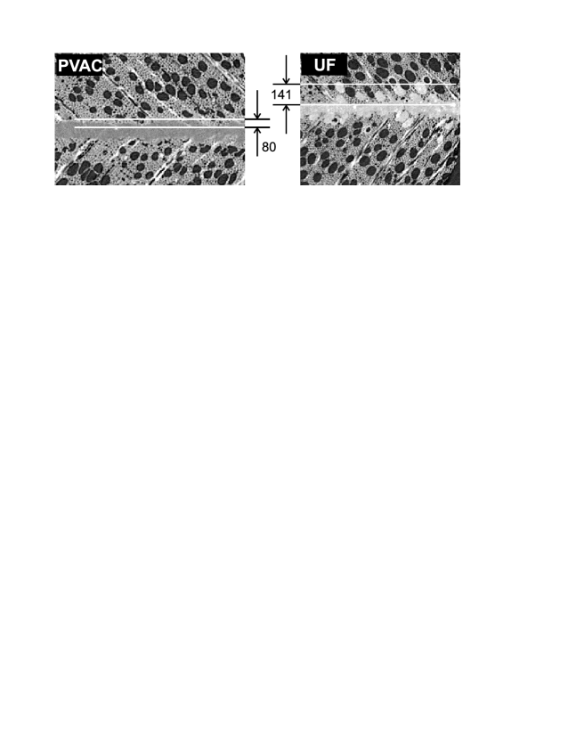
Figure 5: Bond lines of PVAC and UF adhesive in beech wood with maximum predicted penetration depth for samples with the orientation angle $\psi$ and $\theta$. All dimensions are given in $\rm\mu$m.

To study the dependence of maximum penetration depth on the growth ring angle, we take the values for UF and keep all parameters fixed, except the growth ring angle. In Fig. 6 we see the two limiting conditions for the penetration depth. The penetration depth is an increasing function of the growth ring angle for the hardening limitation case, and we observe a distinct maximum at approximately $48$^∘ in the case when the maximum available volume is the limitation. This observation is in agreement with PUR adhesive that fulfills the volume limiting condition, as demonstrated in part I of this work part1 . This result shows that even though we reduce the wood anatomy to a homogeneous, regular network, adhesive transport, the beech wood seems well described by the model and for a desired penetration depth, the model can predict the optimal growth ring angle of the samples.

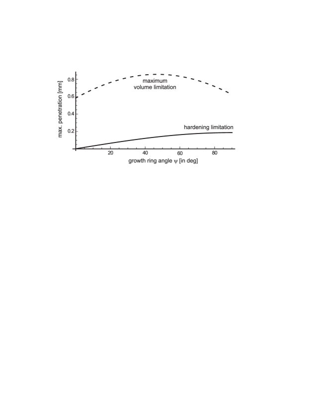
Figure 6: Dependence of the penetration depth on the growth ring angle.

Our model can also be used to design new adhesives with optimized properties, like reactivity, if an ideal penetration depth is to be reached. Fig. 7 shows the maximum penetration depth for a wide range of adhesive parameters $\nu_{1},...,\nu_{4}$ from Fig. 3. We show this in four plots combining two parameters. Horizontal planes represent the case where all available adhesive is inside the vessel structure, while the curved surfaces show the penetration limit due to adhesive hardening. The intersection line (see Fig. 7) separates regions with complete penetration from those, where penetration is limited by adhesive hardening. Therefore, Fig. 7 allows to choose a pair of reactivity parameters in order to obtain a desired penetration depth. The model can also be used to minimize solvent concentration and amount of applied adhesive for a required penetration depth. Fig. 8 illustrates the maximum penetration depth as function of the solvent concentration and the total amount of applied adhesive. The solid lines represent the proportions between solvent concentration and the total applied volume of adhesive which give the same penetration depth.

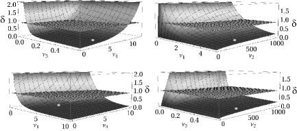
Figure 7: Penetration depth $\delta$ in mm as function of adhesive parameters from Fig. 3 for UF and growth ring angle of 45^∘. The experimentally obtained value for UF is marked with the white dot. (Color version online)

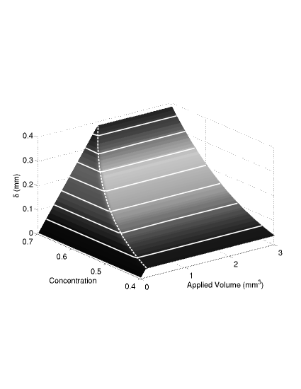
Figure 8: Penetration depth $\delta$ in mm as function of solvent concentration and total amount of applied adhesive for UF and growth ring angle of 45^∘. The solid lines represent the fixed $\delta$ and the dashed line divides the surface into two regions, the right one when the penetration is limited by the hardening process and the left one, when the total volume of applied adhesive is the limiting factor. (Color version online)

4 Discussions and Conclusions

We presented an analytical model for the prediction of the penetration depth of adhesives, paint or hardening fluids in general, into the beech wood structure. Since we focused on hard wood, the pore space of wood is formed by a network of interconnected vessels. The network is characterized by parameters that are related to amplitude and wavelength of the oscillating vessels in tangential and radial direction and the porosity of wood originating from the vessel network. We compared the model to experiments and found good agreement for various adhesives. Therefore, even though we reduce the wood anatomy to a homogeneous, regular network, adhesive transport for the much more disordered, complex pore space of real beech wood seems well described.

The analytical model considers generic types of adhesive hardening. However if other special fluids are to be considered, only the viscosity dependence on concentration and time need to be known. We applied the model to three major types of adhesive which are PUR, UF, and PVAC and compared the respective penetration depths. For adhesives whose hardening process depends on the change of concentration, we include a description for solvent concentration diffusion inside the beech wood. This approach makes the model applicable for adhesives like UF and PVAC. Penetration is limited by two things: the penetration due to the applied pressure that is arrested by hardening processes, and the total amount of applied adhesive that is available to penetrate into the vessel network. The smaller penetration depth is the limiting one. By comparing the model with the experimental data we showed that it is possible to model the maximum penetration depth for three different used adhesives, namely PUR, PVAC, and UF.

Our model is sufficiently simple to allow for a broad applicability. By determining the morphological and rheological parameters, it can be applied to a wide range of wood species and to fluids with various hardening kinematics to predict the penetration depth of these fluids into porous structures, when transport is dominated by capillarity.

References

- (1) A.A. Marra, Technology of wood bonding, Van Nostrand Reinhold, New York, NY (1992).
- (2) J. Custodio, J. Broughton, H. Cruz, A review of factors influencing the durability of structural bonded timber joints, International Journal of Adhesion and Adhesives, 29, 173-185 (2009).
- (3) W.Q. Wang, N. Yan, Characterizing liquid resin penetration in wood using a mercury intrusion porosimeter, Wood and Fiber Science, 37, 505-514 (2005).
- (4) F.A. Kamke, J.N. Lee, Adhesive Penetration of Wood - A Review, Wood and Fiber Science, 39(2), 205-220 (2007).
- (5) J.F. Siau, Transport processes in wood. Springer, New York, NY (1984).
- (6) P. Hass, F.K. Wittel, S.A. McDonald, F. Marone, M. Stampanoni, H.J. Herrmann, P. Niemz, Pore space analysis of beech wood - the vessel network. Submitted to Holzforschung. Preprint visible in electronic form.
- (7) M. Sernek, J. Resnik, and F.A. Kamke, Penetration of liquid Urea-Formaldehyde Adhesive into Beech Wood, Wood and Fiber Science, 31(1), 41-48 (1999).
- (8) P. Niemz, D. Mannes, E. Lehmann, P. Vontobel, and S. Haase, Untersuchungen zur Verteilung des Klebstoffes im Bereich der Leimfugen mittels Neutronenradiographie und Mikroskopie, European Journal of Wood and Wood Products 62, 424-432 (2004).
- (9) B.M. Collett, A Review of Surface and Interfacial Adhesion in Wood Science and Related Fields, Wood Science and Technology, 6,1-42 (1972).
- (10) O. Suchsland, Über das Eindringen des Leims bei der Holzverleimung und die Bedeutung der Eindringtiefe für die Fugenfestigkeit, European Journal of Wood and Wood Products 16(39),101-108 (1958).
- (11) P. Hass, M. Mendoza, F.K. Wittel, P. Niemz, H.J. Herrmann, Adhesive Penetration of Hard Wood: Part I: Experiments on Beech, Submitted to Wood Science and Technology. Preprint visible in electronic form.
- (12) E.W. Washburn, The Dynamics of Capillarity Flow, Phys. Rev. 17, 273-283 (1921).
- (13) H.H. Bosshard, L. Kucera, The Network of Vessel System in Fagus sylvatica L., European Journal of Wood and Wood Products 31,437-445 (1973).
- (14) A. Bhattacharya and P. Ray, Studies on Surface Tension of Poly(Vinyl Alcohol): Effect of Concentration, Temperature, and Addition of Chaotropic Agents, J. of Appl. Poly. Science, 93, 122-130 (2004).
- (15) C.-Y. Hse, Surface tension of phenol-formaldehyde wood adhesives, Holzforschung 26, 82-85 (1972).
- (16) S. Lee, T.F. Shupe, L.H. Groom and C.Y. Hse, Wetting Behaviors of Phenol- and Urea-Formaldehyde Resins as Compatibilizers, Wood and Fiber Science 39, 482-492 (2007).
- (17) S. Kurjatko and J. Kudela, Wood Structure and Properties, Arbora Publisher (1998).
- (18) W. Olek, P. Perré and J. Weres, Inverse analysis of the transient bound water diffusion in wood, Holzforschung 59, 38-45 (2005).