Detectability of large-scale power suppression in the galaxy distribution

Abstract

Suppression in primordial power on the Universe’s largest observable scales has been invoked as a possible explanation for large-angle observations in the cosmic microwave background, and is allowed or predicted by some inflationary models. Here we investigate the extent to which such a suppression could be confirmed by the upcoming large-volume redshift surveys. For definiteness, we study a simple parametric model of suppression that improves the fit of the vanilla $\Lambda$CDM model to the angular correlation function measured by WMAP in cut-sky maps, and at the same time improves the fit to the angular power spectrum inferred from the maximum-likelihood analysis presented by the WMAP team. We find that the missing power at large scales, favored by WMAP observations within the context of this model, will be difficult but not impossible to rule out with a galaxy redshift survey with large volume ($\sim 100~{}{\rm Gpc}^{3}$). A key requirement for success in ruling out power suppression will be having redshifts of most galaxies detected in the imaging survey.

I Introduction

Measurements of the angular power spectrum of the cosmic microwave background (CMB) anisotropies from the WMAP experiment have been used to constrain the standard cosmological parameters to unprecedented accuracy Spergel2003 ; Spergel2006 ; wmap5 ; wmap7 . At the same time, several anomalies have been observed, one of which is the missing power above 60 degrees on the sky in the maps where the galactic plane has been masked Spergel2003 ; wmap123 ; wmap12345 . This is unexpected not only because skies with such lack of large-scale power are expected with the probability of about 0.03% in the standard Gaussian, isotropic model wmap123 ; wmap12345 ; Sarkar , but for two other reasons. First, the missing power occurs on the largest observable scales, where a cosmological origin is arguably most likely. Second, missing correlations are inferred from cut-sky (i.e. masked) maps of the CMB, which makes the results insensitive to assumptions about what lies behind the cut. For review of the missing correlations (and other so-called “large-angle anomalies” in the CMB), see CHSS_review ; for debate on this issue, see CHSS_review ; Efstathiou2009 ; Pontzen_Peiris ; Aurich_Lustig ; for signatures of the anomalies in future polarization observations, see Dvorkin .

In this paper we study the possibility that the primordial power spectrum is suppressed at large scales. This explanation has been invoked before in order to explain the low power in the multipole spectrum (e.g. Contaldi ). In the meantime, observations have made it apparent that the harmonic-space quadrupole and octopole are only moderately low (e.g. O'Dwyer2004 ; Hinshaw:2006ia ), and it is really a range of low multipoles that conspire to produce the vanishing $C(\theta)$. Specifically, as discussed in wmap12345 , there is a cancellation between the combined contributions of $C_{2}$,…,$C_{5}$ and the contributions of $C_{\ell}$ with $\ell\geq 6$. It is this conspiracy that is most disturbing, since it violates the independence of the $C_{\ell}$ of different $\ell$ that defines statistical isotropy.

Note however that it is a priori not at all clear that suppression in the large-scale power can explain the WMAP observations on large scales. While the missing large-angle correlations in the angular two-point correlation function of the CMB $C(\theta)$ could be trivially explained by the missing primordial power, a large suppression would lower the harmonic power spectrum $C_{\ell}$, inferred using the maximum-likelihood estimator, too much to be consistent with observations. [We discuss this in Sections IV and V below.]

In this paper we perform a two-pronged analysis. First, we adopt a simple parametric model for the suppression, and perform a detailed analysis to find the suppressed power spectrum that improves the fit of the vanilla $\Lambda$CDM model to the angular correlation function measured by WMAP in cut-sky maps, and at the same time improves the fit to the angular power spectrum inferred from the maximum-likelihood analysis presented by the WMAP team. Second, we address the following question: if the CMB observations are telling us that the three-dimensional primordial power spectrum is indeed suppressed at large scales (and our adopted model for the suppression is at work), could this effect be confirmed in redshift surveys, with observations of suppressed clustering of galaxies on the largest scales?

It is important to note that we do not concern ourselves with questions recently discussed in the literature as to whether the full-sky or the cut-sky measurements are more robust. It could be the case that one of these measurements, full-sky or cut-sky, is correct while the other is not due to some type of systematic error; it could also be that both of these measurements are correct (in which case the assumption of statistical isotropy is arguably on less firm footing). We consider these possibilities separately in order to get a rough idea on what scale the data favor power suppression in either case. Regardless of which of these possibilities is true, however, our results regarding the detectability of power suppresion, presented in Sec. VI, are valid.

The paper is organized as follows. In Sec. II we do a preliminary investigation in which we attempt to reconstruct the suppression of the primordial power spectrum (and, correspondingly, the matter power spectrum) directly from CMB angular power spectrum measurements (the $C_{\ell}$). In Sec. III, we take the complementary approach, parameterizing the suppression and finding how it affects the $C_{\ell}$ and $C(\theta)$. Sec. IV quantifies how well a given suppressed model fits CMB data in both $C_{\ell}$ and $C(\theta)$. Sec. V provides a discussion of the results that we obtain from this analysis; we find that large-scale suppression of power can significantly increase the likelihood of the observed CMB at large scales. Finally, in Sec. VI, we discuss the possibility of detecting suppression in the matter power spectrum with an upcoming large-volume redshift survey. We conclude in Sec. VII.

II Suppressed power: preliminary investigations

Let us first review the basic way in which the primordial power spectrum determines fluctuations in the CMB observed today. The CMB temperature anisotropies are decomposed into spherical harmonics with coefficients $a_{\ell m}$

$$\frac{\Delta T}{T}(\theta,\phi)=\sum_{\ell=2}^{\infty}\sum_{m=-\ell}^{\ell}a_{\ell m}Y_{\ell m}(\theta,\phi),$$ (1)

where $T$ is the average temperature of the CMB. The angular power spectrum, which quantifies the contribution to the variance of the temperature fluctuations at each $\ell$, is then given by the coefficients $C_{\ell}$ where, assuming statistical isotropy, $\left\langle a_{\ell m}a_{\ell^{\prime}m^{\prime}}\right\rangle=C_{\ell}\delta_{\ell\ell^{\prime}}\delta_{mm^{\prime}}$. We will also consider the angular two-point correlation function

$$C(\theta)\equiv\left\langle\frac{\Delta T}{T}(\hat{n})\frac{\Delta T}{T}(\hat{n}^{\prime})\right\rangle_{\hat{n}\cdot\hat{n}^{\prime}=\cos\theta},$$ (2)

where we have assumed statistical isotropy, and the expectation is taken over the ensemble of universes. $C(\theta)$ is related to the anisotropy power spectrum by

$$C(\theta)=\frac{1}{4\pi}\sum_{\ell=2}^{\infty}(2\ell+1)C_{\ell}P_{\ell}(\cos\theta).$$ (3)

The angular power spectrum $C_{\ell}$ is directly related to the primordial power spectrum of curvature perturbations laid down by inflation. The $C_{\ell}$ are given in terms of the primordial power spectrum by

$$\frac{\ell(\ell+1)C_{\ell}}{2\pi}=\int d(\ln k)\left[T_{\ell}(k)\right]^{2}\Delta_{R}^{2}(k),$$ (4)

where $T_{\ell}(k)$ is the transfer function and $\Delta_{R}^{2}(k)$ is the dimensionless curvature power spectrum

$$\Delta_{R}^{2}(k)\equiv\frac{k^{3}P_{R}(k)}{2\pi^{2}},$$ (5)

where $P_{R}(k)$ is the curvature power spectrum which, at late times and on subhorizon scales, is related to the matter density power spectrum $P(k)$ via $P_{R}(k)\propto k^{-4}P(k)$.

We would like to infer the primordial curvature power spectrum $\Delta^{2}_{R}(k)$ given the angular power spectrum $C_{\ell}$ measured from the CMB. There are two approaches we could take to dealing with Eq. (4): the inverse problem (discussed in this section) and the parametric forward problem of starting with various power spectra and attempting to fit the $C_{\ell}$ (discussed in the next section and pursued in the rest of the paper).

The first option is to directly calculate $\Delta^{2}_{R}(k)$ from the measured angular power spectrum $C_{\ell}$. This inverse problem, where we know the result of the integration but not the integrand, is difficult because the primordial power spectrum $\Delta_{R}^{2}(k)$ is a three-dimensional quantity while the CMB angular power spectrum $C_{\ell}$ is a two-dimensional, projected quantity. When the problem is discretized, as described below, it becomes clear that the problem is underdetermined and ill-conditioned, as is typical for inverse problems: small changes in the observed $C_{\ell}$ typically lead to large changes in the inferred $\Delta^{2}_{R}(k)$.

Since we are examining the phenomenon of low power on large angles in the CMB, it is really the $C(\theta)$ data that we wish to be faithful to, so we take $C(\theta)$ as our starting point rather than $C_{\ell}$. We start from the pixel-based measurement of the angular correlation function (adopted from Sarkar ), which we denote with a tilde, $\tilde{C}(\theta)$. In order to smooth out the noise in the measured $\tilde{C}(\theta)$, and thereby simplify the inverse problem somewhat, we use a “smoothed model” for $\tilde{C}(\theta)$ that is designed to agree with $\Lambda$CDM at small angular scales while closely matching the actual WMAP data at larger angular scales. To this end, we take the $\Lambda$CDM $C(\theta)$ and modify it so that it smoothly transitions to zero for $\theta$ above roughly 60 degrees (Figure 1).

Inverting Eq. (3), we can determine the angular power spectrum coefficients $\tilde{C}_{\ell}$ inferred from our (smoothed) pixel-based estimate $\tilde{C}(\theta)$

$$\tilde{C}_{\ell}=2\pi\int_{-1}^{1}P_{\ell}(\cos\theta)\tilde{C}(\theta)d(\cos\theta).$$ (6)

We are now in a position to directly address the inverse problem in Eq. (5). We solve this numerically by discretizing the integral

$$\frac{\ell(\ell+1)\tilde{C}_{\ell}}{2\pi} = \int d(\ln k)\left[T_{\ell}(k)\right]^{2}\Delta_{R}^{2}(k)$$ (7)

$$\equiv \sum_{k}F_{\ell k}\Delta_{R}^{2}(k).$$ (8)

The kernel $F_{\ell k}$ is extracted from CAMB CAMB . The basic strategy here, distilled in diagrammatic form, is to start from $\tilde{C}(\theta)$ to find the corresponding $\Delta_{R}^{2}(k)$:

$$\tilde{C}(\theta)\rightarrow\tilde{C}_{\ell}\rightarrow\Delta_{R}^{2}(k).$$ (9)

We attempted two different methods of solving this inverse problem, explained more fully in Appendix A. Both methods give similar results, shown with a sample reconstruction in Fig. 9 in the Appendix. While this result can only be suggestive (given that we used a smoothed model for $\tilde{C}(\theta)$ and given that the inverse problem is ill-conditioned and underdetermined), it does indicate that a transition to low/zero power on large angular scales in $\tilde{C}(\theta)$ can be explained by suppression at low $k$ in the primordial power spectrum $\Delta_{R}^{2}(k)$. If the transition to zero power in $\tilde{C}(\theta)$ occurs at about 60 degrees, as it appears to do in the WMAP cut-sky data, then this corresponds to power suppression at scales of $k\lesssim 10^{-3.6}{\rm Mpc}^{-1}\approx 3.5\times 10^{-4}h/{\rm Mpc}$.

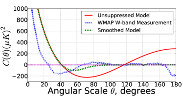
Figure 1: The angular two-point function $C(\theta)$. Measurement from the W-band WMAP 7-year maps, adopted from Sarkar , is shown here in blue, while our model in which $C(\theta)$ smoothly transitions to zero at higher $\theta$ is shown in green. This smoothed model mimics and idealizes the behavior of the measured $C(\theta)$ at large scales but follows the $\Lambda$CDM prediction (red curve) on smaller scales, below roughly 50 degrees. The dotted line shows zero correlation for reference.

III Suppressed primordial large-scale power

The inverse approach from the previous section and the Appendix shows that the direct inversion of our smoothed $C(\theta)$ leads to a suppression of $P(k)$ at $\log_{10}(k_{c}/(h/{\rm Mpc}))\lesssim-3.5$, but the inversion is very noisy and non-robust, as expected. We now change tactics and move to the alternative approach to Eq. (4). Instead of treating this as an inverse problem, we now parameterize $\Delta_{R}^{2}(k)$ and treat this as a (much more stable) forward problem. We utilize a three-parameter model parameterizing the suppressed $\Delta_{R}^{2}(k)$ with an exponential cutoff: following Contaldi and Mort_Hu_pklow , we write

$$\Delta_{R,{\rm sup}}^{2}(k) = \left[1-\beta e^{-(k/k_{c})^{\alpha}}\right]A_{s}(k/k_{0})^{n_{s}-1}$$ (10)

$$\equiv S(k;k_{c},\alpha,\beta)\Delta_{R,{\rm unsup}}^{2}(k),$$ (11)

where we have implicitly defined the factor $S(k;k_{c},\alpha,\beta)\equiv 1-\beta\exp(-(k/k_{c})^{\alpha})$ by which the power spectrum is suppressed. The parameter $k_{c}$ controls the $k$-value of the transition; $\alpha$ controls the sharpness of the transition; and the extra parameter $\beta$, which is not found in Contaldi or Mort_Hu_pklow , allows the power spectrum to plateau to a value other than zero at low $k$ ($S(k)\rightarrow 1-\beta$ for $k\rightarrow 0$). Note that this parameterization has enough freedom to mimic the results of the inversion shown in Fig. 9 almost perfectly.

For a given set of parameters $\{k_{c},\alpha,\beta\}$, we have a well-defined $\Delta_{R}^{2}(k)$ and can thus use the numerical kernel $F_{\ell k}$ to find the corresponding $C_{\ell}$’s, as in Eq. (8). We can then determine which combinations of parameters give $C_{\ell}$’s that fit the observed WMAP $C_{\ell}$’s, and likewise the observed $C(\theta)$. We are now moving in a direction opposite the one in Eq. (9):

$$\Delta_{R}^{2}(k)\rightarrow C_{\ell}\rightarrow C(\theta).$$ (12)

Plots of the suppression factor $S(k)$ for several sample parameter values are shown in Figure 2.

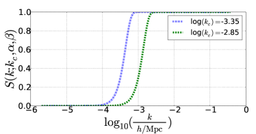
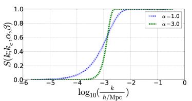
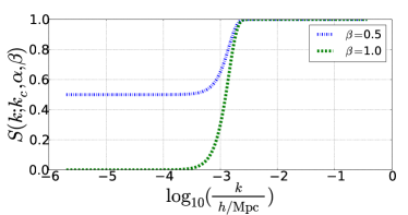
Figure 2: Illustration of what the suppression factor $S(k)$ looks like for various combinations of parameters. The default parameters are $\log(k_{c})\equiv\log_{10}(k_{c}/(h/{\rm Mpc}))=-2.85$, $\alpha=3.0$, and $\beta=1.0$. In each plot, one of these parameters is varied, while the other two are held fixed at their default values.

When varying the suppression parameter $k_{c}$ (and, optionally, $\alpha$ and $\beta$), we have not simultaneously varied other parameters that describe the primordial power spectrum, such as the dark matter and baryon densities, spectral index, etc. The reason, in addition to simplicity, is that none of these other parameters can mimic the large-scale suppression of power, and therefore, power suppression is not degenerate with other cosmological parameters. The one possible exception would be primordial nongaussianity of the local type, which does indeed affect the power spectrum of halos (and, thus, galaxies) on large scales Dalal ; however, including this degeneracy is beyond the scope of this project.

IV Statistical tests

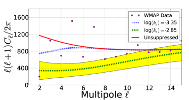
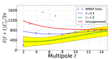
Figure 3: Effects of the suppression on the angular power spectrum $C_{\ell}$. The default parameters are again $\log(k_{c})\equiv\log_{10}(k_{c}/(h/{\rm Mpc}))=-2.85$, $\alpha=3.0$, and $\beta=1.0$. In each panel, one of these parameters is varied, while the other two are held fixed at their default values. The WMAP measurements are shown as points with measurement error bars (too small to see in this plot). Cosmic variance (assuming full-sky measurements) is plotted as a band around the most heavily suppressed model (green curve) in each panel.

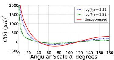
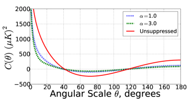
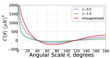
Figure 4: Effects of the suppression on the real-space two-point correlation function in the CMB, $C(\theta)$. The default parameters are again $\log(k_{c})\equiv\log_{10}(k_{c}/(h/{\rm Mpc}))=-2.85$, $\alpha=3.0$, and $\beta=1.0$. In each plot, one of these parameters is varied, while the other two are held fixed at their default values.

We are interested in how a suppressed primordial power spectrum, as given in Eq. (11), affects both $C_{\ell}$ and $C(\theta)$. Figures 3 and 4 show examples of how these quantities vary with changes in the parameters.

More specifically, we look to quantify whether, and to what extent, a suppressed primordial power spectrum gives a better fit to observations of $C_{\ell}$ (typically inferred using maximum-likelihood-type techniques at large scales) and $C(\theta)$ estimated on cut-sky maps using a pixel-based estimator. We restrict attention here to varying $k_{c}$ rather than all three parameters, since variations in $k_{c}$ have the greatest effects on the likelihood, and also since $k_{c}$ directly controls the scale at which the suppression occurs.

In the case of $C_{\ell}$, it is relatively straightforward to quantify the fit between a given suppressed model and the WMAP data. We simply generate a suppressed model using CAMB and then feed the resulting $C_{\ell}$ spectrum into the WMAP likelihood code to obtain a goodness-of-fit criterion. Further details are covered in Sec. IV.1.

Quantifying the fit between a suppressed-model $C(\theta)$ and the WMAP data requires a bit more work. In Sec. IV.2, we examine the statistic $S_{1/2}$, which gives a measure of correlations in the CMB above scales of $60\hbox{${}^{\circ}$}$. In analogy to our treatment of the angular power spectrum, we define a $\chi^{2}$ statistic to quantify the goodness of fit between a given suppressed model and the WMAP data.

IV.1 Angular Power Spectrum $C_{\ell}$

To quantify how well the suppressed angular power spectrum $C_{\ell,{\rm sup}}$ fits the WMAP observations $C_{\ell,{\rm WMAP}}$, we use the WMAP likelihood code to compute $\chi^{2}_{C_{\ell},\rm sup}(k_{c})=-2\ln\mathcal{L}_{\rm sup}(k_{c})$ from $C_{\ell,{\rm sup}}$. We likewise compute $\chi^{2}_{C_{\ell},\rm unsup}=-2\ln\mathcal{L}_{\rm unsup}$ from the unsuppressed $\Lambda$CDM power spectrum $C_{\ell,{\rm unsup}}$, finding the difference

$$\Delta\chi^{2}_{C_{\ell}}(k_{c})=\chi^{2}_{C_{\ell},\rm sup}(k_{c})-\chi^{2}_{C_{\ell},\rm unsup}$$ (13)

as a final quantification of how well the suppressed model fits $C_{\ell}$ data relative to the unsuppressed $\Lambda$CDM model.

A negative $\Delta\chi^{2}_{C_{\ell}}$ indicates that the suppressed model is a better fit to the WMAP data than $\Lambda$CDM . For models with a large amount of suppression (i.e., high $k_{c}$), the suppressed model affects the $C_{\ell}$ at increasingly smaller scales (higher $\ell$), making them inconsistent with the $C_{\ell}$ measured from WMAP and thus making the quantity $\Delta\chi^{2}_{C_{\ell}}$ large and positive.

The results are shown further below in Fig. 6, with discussion in Section V.

IV.2 Angular Correlation Function $C(\theta)$

We now study to what extent the power suppression from our model can account for the low correlations observed above $60\hbox{${}^{\circ}$}$ on the cut-sky WMAP maps Spergel2003 ; wmap123 ; wmap12345 . The statistic $S_{1/2}$, defined in Spergel2003 , quantifies the lack of correlation above 60 degrees

$$S_{1/2}\equiv\int_{-1}^{1/2}\left[C(\theta)\right]^{2}d(\cos\theta).$$ (14)

It is possible to calculate $S_{1/2}$ directly from the $C_{\ell}$’s:

$$S_{1/2}={1\over(4\pi)^{2}}\sum_{\ell,\ell^{\prime}}(2\ell+1)(2\ell^{\prime}+1)C_{\ell}I_{\ell,\ell^{\prime}}(1/2)C_{\ell^{\prime}}.$$ (15)

For details of how the quantity $I_{\ell,\ell^{\prime}}$ is calculated, see Appendix A of the published version of Ref. wmap12345 .

We would like to generate statistical realizations of the angular power spectrum based on the underlying primordial power spectrum $\Delta_{R}^{2}$. To do that, we first calculate the expected angular power spectrum $C_{\ell,{\rm original}}$ (using Eq. (7)), and then create realizations using

$$C_{\ell,{\rm realization}}=fC_{\ell,{\rm original}}$$ (16)

where the multiplicative factor

$$f=\frac{\Gamma(k=(2\ell+1)f_{\rm sky}/2,\theta=2)}{(2\ell+1)f_{\rm sky}}:$$ (17)

the numerator is drawn from a gamma distribution with scale parameter $\theta=2$ and shape parameter $k=(2\ell+1)f_{\rm sky}/2$, and the denominator ensures that the mean of $f$ is unity. The reason we draw from a gamma distribution is that this is the appropriate generalization of a $\chi^{2}$ distribution when the number of degrees of freedom is non-integer, as it is above for $f_{\rm sky}\neq 1$; $\Gamma(k=r/2,\theta=2)$ is identical to a $\chi^{2}$ distribution for integer $r$ degrees of freedom. We adopt $f_{\rm sky}=0.75$ for the remainder of this paper. [Modeling of the noise is unnecessary since cosmic variance dominates at these large scales.]

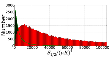
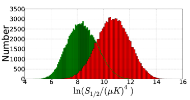
Figure 5: The distribution of our realizations of the statistic $S_{1/2}$ for the unsuppressed (red histograms) and a sample suppressed (green histograms) model. The suppressed model has $\log_{10}(k_{c}/(h/{\rm Mpc}))=-2.85$, $\alpha=3.0$, and $\beta=1.0$, and has a better fit than the unsuppressed model by $\Delta\chi^{2}_{S_{1/2}}=-7.9$. The bottom panel clearly shows that the distribution of $S_{1/2}$ is lognormal, whether or not the underlying power spectrum is suppressed.

We examine the resulting distribution of $S_{1/2}$ values by performing 100,000 realizations of the $C_{\ell}$ for $2\leq\ell\leq 50$ (going to higher values of $\ell$ barely changes the $S_{1/2}$ statistic, since scales above $60\hbox{${}^{\circ}$}$ are mostly affected by $\ell\lesssim 10$), assuming central values $C_{\ell,{\rm original}}$ calculated based on the suppressed primordial power spectrum as in Eq. (8), and calculating $S_{1/2}$ for each set of $C_{\ell,{\rm realization}}$. We find that $S_{1/2}$ is distributed approximately according to a lognormal distribution, both for suppressed and unsuppressed models, and regardless of the particular value of $k_{c}$. This is illustrated in Fig. 5.

In the sample suppressed model ($\log_{10}(k_{c}/(h/{\rm Mpc}))=-2.85$) shown in Fig. 5, the histogram of $S_{1/2}$ peaks at $1000(\mu K)^{4}$, has a mean of $8300(\mu K)^{4}$, and a median of $4300(\mu K)^{4}$. The histogram of $\ln(S_{1/2})$ peaks at 8.4, corresponding to an $S_{1/2}$ of $4400(\mu K)^{4}$. These values are all much lower than the mean value expected in the best-fit $\Lambda$CDM cosmology (about $50,000(\mu K)^{4}$), but bigger than the value measured in WMAP cut-sky maps (about $1000(\mu K)^{4}$).

In order to calculate a $\chi^{2}$ statistic in analogy to the $\Delta\chi^{2}_{C_{\ell}}$ above, we first transform the lognormal $S_{1/2}$ distribution to a Gaussian by taking the natural log of the $S_{1/2}$ values. The result, a nearly perfect Gaussian, is shown for the unsuppressed and the sample suppressed model in the lower panel of Fig. 5. We can then calculate the $\chi^{2}$ corresponding to the probability of getting a certain value $S_{1/2}^{\rm obs}$ of $S_{1/2}$

$$\chi^{2}_{S_{1/2},{\rm sup}}=\left[\frac{\ln(S_{1/2}(k_{c}))-\ln(S_{1/2}^{\rm obs})}{\sigma_{\ln(S_{1/2})}}\right]^{2}$$ (18)

where $\ln(S_{1/2}(k_{c}))$ is the mean over the realizations of $\ln(S_{1/2})$ for the given $k_{c}$ and $\sigma_{\ln(S_{1/2})}$ is the standard deviation over all realizations. For the purposes of this paper, we choose $S_{1/2}^{\rm obs}=1000\,(\mu$K$)^{4}$, since this is (roughly) the value of $S_{1/2}$ favored by the cut-sky WMAP observations Spergel2003 ; wmap123 ; wmap12345 ; Sarkar .

We also performed 6,500,000 realizations of the $C_{\ell}$ assuming central values $C_{\ell,{\rm original}}$ corresponding to the unsuppressed $\Lambda$CDM model. From the $S_{1/2}$ values associated with these realizations, we calculate $\chi^{2}_{S_{1/2},{\rm unsup}}$ in exact analogy to Eq. (18), and then compute

$$\Delta\chi^{2}_{S_{1/2}}(k_{c})=\chi^{2}_{S_{1/2},\rm sup}(k_{c})-\chi^{2}_{S_{1/2},\rm unsup}.$$ (19)

A combined statistic that takes into account both the measurements of the angular power spectrum $C_{\ell}$ and the total angular correlation above $60\hbox{${}^{\circ}$}$ parameterized by the statistic $S_{1/2}$, is then given by

$$\mathcal{L}(k_{c}) = \exp\left(-\frac{\Delta\chi^{2}_{C_{\ell}}(k_{c})}{2}\right)\times\exp\left(-\frac{\Delta\chi^{2}_{S_{1/2}}(k_{c})}{2}\right)$$ (20)

$$\equiv P(C_{\ell})\times P(S_{1/2}).$$

Both $P(S_{1/2})$ and $P(C_{\ell})$ are normalized so that their values for the unsuppressed $\Lambda$CDM model are 1. Hence $P(S_{1/2})$ and $P(C_{\ell})$ should be interpreted as the improvement (relative to fiducial unsuppressed $\Lambda$CDM) in how well a given suppressed model fits the WMAP data for $C_{\ell}$ and $S_{1/2}$. Note that we are not taking the correlation between the (maximum-likelihood) $C_{\ell}$ and the (pixel-based) $S_{1/2}$ into account in our statistic $\mathcal{L}(k_{c})$. We define the statistic in the simplest possible way, by multiplying the individual likelihoods in $C_{\ell}$ and $S_{1/2}$. This simple combination is sufficient, since it favors suppression on scales between the scales which $P(S_{1/2})$ and $P(C_{\ell})$ independently prefer (this is confirmed in Fig. 6), and thus captures the essence of how these two quantities jointly favor suppression. Note that the main results of this paper, presented in Sec. VI, do not depend on exactly how we combine the likelihood in the measured full-sky $C_{\ell}$ and cut-sky $S_{1/2}$; we only use $\mathcal{L}(k_{c})$ from Eq. (20) to get a rough idea about the scale at which suppression is favored by the data if both measurements are taken at face value. We then proceed in Sec. VI to study the detectability of suppressed power corresponding to a range of values of the suppression scale $k_{c}$; these results do not depend on how $P(C_{\ell})$ and $P(S_{1/2})$ are combined.

We are now in a position to determine which values of the suppression scale $k_{c}$ improve the joint fit to the angular power spectrum $C_{\ell}$ and the cut-sky measurements of the angular correlation function $C(\theta)$ above $60\hbox{${}^{\circ}$}$ (quantified by the statistic $S_{1/2}$).

V Current constraints from the CMB

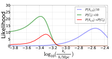
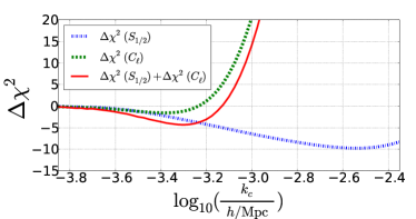
Figure 6: The improvements in $P(S_{1/2})$, $P(C_{\ell})$, and the product thereof – all relative to the unsuppressed model – are plotted as a function of $k_{c}$. The top panel shows $P(S_{1/2})$ divided by 10 and $P(C_{\ell})$ multiplied by 10. The $P(S_{1/2})$ values are based on 100,000 realizations of the $C_{\ell}$’s as described in the text. The bottom panel shows the same information as the top panel, but puts it in terms of chi-square goodness-of-fit statistics. The maximum improvement in $P(S_{1/2})\times P(C_{\ell})$, relative to the unsuppressed $\Lambda$CDM model, is a factor of 8.7 ($\Delta\chi^{2}_{S_{1/2}}+\Delta\chi^{2}_{C_{\ell}}=-4.3$), occurring at $\log_{10}(k_{c}/(h/{\rm Mpc}))\approx-3.3$. All calculations were performed assuming $f_{\rm sky}=0.75$.

The top panel of Fig. 6 shows $P(S_{1/2})$, $P(C_{\ell})$, and their product as a function of $k_{c}$, with $\alpha$ held fixed at 3.0 and $\beta$ held fixed at 1.0. The bottom panel displays the same result using $\chi^{2}_{S_{1/2}}$ and $\chi^{2}_{C_{\ell}}$ on the vertical axis instead of $P(S_{1/2})$ and $P(C_{\ell})$.

As indicated in Fig. 6, introducing suppression in the primordial power spectrum can increase the likelihood of both the observed $C_{\ell}$ and the observed $S_{1/2}$, but these two observations favor suppression at different scales. The likelihood of the $C_{\ell}$ is improved by at most a factor of 2.2, with the improvement peaking at $\log_{10}(k_{c}/(h/{\rm Mpc}))=-3.4$, while greater suppressions can improve the likelihood of the $S_{1/2}$ data by huge factors of up to 131, peaking around $\log_{10}(k_{c}/(h/{\rm Mpc}))=-2.6$ (note the plotting scale of likelihoods in Fig. 6, where individual likelihood curves are divided or multiplied by 10 for visual clarity). The $C_{\ell}$ measurements thus favor suppression on very large scales, while the cut-sky $S_{1/2}$ favor suppression all the way down to relatively small scales, where suppression is overwhelmingly ruled out by $C_{\ell}$ data. This is another reminder of just how low the pixel-based cut-sky measurement of $S_{1/2}$ is. It is also a reminder of the fact that such a low value of $S_{1/2}$ represents a conspiracy of the low-$\ell$ $C_{\ell}$ values: the WMAP cut-sky data indicate that $S_{1/2}$ is sufficiently low as to strongly (by factors of over 100 in likelihood) favor suppression of primordial power at scales corresponding to $k=10^{-2.6}\approx 0.003\,h/{\rm Mpc}$, even though the maximum-likelihood $C_{\ell}$ favor suppression only weakly, at far larger scales, and overwhelmingly reject the possibility of suppression at the scales favored by the cut-sky $S_{1/2}$. A sky with such a low $S_{1/2}$ as the WMAP cut sky ought to have $C_{\ell}$’s that are even more suppressed than the most suppressed model in Fig. 3. What we see instead are low-$\ell$ $C_{\ell}$ values that are not so close to zero, but which instead conspire with one another in just such a manner as to produce an exceptionally low value of $S_{1/2}$ anyway wmap12345 .

In any case, we have calculated the product statistic $\mathcal{L}(k_{c})=P(S_{1/2})\times P(C_{\ell})$, or alternatively $\Delta\chi^{2}_{S_{1/2}}+\Delta\chi^{2}_{C_{\ell}}$, as a measure of how well a given suppressed model fits the WMAP data in both $C_{\ell}$ and $C(\theta)$ (the latter via the specific statistic $S_{1/2}$). Since $C_{\ell}$ and $S_{1/2}$ data favor suppression at such different scales, there should be a “sweet spot” somewhere between the peak in $P(C_{\ell})$ and the peak in $P(S_{1/2})$, where suppression is moderately favored by both $C_{\ell}$ and $S_{1/2}$, or heavily favored by one and still allowed by the other. This is indeed what we find, as indicated by the red curve in Fig. 6. Because suppression on overly small scales (below $\log_{10}(k_{c}/(h/{\rm Mpc}))\sim-3.2$) brings the $C_{\ell}$ data for the suppressed model into severe conflict with the WMAP $C_{\ell}$’s, the peak of the $\mathcal{L}$ curve occurs above these scales, even in spite of the huge gains in likelihood that $P(S_{1/2})$ gives us at much smaller scales, where the gain in $P(S_{1/2})$ is still substantial and the $C_{\ell}$ data still favor – or at least do not heavily disfavor – suppression. The maximum improvement possible in $P(S_{1/2})\times P(C_{\ell})$, relative to the unsuppressed $\Lambda$CDM model, is a factor of 8.7 ($\Delta\chi^{2}_{S_{1/2}}+\Delta\chi^{2}_{C_{\ell}}=-4.3$), occurring at $\log_{10}(k_{c}/(h/{\rm Mpc}))\approx-3.3$.

The WMAP likelihood code uses a Bayesian (Gibbs sampler) maximum likelihood method (e.g. Efstathiou2003 ) to compute the fiducial $C_{\ell}$’s at the multipoles $\ell\leq 32$ Dunkley_wmap5 ; Larson_wmap7 . We experimented with running the likelihood code using pseudo-$C_{\ell}$ estimates at low multipoles and discovered that in this case, suppression is much more heavily favored by the $C_{\ell}$ likelihood than it is in the (presumably more accurate) Gibbs sampler, or else a similar Maximum Likelihood Estimate (MLE) method. This result is expected, and holds because the $C_{\ell}$’s that result from the pseudo-$C_{\ell}$ estimates are lower than those found using the Gibbs sampler method (see e.g. Fig. 15 in Hinshaw:2006ia ), and suppression fits them better. In this case we can get $\Delta\chi^{2}_{C_{\ell}}$ as low as $-7.6$, corresponding to improvements in $P(C_{\ell})$ by factors of up to 44 (as opposed to roughly 2 in the best-case scenarios discussed above).

VI Future detectability using galaxy surveys

The results of the previous section indicate that suppression of primordial power on large scales can increase the likelihood of both the observed $C_{\ell}$ angular power spectrum and the observed cut-sky value of $S_{1/2}$, provided the suppression “kicks in” on appropriate scales. Now we turn to the question of whether large-scale suppressed power could be detected in the matter power spectrum as measured by upcoming redshift surveys such as the Large Synoptic Survey Telescope (LSST; LSST ). If the zero-correlation signature of large-angle $C(\theta)$ in the CMB is an authentic effect indicating a deficit of power on the Universe’s largest scales, is it possible to cross-check and verify this result using large-scale-structure data?

Given suppression of the primordial power spectrum $\Delta_{R}^{2}(k)$ as parameterized in Eq. (11), the matter power spectrum will be suppressed by the same factor as $\Delta_{R}^{2}(k)$:

$$P_{\rm sup}(k)=S(k)P_{\rm unsup}(k)$$ (21)

where $S(k)\equiv S(k;k_{c},\alpha,\beta)$ is the same as before. We wish to determine whether this suppressed matter power spectrum could be distinguished from the unsuppressed $\Lambda$CDM matter power spectrum $P_{\rm unsup}(k)$ by a large-volume redshift survey.

When measuring the matter power spectrum with a redshift survey, the error bars in each thin slice in redshift $dz$ and wavenumber $dk$ are given by the Feldman-Kaiser-Peacock (FKP; FKP ) formula

$$\sigma_{P}^{2}(k,z)=\frac{4\pi^{2}P(k,z)^{2}}{k^{2}\,dk\,dV_{\rm eff}}$$ (22)

where the effective volume element $dV_{\rm eff}(k,z)$ is related to a comoving volume element via

$$dV_{\rm eff}(k,z)=\left[\frac{n(z)P(k,z)}{1+n(z)P(k,z)}\right]^{2}dV_{\rm survey}(z).$$ (23)

The differential survey volume is given in terms of $dz$ via

$$dV_{\rm survey}=\Omega_{\rm survey}\frac{r(z)^{2}}{H(z)}dz,$$ (24)

where $r(z)$ is the comoving distance as a function of redshift, $H(z)$ is the Hubble parameter as a function of redshift, and $\Omega_{\rm survey}$ is the angular size of the survey in steradians.

The number density of galaxies $n(z)$ can be found from

$$n(z)=m(z)\times\frac{N_{\rm tot}}{\Omega_{\rm survey}\int m(z)[r(z)^{2}/H(z)]dz}$$ (25)

where the second term on the right-hand side provides a normalization. Here $N_{\rm tot}$ is the total number of galaxies in the survey and $m(z)$ is the (unnormalized) number density of galaxies, whose functional form we adopt to be

$$m(z)=\frac{z^{2}e^{-z/z_{0}}}{2z_{0}^{3}}.$$ (26)

We take $z_{0}=0.35$, corresponding to the density roughly expected in the imaging portion of the LSST survey HTBJ , and assume a 23,000 square degree redshift survey with $0.5$, $5$ or $50$ spectra per square arcminute. [Note that the $0.5$ and $5$ gal/arcmin² cases are realistic, being targeted by surveys in the near future BigBoss ; Wang_space , while $50$ gal/arcmin² corresponds to the more aggressive case where spectra of most galaxies in the imaging portion of the survey are taken.]

Given a suppressed power spectrum as in Eq. (21), we can calculate

$$d\chi^{2} \equiv \frac{\left[P_{\rm unsup}(k,z)-P_{\rm sup}(k,z)\right]^{2}}{\sigma_{P}^{2}}$$ (28)

$$= \left[\frac{nP}{1+nP}\right]^{2}\left[\frac{\Omega_{\rm survey}k^{3}}{4\pi^{2}P^{2}}\right]\left[\frac{r^{2}}{H}\right]$$

$$\times\left[P_{\rm unsup}-P_{\rm sup}\right]^{2}d(\ln k)dz$$

and then integrate in order to find the $\chi^{2}$ statistic for how well the survey can distinguish between the suppressed and unsuppressed models.

Note that in the above two equations, wherever a $P\equiv P(k,z)$ occurs without being marked as either suppressed or unsuppressed, this is intended to indicate that either $P_{\rm sup}$ or $P_{\rm unsup}$ may be used. Whether we use $P_{\rm sup}$ or $P_{\rm unsup}$ depends entirely on which question we are trying to answer: If we use suppressed-model error bars, then this $\chi^{2}\equiv\chi^{2}_{\rm sup}$ indicates at what confidence level the survey can rule out suppression. Meanwhile, if we use unsuppressed-model error bars, then $\chi^{2}\equiv\chi^{2}_{\rm unsup}$ indicates at what confidence level the survey can rule out the unsuppressed $\Lambda$CDM model. Ruling out $\Lambda$CDM is considerably more ambitious than ruling out suppression, since the error bars tend to be smaller when they are based on the suppressed model (due to the fact that $\sigma_{P}\propto P+1/n$).

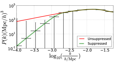
Figure 7: Matter power spectrum $P(k)$ with and without suppression. In the suppressed model, the parameters are $\log_{10}(k_{c}/(h/{\rm Mpc}))=-2.85$, $\alpha=3.0$, and $\beta=1.0$. The power spectrum is shown at $z=0$ for a redshift survey with 50 galaxies per square arcminute. The error bars are based on the suppressed power spectrum, which means that a sufficiently high $\chi^{2}$ value here would indicate the possibility of ruling out suppression. The value of $\chi^{2}$ turns out to be 57.8, good enough to rule out suppression at roughly 7.6$\sigma$. (Bins without vertical error bars contribute nothing to the $\chi^{2}$ – in effect, their error bars are infinite.) Note the log scale on both axes.

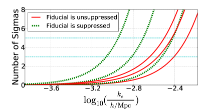
Figure 8: The detectability of suppression as a function of $k_{c}$. These results apply to a survey that extends from $z=0$ to $z=3$ covering 23,000 square degrees of sky. From bottom to top in each set of lines, we assume 0.5, 5 or 50 (spectroscopic) galaxies per square arcminute. [Note that the $0.5$ gal/arcmin² case is entirely realistic in the near future, corresponding to the number density of spectra planned by e.g. BigBoss BigBoss , while $50$ gal/arcmin² corresponds to the more aggressive case where spectra of most galaxies in a large-volume imaging survey are taken.] Here $\alpha$ is fixed at 3.0 and $\beta$ is fixed at 1.0.

This is illustrated in Fig. 7. The plot shows the unsuppressed matter power spectrum, along with the suppressed version for a particular choice of parameters. The goal of calculating $\chi^{2}$ as in Eq. (28) is to determine whether the unsuppressed power spectrum can be distinguished from the suppressed power spectrum for a given set of parameters within the error bars that would be set by an LSST-like survey. For the case pictured – in which the unsuppressed model is taken as true, and the error bars are calculated based on the suppressed model which is being tested – it is possible to rule out suppression with high statistical significance. The opposite is, however, not true: if the suppressed model is true, it will be very difficult to rule out the standard unsuppressed $\Lambda$CDM due to its larger errors.

For example, survey measurements that fell along the curve predicted for the unsuppressed $P(k)$ would, in the case shown in Fig. 7, fall outside some of the suppressed-model error bars, and ultimately combine to give a total $\chi^{2}$ of $57.8$, given the survey parameters outlined in the next paragraph. Meanwhile, taking the unsuppressed model as fiducial would allow for the possibility of survey measurements ruling out $\Lambda$CDM, but the total $\chi^{2}$ would shrink to $2.0$ due to the larger error bars.

The final results for the detectability of suppression are shown in Fig. 8. Instead of plotting $\chi^{2}$ we show the number of sigmas (i.e. $\sqrt{\Delta\chi^{2}}$) at which suppressed and unsuppressed power spectra can be distinguished assuming one degree of freedom on the measurements of $P(k)$. The figure shows the results as a function of $k_{c}$, holding the parameters $\alpha$ and $\beta$ fixed at 3.0 and 1.0, respectively, and assuming three different possible values for the number of galaxies observed per square arcminute ($0.5$, $5$, and $50$) in the spectroscopic survey. We also examined the results with different values of $\alpha$ and $\beta$, but changes in these parameters do not greatly affect the results unless $\beta$ becomes close to zero. The scale of the suppression as determined by $k_{c}$ is by far the greatest contributing factor in determining whether a given suppressed model will be detectable to a large-volume redshift survey.

Comparison of Fig. 8 with Fig. 6 shows that if present data for $C_{\ell}$ and $C(\theta)$ truly point to suppression of the primordial power spectrum, that suppression is likely on scales that are too large for foreseeable redshift surveys to either detect or rule out. The most optimistic scenario shown in Fig. 8, in which there are 50 galaxies per square arcminute in the spectroscopic survey, still cannot (at 3$\sigma$) rule out suppression if $\log_{10}(k_{c}/(h/{\rm Mpc}))\lesssim-3.0$, and cannot rule out $\Lambda$CDM unless the Universe actually shows suppression of the matter power spectrum on much smaller scales, with $\log_{10}(k_{c}/(h/{\rm Mpc}))\gtrsim-2.7$. Suppression on scales this small is strongly disfavored by WMAP $C_{\ell}$ observations. Meanwhile, the scales on which WMAP observations tend to favor suppression ($\log_{10}(k_{c}/(h/{\rm Mpc}))\sim-3.3$) are nearly inaccessible to galaxy surveys. This is a reflection of the fact that the CMB probes much larger scales than even the largest-volume redshift surveys of the near future.

If only the cut-sky $S_{1/2}$ statistic is taken into account, CMB observations heavily favor suppression on scales where suppression would be readily detectable by redshift surveys, at several sigma, for number densities of galaxies expected in near-future spectroscopic samples.

VII Conclusions

In this paper we have studied the suppression of primordial power on large scales as a possible explanation for the CMB observations. Without considering particular physical models for the suppression, we adopted a more pragmatic approach and addressed the following question: do the suppressed models actually improve the likelihood of the observed CMB sky and, if so, can the upcoming large-volume galaxy redshift surveys be used to confirm this suppression?

We first motivated our search by attempting to invert the observations of the angular power spectrum $C_{\ell}$ in order to reconstruct the three-dimensional power spectrum $P(k)$. As expected, this procedure is very unreliable and noisy due to the nature of the inverse problem; nevertheless, we obtained useful hints for the form of the suppression that we should be considering (see Fig. 9 in the Appendix).

We then proceeded to use a parametric model of the suppression (Eq. (11)), with the most important parameter (and the only one we varied in our analysis) being the suppression scale $k_{c}$. We found (see Fig. 6) that the angular power spectrum $C_{\ell}$, traditionally inferred using maximum-likelihood-type estimators, prefers a moderate suppression of power; conversely, the cut-sky pixel-based correlation $C(\theta)$ prefers a stronger suppression. It is also possible that both the full-sky measurement of $C_{\ell}$ and the cut-sky measurement of $C(\theta)$ are not anomalous, but rather that the underlying cosmological model is not statistically isotropic. While it is not clear how to write down the combined likelihood in the full-sky and cut-sky measurements without assuming statistical isotropy, our simple choice (Eq. (20)) prefers the suppression at $\log_{10}(k_{c}/(h/{\rm Mpc}))\approx-3.3$, and increases the combined likelihood by about a factor of 8.7, corresponding to $\Delta\chi^{2}=-4.3$.

Detectability of such a large-scale suppression with future surveys will be difficult, however, as shown in Fig. 8. In order to detect the suppression favored by the CMB angular power spectrum, an LSST-type survey, with a volume of about 100 Gpc³ and a very large number of galaxy redshifts measured, will be necessary. Roughly speaking, a statistically significant ruling-out of the power suppression will require spectra taken of most galaxies in the imaging portion of the survey; this will require a $\sim 10$-meter ground-based, or a $\sim 1.5$-meter space-based, telescope dedicated to taking spectra. Alternatively, photometric redshift techniques may someday become so accurate that our preferred case of “nearly all galaxies being spectroscopic” is validated relatively straightforwardly.

Additionally, we point out that suppressed power will be more easily ruled out (given that the true power is not suppressed) than vice versa, essentially because the model being tested has smaller cosmic-variance errors if it has lower power. Therefore, if indeed we live in the universe with the true power spectrum of density fluctuations being standard inflationary power-law (i.e. unsuppressed), then, for example, a survey covering half the sky with 5 galaxy redshifts per square arcminute will be able to rule out power suppressions on scales above roughly 1 Gpc at 3$\sigma$ confidence; suppression extending to smaller scales is even easier to detect.

Overall, we are optimistic about the prospects of galaxy surveys to test models of the suppressed large-scale power of primordial fluctuations. Dark Energy Survey (DES; des05 ), Baryon Oscillation Spectroscopic Survey (BOSS; boss ) and, especially, very-large-volume surveys such as the LSST LSST , Joint Dark Energy Mission (JDEM; JDEM ), Euclid Euclid , and BigBoss BigBoss , will be able to test, at least in part, observations of CMB experiments on the largest observable scales.

Appendix A Direct inversion to obtain the primordial power spectrum

As pointed out in Sec. II, the CMB angular power spectrum $C_{\ell}$ is given in terms of the primordial power spectrum by

$$\frac{\ell(\ell+1)C_{\ell}}{2\pi} = \int d(\ln k)\left[T_{\ell}(k)\right]^{2}\Delta_{R}^{2}(k)$$ (29)

$$= \sum_{k}F_{\ell k}\Delta_{R}^{2}(k),$$ (30)

where the discretized numerical kernel $F_{\ell k}$ is extracted from CAMB CAMB . Trying to find $\Delta_{R}^{2}(k)$ from a given set of $C_{\ell}$’s (which themselves correspond to a given $C(\theta)$) is an inverse problem, which we attempted to solve using two different strategies. [We also attempted a third, doing a simple matrix inversion of the kernel, but this strategy simply does not work due to the extreme ill-conditioning.] The first is the Richardson-Lucy method, an algorithm that iteratively solves for the portion of the sum that multiplies the kernel nicholson2009reconstruction ; Shafieloo:2003gf ; Shafieloo:2007tk ; Hamann:2009bz :

$$\Delta^{2}_{i+1}(k)=\Delta^{2}_{i}(k)\sum_{\ell=\ell_{\min}}^{\ell_{\max}}\tilde{F}_{\ell k}\frac{C_{\ell}^{obs}}{C_{\ell}^{i}},$$ (31)

where $C_{\ell}^{obs}$ are the observed $C_{\ell}$’s (in this case, the $C_{\ell}$’s corresponding to the smoothed $C(\theta)$ shown as the green curve in Fig. 1), $C_{\ell}^{i}$ is calculated from Eq. (30) for each iteration $i$, and

$$\tilde{F}_{\ell k}=F_{\ell k}/\sum_{\ell}F_{\ell k}.$$ (32)

The method converges to a solution for $\Delta_{R}^{2}(k)$, but has no special properties guaranteeing convergence or smoothness of the solution.

A second strategy makes use of linear regularization, which is one way of putting extra constraints on the solution. The angular power spectrum $C_{\ell}$ is a two-dimensional quantity, while the primordial power spectrum $\Delta^{2}(k)$ is three-dimensional, and so finding the latter from the former is an underdetermined problem. Linear regularization compensates for the fact that the inverse problem is underdetermined.

Numerical Recipes NR outlines one method of regularizing, which favors a constant solution and penalizes deviations from this. The goal here is to solve the equation

$$Ku=b,$$ (33)

where we refer to matrix $K$ as the kernel; $b$ is a known vector; and $u$ is the vector to be solved for. Regularization does this by solving the regularized equation

$$(K^{T}K+\lambda H)u=K^{T}b,$$ (34)

where $H$ is a matrix that takes a different form depending on whether the regularization is linear (penalizing deviations from a constant solution), quadratic, etc., and $\lambda$ is a parameter that controls how strong the regularizing constraint is: higher values of $\lambda$ impose stronger regularizing constraints on the solution. In our case, we take the kernel $K$ to be $F_{\ell k}$, $u$ to be a column vector corresponding to $\Delta_{R}^{2}(k)$, and $b$ to be a column vector corresponding to $C_{\ell}^{obs}$. We adopt $H$ corresponding to linear regularization.

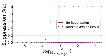
Figure 9: Sample results of the direct inversion. The green points represent the factor $S(k)$ (see definition of $S(k)$ in Eq. (11)) by which the primordial power spectrum $\Delta_{R}^{2}$ is suppressed as determined by the regularized inversion from Eq. (30). The angular power spectrum $C_{\ell}$ used in this inversion corresponds to the $C(\theta)$ shown as the smoothed green curve in Fig. 1, though we could have in principle used the actual WMAP data shown as a blue curve in the same figure.

It is difficult to get consistent results from either of these strategies, given the ill-conditioned and underdetermined nature of the inverse problem. This is part of the reason why we chose to focus most of our attention on doing the forward problem outlined in Eq. (12). However, to the extent that consistent results are possible, both strategies give similar solutions. A sample result for the suppression factor $S(k)$ (see definition of $S(k)$ in Eq. (11)) is shown in Fig. 9.

The most notable feature of the inversion result is that it transitions to near-zero power at large scales/low $k$, with a form suggesting an exponential cutoff; this provides motivation for adopting the form we did for parametrizing $\Delta_{R}^{2}$ in the forward problem (Eq. 11)). Unfortunately, a direct inversion of the sort described in this Appendix requires some fine-tuning in order to get results of this quality, which is why we have emphasized that these results are suggestive rather than conclusive. The results in Fig. 9 (which correspond directly to the regularized inversion, but are also similar to the results of the Richardson-Lucy method) rely on careful tuning of the regularization parameter $\lambda$ to ensure that the result does not become negative at low $k$. [If the regularization is “not strong enough,” with $\lambda$ too small, deviations from a constant solution are not sufficiently penalized to prevent the solution becoming negative. If the regularization is “too strong,” with $\lambda$ too large, the solution simply stays constant at roughly 1. Only in particular intermediate cases does it transition nicely from 0 to 1.]

In addition to this issue, the fact that the inversion results show $S(k)$ of exactly 1 at high $k$ is a result of a mechanism that was put into the solution process by hand. Without enforcing the high-$k$ value, the results often converge to a constant which deviates from unity at high $k$. To compensate for this and for the issue that the solution does not always asymptote to nonnegative values at low $k$, we attempted a modification of the regularized inversion in which deviations from 0 and 1 are penalized (rather than deviations from a constant solution, as in linear regularization). The solutions we obtained using this method have the same general form as shown in Fig. 9, with a transition from 0 to 1 somewhere between $\log_{10}(k_{c}/(h/{\rm Mpc}))=-3$ and $-4$, but the results are even noisier than the results obtained with Richardson-Lucy and linear regularization.

When the WMAP data was used directly as input, rather than the $C_{\ell}$ corresponding to the smoothed model in Fig. 1, solutions to the inverse problem were even noisier.

Finally, neither the regularized inversion nor the Richardson-Lucy method give error bars with which the precision of the inversion might be judged. For all these reasons, the results of the direct inversion cannot be taken as anything more than suggestive. With that caveat, it is still notable that results of both the regularized inversion and Richardson-Lucy method do consistently suggest a transition from suppressed power at low $k$ to unsuppressed power at high $k$. This provides a hint of the fact that the likelihood of the WMAP $C_{\ell}$ and $C(\theta)$ data may be increased by introducing suppression, as explored much more fully, and confirmed, in Sections IV and V.

References

- (1) D. N. Spergel et al. (WMAP), ApJS 148, 175 (2003), astro-ph/0302209
- (2) D. Spergel et al., ApJS 170 (2007), arXiv:astro-ph/0603449
- (3) E. Komatsu et al. (WMAP), Astrophys. J. Suppl. 180, 330 (2009), arXiv:0803.0547 [astro-ph]
- (4) E. Komatsu et al.(2010), arXiv:1001.4538 [Unknown]
- (5) C. J. Copi, D. Huterer, D. J. Schwarz, and G. D. Starkman, Phys. Rev. D 75, 023507 (Jan. 2007), arXiv:astro-ph/0605135
- (6) C. J. Copi, D. Huterer, D. J. Schwarz, and G. D. Starkman, MNRAS 399, 295 (Oct. 2009), arXiv:0808.3767
- (7) D. Sarkar, D. Huterer, C. J. Copi, G. D. Starkman, and D. J. Schwarz(2010), arXiv:1004.3784 [astro-ph.CO]
- (8) C. J. Copi, D. Huterer, D. J. Schwarz, and G. D. Starkman(2010), arXiv:1004.5602 [astro-ph.CO]
- (9) G. Efstathiou, Y. Ma, and D. Hanson(Nov. 2009), arXiv:arXiv:0911.5399
- (10) A. Pontzen and H. V. Peiris(2010), arXiv:1004.2706 [astro-ph.CO]
- (11) R. Aurich and S. Lustig(2010), arXiv:1005.5069 [Unknown]
- (12) C. Dvorkin, H. V. Peiris, and W. Hu, Phys. Rev. D77, 063008 (2008), arXiv:0711.2321 [astro-ph]
- (13) C. R. Contaldi, M. Peloso, L. Kofman, and A. D. Linde, JCAP 0307, 002 (2003), arXiv:astro-ph/0303636
- (14) I. J. O’Dwyer et al., Astrophys. J. 617, L99 (2004), astro-ph/0407027
- (15) G. Hinshaw et al. (WMAP), ApJS 170, 288 (2007), astro-ph/0603451
- (16) A. Lewis, A. Challinor, and A. Lasenby, Astrophys. J. 538, 473 (Aug. 2000), arXiv:astro-ph/9911177
- (17) M. J. Mortonson and W. Hu, Phys. Rev. D80, 027301 (2009), arXiv:0906.3016 [astro-ph.CO]
- (18) N. Dalal, O. Doré, D. Huterer, and A. Shirokov, Phys. Rev. D77, 123514 (2008), arXiv:0710.4560 [astro-ph]
- (19) G. Efstathiou, MNRAS 348, 885 (2004), astro-ph/0310207
- (20) J. Dunkley et al. (WMAP), Astrophys. J. Suppl. 180, 306 (2009), arXiv:0803.0586 [astro-ph]
- (21) D. Larson et al.(2010), arXiv:1001.4635 [astro-ph.CO]
- (22) P. Abell et al. (LSST Science)(2009), arXiv:0912.0201 [astro-ph.IM]
- (23) H. A. Feldman, N. Kaiser, and J. A. Peacock, Astrophys. J. 426, 23 (1994), arXiv:astro-ph/9304022
- (24) D. Huterer, M. Takada, G. Bernstein, and B. Jain, Mon. Not. Roy. Astron. Soc. 366, 101 (2006), arXiv:astro-ph/0506030
- (25) D. J. Schlegel et al.(2009), arXiv:0904.0468 [astro-ph.CO]
- (26) Y. Wang et al.(2010), arXiv:1006.3517 [astro-ph.CO]
- (27) The Dark Energy Survey Collaboration(Oct. 2005), astro-ph/0510346
- (28) BOSS, http://cosmology.lbl.gov/BOSS/
- (29) JDEM, http://jdem.gsfc.nasa.gov/
- (30) Euclid, http://sci.esa.int/euclid
- (31) G. Nicholson and C. Contaldi, Journal of Cosmology and Astroparticle Physics 2009, 011 (2009)
- (32) A. Shafieloo and T. Souradeep, Phys. Rev. D70, 043523 (2004), arXiv:astro-ph/0312174
- (33) A. Shafieloo and T. Souradeep, Phys. Rev. D78, 023511 (2008), arXiv:0709.1944 [astro-ph]
- (34) J. Hamann, A. Shafieloo, and T. Souradeep, JCAP 1004, 010 (2010), arXiv:0912.2728 [astro-ph.CO]
- (35) W. H. Press, S. A. Teukolsky, W. T. Vetterling, and B. P. Flannery, Cambridge: University Press, —c1992, 2nd ed. (1992)