Interference effects in the Coulomb blockade regime:
current blocking and spin preparation in symmetric nanojunctions

Abstract

We consider nanojunctions in the single-electron tunnelling regime which, due to a high degree of spatial symmetry, have a degenerate many body spectrum. As a consequence, interference phenomena which cause a current blocking can occur at specific values of the bias and gate voltage. We present here a general formalism to give necessary and sufficient conditions for interference blockade also in the presence of spin polarized leads. As an example we analyze a triple quantum dot single electron transistor (SET). For a set-up with parallel polarized leads, we show how to selectively prepare the system in each of the three states of an excited spin triplet without application of any external magnetic field.

I Introduction

Single particle interference is one of the most genuine quantum mechanical effects. Since the original double-slit experiment Young1804 , it has been observed with electrons in vacuum Joensson61 ; Merli76 and even with the more massive $C_{60}$ molecules Arndt99 . Mesoscopic rings threaded by a magnetic flux provided the solid-state analogous Yacoby95 ; Gustavsson08 . Intra-molecular interference has been recently discussed in molecular junctions for the case of strong Gutierrez03 ; Cardamone06 ; Ke08 ; Qian08 and weak Begemann08 ; Darau09 ; Donarini09 molecule-lead coupling. What unifies these realizations of quantum interference is that the travelling particle has two (or more) spatially equivalent paths at disposal to go from one point to another of the interferometer.

Interference, though is hindered by decoherence. Generally, for junctions in the strong coupling regime decoherence can be neglected due to the short time of flight of the particle within the interferometer. In the weak coupling case, instead, the dwelling time is long. Usually, the decoherence introduced by the leads dominates, in this regime, the picture and the dynamics essentially consists of sequential tunnelling events connecting the many-body eigenstates of the isolated system. Yet, interference is achieved whenever two energetically equivalent paths involving degenerate states contribute to the dynamics (see Fig. 1). Interference survives as far as the splitting between the many body levels is smaller that the tunnelling rate to the leads since in this limit the system cannot distinguish between the two paths. Thus, in such devices, that we called interference single electron transistorsDarau09 (ISET), interference effects show up even in the Coulomb blockade regime. They can e.g. yield a selective spin blockade in an ISET coupled to ferromagnetic leadsDonarini09 . Similar blocking effects have been found also in multiple quantum dot systems in dc Emary07 and ac Busl10 magnetic fields.

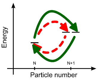
Figure 1: Interference in a single electron transistor (SET). The dynamics is governed by equivalent paths in the many-body spectrum that involve two (or more) degenerate states.

In the present paper we develop a general theory of interference blockade. We give in fact an a priori algorithm for the detection of the interference blocking states of a generic ISET. As a concrete example, we analyze the triple dot ISET (see Section IV) as it represents the simplest structure exhibiting interference blockade. In particular we concentrate on the blockade that involves an excited triplet state and we show how to prepare the system in each of the three spin states without application of any external magnetic field. Thus we obtain an interference mediated control of the electron spin in quantum dots, a highly desirable property for spintronics Wolf01 ; Awschalom07 ; Ohno00 and spin-qubit applications Golovach06 ; Levitov03 ; Debald05 ; Walls07 ; Nowak07 .

The method of choice for the study of the dynamics in those systems is the generalized master equation approach for the reduced density matrix (RDM), where coherences between degenerate states are retained Gurvitz96 ; Braun04 ; Wunsch05 ; Donarini06 ; Hornberger08 ; Darau09 ; Donarini09 ; Braig05 ; Harbola06 ; Mayrhofer07 ; Koller07 ; Pedersen07 ; Begemann08 ; Schultz09 . Such coherences give rise to precession effects and ultimately cause interference blockade.

The paper is organized as follows: in section II we introduce a generic model of ISET. In section III we set the necessary and sufficient conditions which define the interference blocking states and a generic algorithm to detect them. In section IV we apply the theory to the triple dot molecule as archetypal example of ISET. Section V closes the paper with a summary of the results and conclusive remarks.

II Generic model of ISET

Let us consider the interference single electron transistor (ISET) described by the Hamiltonian:

$$H=H_{\rm sys}+H_{\rm leads}+H_{\rm tun},$$ (1)

where $H_{\rm sys}$ represents the central system and also contains the energy shift operated by a capacitively coupled gate electrode at the potential $V_{\rm g}$. The Hamiltonian $H_{\rm sys}$ is invariant with respect to a set of point symmetry operations that defines the symmetry group of the device. This fact ensures the existence of degenerate states. In particular, for essentially planar structures belonging to the $D_{n}$ group, the (non-accidental) orbital degeneracy is at maximum twofold and can be resolved using the eigenvalues $\ell$ of the projection of the angular momentum along the principal axis of rotation. A generic eigenstate is then represented by the ket $|N\ell\sigma E\rangle$ where $N$ is the number of electrons on the system, $\sigma$ is the spin and $E$ the energy of the state. The size of the Fock space can make the exact diagonalization of $H_{\rm sys}$ a numerical challenge in its own. We will not treat here this problem and concentrate instead on the transport characteristics. $H_{\rm leads}$ describes two reservoirs of non-interacting electrons with a difference $eV_{\rm b}$ between their electrochemical potentials. Finally, $H_{\rm tun}$ accounts for the weak tunnelling coupling between the system and the leads, characteristic of SETs, and we consider the tunnelling events restricted to the atoms or to the dots closest to the corresponding lead:

$$H_{\rm tun}=t\sum_{\alpha k\sigma}(c^{\dagger}_{\alpha k\sigma}d^{\phantom{\dagger}}_{\alpha\sigma}+d^{\dagger}_{\alpha\sigma}c^{\phantom{\dagger}}_{\alpha k\sigma}),$$ (2)

where $c^{\dagger}_{\alpha k\sigma}$ creates an electron with spin $\sigma$ and momentum $k$ in lead $\alpha=L,R$, $d^{\dagger}_{\alpha\sigma}$ creates an electron in the atom or dot closest to the lead $\alpha$ and $t$ is the bare tunnelling amplitude that we assume for simplicity independent of $\alpha$, $k$ and $\sigma$.

In the weak coupling regime the dynamics essentially consists of sequential tunnelling events at the source and drain lead that induce a flow of probability between the many-body eigenstates of the system. It is natural to define, in this picture, a blocking state as a state which the system can enter but from which it can not escape. When the system occupies a blocking state the particle number can not change in time and the current vanishes. If degenerate states participate to transport, they can lead to interference since, like the two arms of an electronic interferometer, they are populated simultaneously. In particular, depending on the external parameters they can form linear superpositions which behave as blocking states. If a blocking state is the linear combination of degenerate states we call it interference blocking state.

The coupling between the system and the leads not only generates the tunneling dynamics described so far, but also contributes to an internal dynamics of the system that leaves unchanged its particle number. In fact the equation of motion for the reduced density matrix $\rho$ of the system can be cast, to lowest non vanishing order in the coupling to the leads, in the form Braun04 ; Braig05 ; Donarini09 :

$$\dot{\rho}=-\frac{i}{\hbar}[H_{\rm sys},\rho]-\frac{i}{\hbar}[H_{\rm eff},\rho]+\mathcal{L}_{\rm tun}\rho.$$ (3)

The commutator with $H_{\rm sys}$ in Eq. (3) represents the coherent evolution of the system in absence of the leads. The operator $\mathcal{L}_{\rm tun}$ describes instead the sequential tunnelling processes and is defined in terms of the transition amplitudes between the different many-body states. Finally, $H_{\rm eff}$ renormalizes the coherent dynamics associated to the system Hamiltonian and is also proportional to the system-lead tunnelling coupling. The specific form of $H_{\rm eff}$ depends on the details of the system, yet in all cases it is bias and gate voltage dependent and it vanishes for non degenerate states.

III Blocking states

III.1 Classification of the tunnelling processes

For the description of the tunnelling dynamics contained in the superoperator $\mathcal{L}_{\rm tun}$ it is convenient to classify all possible tunnelling events according to four categories: i)Creation (Annihilation) tunnelling events that increase (decrease) by one the number of electrons in the system, ii) Source (Drain) tunnelling that involves the lead with the higher (lower) chemical potential, iii) $\uparrow$ ($\downarrow$) tunnelling that involves an electron with spin up (down) with respect of the corresponding lead quantization axis, iv) Gain (Loss) tunnelling that increases (decreases) the energy in the system.

Using categories i)-iii) we can efficiently organize the matrix elements of the system component of $H_{\rm tun}$ in the matrices:

$$T^{+}_{N,EE^{\prime}}=\left(\begin{array}[]{c}t^{+}_{\rm S\uparrow}\\ t^{+}_{\rm S\downarrow}\\ t^{+}_{\rm D\uparrow}\\ t^{+}_{\rm D\downarrow}\\ \end{array}\right)\qquad T^{-}_{N,EE^{\prime}}=\left(\begin{array}[]{c}t^{-}_{\rm S\uparrow}\\ t^{-}_{\rm S\downarrow}\\ t^{-}_{\rm D\uparrow}\\ t^{-}_{\rm D\downarrow}\\ \end{array}\right)\\$$ (4)

where $S,D$ means source and drain respectively and

$$t^{+}_{\alpha\sigma}=\langle N+1,\{\ell^{\prime},\tau^{\prime}\},E^{\prime}|d^{\dagger}_{\alpha\sigma}|N,\{\ell,\tau\},E\rangle$$ (5)

is a matrix in itself, defined for every creation transition from a state with particle number $N$ and energy $E$ to one with $N+1$ particles and energy $E^{\prime}$. We indicate correspondingly in the following transitions involving $t^{+}_{S\sigma}$ and $t^{+}_{D\sigma}$ as source-creation and drain-creation transitions. The compact notation $\{\ell,\tau\}$ indicates all possible combination of the quantum numbers $\ell$ and $\tau$. It follows that the size of $t^{+}_{\alpha\sigma}$ is ${\rm mul}(N+1,E^{\prime})\times{\rm mul}(N,E)$ where the function ${\rm mul}(N,E)$ gives the degeneracy of the many-body energy level with $N$ particles and energy $E$. Analogously

$$t^{-}_{\alpha\sigma}=\langle N-1,\{\ell^{\prime},\tau^{\prime}\},E^{\prime}|d^{\phantom{\dagger}}_{\alpha\sigma}|N,\{\ell,\tau\},E\rangle$$ (6)

accounts for the annihilation transitions.

The fourth category concerns energy and it is intimately related to the first and the second. Not all transitions are in fact allowed: due to the energy conservation and the Pauli exclusion principle holding in the fermionic leads, the energy gain (loss) of the system associated to a gain (loss) transition is governed by the bias voltage. These energy conditions are summarized in the table 1 and illustrated in Fig. 2.

$\Delta E\lesssim$	Creation	Annihilation
Source	$+eV_{\rm b}/2$	$-eV_{\rm b}/2$
Drain	$-eV_{\rm b}/2$	$+eV_{\rm b}/2$

Table 1: Energy conditions for tunnelling transitions between the many-body eigenstates of the system. The quantity $\Delta E=E_{f}-E_{i}$ is the difference between the energies of the final and initial many-body states of the system involved in the transition.

The quantity $\Delta E:=E_{f}-E_{i}$, is the difference between the energy of the final and initial state of the system and the approximate condition $\lesssim$ is due to the thermal broadening of the Fermi distributions. For simplicity we set the zero of the energy at the chemical potential of the unbiased device and we assume an equal potential drop at the source and drain contact. In the table 1 one reads for example that in a source-creation tunnelling event the system can gain at maximum $\tfrac{eV_{\rm b}}{2}$ or that in a source-annihilation and drain-creation transition the system looses at least an energy of $\tfrac{eV_{\rm b}}{2}$.

From table 1 one also deduces that, from whatever initial state, it is always possible to reach the lowest energy state (the global minimum) via a series of energetically allowed transitions. Vice versa, not all states can be reached starting from the global minimum. Thus, the only relevant states for the transport in the stationary regime are the states that can be reached from the global minimum via a finite number of energetically allowed transitions.

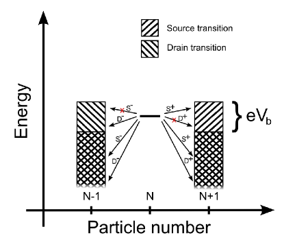
Figure 2: Energetically available transitions from an $N$ particle level. The patterned rectangles indicate the energy range of energetically available source (S) and drain (D) transitions both to states with $N+1$ and $N-1$ particles. The arrows show examples of both allowed and forbidden transitions.

III.2 Subspace of decoupled states

In the process of detecting the blocking states we observe first that some states do not participate to the transport and can be excluded a priori from any consideration. These are states with zero transition elements to all other relevant states. Within the subspace with $N$ particles and energy $E$ the decoupled states span the vector space:

$$\mathcal{D}_{N,E}=\bigcap_{E^{\prime}}\left[{\rm ker}\,\,T^{+}_{N,EE^{\prime}}\cap{\rm ker}\,\,T^{-}_{N,EE^{\prime}}\right]$$ (7)

where $E^{\prime}$ is the energy of a relevant state with $N+1$ or $N-1$ particles respectively. The function ${\rm ker}\,\,M$ returns the null space of the linear application associated to the matrix $M$.

The decoupled space $\mathcal{D}_{N,E}$ as presented in equation (7) is constructed as follows. Let us consider a generic many-body state $|\psi_{NE}\rangle$ with $N$ particles and energy $E$ and let ${\bf v}$ be the vector of its components in the basis $|N\ell\tau E\rangle$. The vector $T^{+}_{N,EE^{\prime}}\mathbf{v}$ has thus $4\times{\rm mul}(N+1,E^{\prime})$ components and consists of all possible transition amplitudes from $|\psi_{NE}\rangle$ to all possible states with $N+1$ particles and energy $E^{\prime}$. Consequently ${\rm ker}\,\,T^{+}_{N,EE^{\prime}}$ contains the vectors ${\bf v}$ associated to states with $N$ particles and energy $E$ which are decoupled from all possible states with $N+1$ particles and energy $E^{\prime}$. Analogously holds for the significance of ${\rm ker}\,\,T^{-}_{N,EE^{\prime}}$. The intersections in (7) and the condition on $E^{\prime}$ ensure that $\mathcal{D}_{N,E}$ contains only states decoupled at the same time from all other states relevant for transport in the stationary regime. We emphasize that, due to the condition on the energy $E^{\prime}$, the decoupled space $\mathcal{D}_{N,E}$ is a dynamical concept that depends on the applied gate and bias across the ISET. The coupled space $\mathcal{C}_{N,E}$ is the orthogonal complement of $\mathcal{D}_{N,E}$ in the Hilbert space with $N$ particles and energy $E$. The blocking states belong to it.

As a first simple application of the ideas presented so far, let us consider the SET at zero bias. According to the table 1 the system can only undergo loss tunnelling events and the global energy minimum is the only blocking state, in accordance with the observation that the system is in equilibrium with the leads and that we measure the energy starting from the equilibrium chemical potentialFree_energy . The potential $V_{\rm g}$ of the gate electrode defines the particle number of the global minimum and, by sweeping $V_{\rm g}$ at zero bias, one can change the number of electrons on the system one by one. This situation, the Coulomb blockade, remains unchanged until the bias is high enough to open a gain transition that unblocks the global minimum. Then, the current can flow. Depending on the gate this first unblocking transition can be of the kind source-creation or drain-annihilation. Correspondingly, the current is associated to $N\leftrightarrow N+1$ or $N\leftrightarrow N-1$ oscillations, where $N$ is the particle number of the global minimum.

III.3 Blocking conditions

At finite bias the condition which defines a blocking state becomes more elaborate:

1. The blocking state must be achievable from the global minimum with a finite number of allowed transitions.

2. All matrix elements corresponding to energetically allowed transitions outgoing from the blocking state should vanish: in particular all matrix elements corresponding to $E_{f}-E_{\rm block}<-\tfrac{eV_{b}}{2}$ and for $|E_{f}-E_{\rm block}|<\tfrac{eV_{b}}{2}$ only the ones corresponding to the drain-annihilation and source-creation transitions.

The first condition ensures the blocking state to be populated in the stationary regime. The second is a modification of the generic definition of blocking state restricted to energetically allowed transitions and it can be written in terms of the tunnelling matrices $T^{+}_{N,EE^{\prime}}$ and $T^{-}_{N,EE^{\prime}}$. For each many-body energy level $|NE\rangle$, the space spanned by the blocking states reads then:

$$\mathcal{B}_{N,E}=\mathcal{B}^{(1)}_{N,E}\cap\mathcal{B}^{(2)}_{N,E}\cap\mathcal{C}_{N,E}$$ (8)

with

$$\begin{split}\mathcal{B}^{(1)}_{N,E}=\bigcap_{E^{\prime}}&\left\{\mathcal{P}_{NE}\left[{\rm ker}\,\,(T^{+}_{N,EE^{\prime}},T_{D})\right]\cap\right.\\ &\left.\mathcal{P}_{NE}\left[{\rm ker}\,\,(T^{-}_{N,EE^{\prime}},T_{S})\right]\right\}\\ \mathcal{B}^{(2)}_{N,E}=\bigcap_{E^{\prime\prime}}&\left[{\rm ker}\,\,T^{+}_{N,EE^{\prime\prime}}\cap{\rm ker}\,\,T^{-}_{N,EE^{\prime\prime}}\right].\end{split}$$ (9)

In Eq. 9 we introduced the matrices $T_{D}=(\mathbf{0},\mathbf{1})^{T}$ and $T_{S}=(\mathbf{1},\mathbf{0})^{T}$ with $\mathbf{1}$ being the identity matrix and $\mathbf{0}$ the zero matrix, both of dimension $2\times{\rm mul}(N+1,E^{\prime})$ for $T_{D}$ and $2\times{\rm mul}(N-1,E^{\prime})$ for $T_{S}$. The energies $E^{\prime}$ and $E^{\prime\prime}$ satisfy the inequalities $|E^{\prime}-E|<\tfrac{eV_{\rm b}}{2}$ and $E^{\prime\prime}-E<-\tfrac{eV_{\rm b}}{2}$, respectively, and $\mathcal{P}_{NE}$ is the projection on the $N$ particle space with energy $E$.

The first kernel in $\mathcal{B}^{(1)}_{N,E}$ together with the projector $\mathcal{P}_{NE}$ gives all linear combinations of $N$ particle degenerate states which have a finite creation transition involving the drain but not the source lead. This condition can in fact be expressed as a non-homogeneous linear equation for the vector $\mathbf{v}$ of the components in the many body basis of the generic $N$ particle state with energy $E$:

$$T^{+}_{N,EE^{\prime}}\mathbf{v}=\mathbf{b},$$ (10)

where $\mathbf{b}$ is a generic vector of length $4\times{\rm mul}(N+1,E^{\prime})$ whose first $2\times{\rm mul}(N+1,E^{\prime})$ components (the source transition amplitudes) are set to zero. Due to the form of $\mathbf{b}$, it is convenient to transform Eq.  (10) into an homogeneous equation for a larger space of dimension ${\rm mul}(N,E)+2\times{\rm mul}(N+1,E^{\prime})$ which also contains the non-zero elements of $\mathbf{b}$ and finally project the solutions of this equation on the original space. With this procedure we can identify the space of the solutions of (10) with:

$$V=\mathcal{P}_{NE}\left[{\rm ker}\,\,(T^{+}_{N,EE^{\prime}},T_{D})\right].$$ (11)

The second kernel in $\mathcal{B}^{(1)}_{N,E}$ takes care of the annihilation transitions in a similar way. Notice that $V$ also contains vectors that are decoupled at both leads. This redundance is cured in (8) by the intersection with the coupled space $\mathcal{C}_{NE}$.

The conditions (9) are the generalization of the conditions over the tunnelling amplitudes that we gave in [Darau09, ]. That very simple condition captures the essence of the effect, but it is only valid under certain conditions: the spin channels should be independent, the relevant energy levels only two and the transition has to be between a non degenerate and a doubly degenerate level. Equation (9), on the contrary, is completely general. In appendix A we give an explicit derivation of the equivalence of the two approaches in the simple case.

For most particle numbers $N$ and energies $E$, and sufficiently high bias, $\mathcal{B}_{N,E}$ is empty. Yet, blocking states exist and the dimension of $\mathcal{B}_{N,E}$ can even be larger than one as we have already proven for the benzene and the triple dot ISETs Donarini09 . Moreover, it is most probable to find interference blocking states among ground states due to the small number of intersections appearing in (9) in this situation. Nevertheless also excited states can block the current as we will show in the next section.

The case of spin polarized leads is already included in the formalism both in the parallel and non parallel configuration. In the parallel case one quantization axis is naturally defined on the all structure and $\sigma$ in equations (5) and (6) is defined along this axis. In the case of non parallel polarized leads instead it is enough to consider $d^{\dagger}_{\alpha\sigma}$ and $d^{\phantom{\dagger}}_{\alpha\sigma}$ in equations (5) and (6), respectively, with $\sigma$ along the quantization axis of the lead $\alpha$. It is interesting to note that in that case, no blocking states can be found unless the polarization of one of the leads is $P=1$. The spin channel can in fact be closed only one at the time via linear combination of different spin states.

A last comment on the definition of the blocking conditions is necessary. A blocking state is a stationary solution of the equation (3) since by definition it does not evolve in time. The density matrix associated to one of the blocking states discussed so far i) commutes with the system Hamiltonian since it is a state with given particle number and energy; ii) it is the solution of the equation $\mathcal{L}_{\rm tun}\rho=0$ since the probability of tunnelling out from a blocking state vanishes, independent of the final state. Nevertheless, a third condition is needed to satisfy the condition of stationarity:

1. The density matrix $\rho_{\rm block}$ associated to the blocking state should commute with the effective Hamiltonian $H_{\rm eff}$ which renormalizes the coherent dynamics of the system to the lowest non vanishing order in the coupling to the leads:

   $$[\rho_{\rm block},H_{\rm eff}]=0.$$ (12)

The specific form of $H_{\rm eff}$ varies with the details of the system. Yet its generic bias and gate voltage dependence implies that, if present, the current blocking occurs only at specific values of the bias for each gate voltage. Further, if an energy level has multiple blocking states and the effective Hamiltonian distinguishes between them, selective current blocking, and correspondingly all electrical preparation of the system in one specific degenerate state, can be achieved. In particular, for spin polarized leads, the system can be prepared in a particular spin state without the application of any external magnetic field as we will show explicitly in section IV.3.

IV The triple dot ISET

The triple dot SET has been recently in the focus of intense theoreticalEmary07 ; Delgado08 ; Gong08 ; Kostyrko09 ; Shim09 ; Poeltl09 ; Busl10 and experimentalGaudreau06 ; Rogge08 ; Gaudreau09 ; Austing10 investigation due to its capability of combining incoherent transport characteristics and signatures of molecular coherence. The triple dot ISET that we consider here (Fig. 3) is the simplest structure with symmetry protected orbital degeneracy exhibiting interference blockade. Despite its relative simplicity this system displays different kinds of current blocking and it represents for this reason a suitable playground for the ideas presented so far.

IV.1 The model

We describe the system with an Hamiltonian in the extended Hubbard form:

$$\begin{split}H_{\rm sys}=\,\,&\xi_{0}\sum_{i\sigma}d^{\dagger}_{i\sigma}d^{\phantom{\dagger}}_{i\sigma}+b\sum_{i\sigma}\left(d^{\dagger}_{i\sigma}d^{\phantom{\dagger}}_{i+1\sigma}+d^{\dagger}_{i+1\sigma}d^{\phantom{\dagger}}_{i\sigma}\right)\\ +&U\sum_{i}\left(n_{i\uparrow}-\tfrac{1}{2}\right)\left(n_{i\downarrow}-\tfrac{1}{2}\right)\\ +&V\sum_{i}\left(n_{i\uparrow}+n_{i\downarrow}-1\right)\left(n_{i+1\uparrow}+n_{i+1\downarrow}-1\right),\end{split}$$ (13)

where $d^{\dagger}_{i\sigma}$ creates an electron of spin $\sigma$ in the ground state of the quantum dot $i$. Here $i=1,\ldots,\,3$ runs over the three quantum dots of the system and we impose the periodic condition $d_{4\sigma}=d_{1\sigma}$. Moreover $n_{i\sigma}=d^{\dagger}_{i\sigma}d^{\phantom{\dagger}}_{i\sigma}$. The effect of the gate is included as a renormalization of the on-site energy $\xi=\xi_{0}-eV_{\rm g}$ where $V_{\rm g}$ is the gate voltage. We measure the energies in units of the modulus of the (negative) hopping integral $b$. The parameters that we use are $\xi_{0}=0,\,U=5\,|b|,\,V=2\,|b|.$

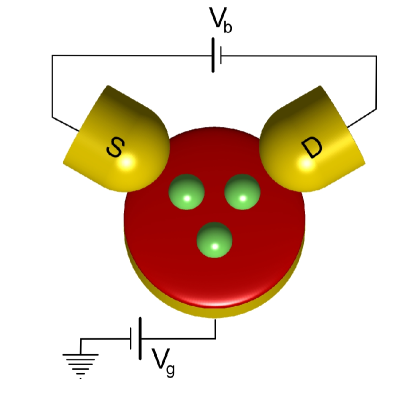
Figure 3: Schematic representation of a triple dot interference single electron transistor (ISET).

The number of electrons considered for the triple dot structure goes from 0 to 6. Thus the entire Fock space of the system contains $4^{3}=64$ states. By exact diagonalization we obtain the many body-eigenstates and the corresponding eigenvalues that we present in Fig. 4 for a gate voltage of $V_{\rm g}=4.8\,b/e$. In the table 2 we also give the degeneracies of all levels relevant for the blocking states analysis which will follow. We distinguish between spin and orbital degeneracy since the latter is the most important for the identification of the blocking states. The total degeneracy of a level is simply the product of the two.

Many-body	Orbital	Spin
energy level	degeneracy	degeneracy
$0$	1	1
$1_{0}$	1	2
$2_{0}$	1	1
$2_{1}$	2	3
$3_{0}$	2	2
$4_{0}$	1	3
$5_{0}$	2	2
$6$	1	1

Table 2: Degeneracy of the triple dot system energy levels as it follows from the underlying $D_{3}$ symmetry. A level $N_{i}$ is the $i$th excited level with $N$ particles. The total degeneracy of the level is the product of its orbital and spin degeneracies.

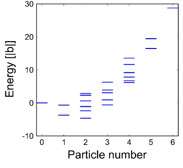
Figure 4: Spectrum of the triple dot system for the specific gate voltage $eV_{g}=4.8b$ chosen to favor a configuration with two electrons. The other parameters in the system are $U=5|b|$ and $V=2|b|$, where $b$ is the hopping integral between the different dots.

IV.2 Excited state blocking

In Fig. 5 we show the stationary current through the triple dot ISET as a function of bias and gate voltage. At low bias the current vanishes almost everywhere due to Coulomb blockade. The particle number is fixed within each Coulomb diamond by the gate voltage and the zero particle diamond is the first to the right. The zero current lines running parallel to the borders of the 6, 4 and 2 particle diamonds are instead signatures of ground state interference that involves an orbitally non-degenerate ground state (with 2, 4, and 6 particle) and an orbitally double-degenerate one (with 3 and 5 particles). In appendix A we illustrate how to obtain an expression for the blocking states in these cases.

The striking feature in Fig. 5 is the black area of current blocking sticking out of the right side of the two particles Coulomb diamond. It is the fingerprint of the occupation of an excited interference blocking state. Fig. 6 is a zoom of the current plot in the vicinity of this excited state blocking. The dashed lines indicate at which bias and gate voltage a specific transition is energetically allowed, with the notation $N_{i}$ labelling the $i$th excited many-body level with $N$ particles. These lines are physically recognizable as abrupt changes in the current and run all parallel to two fundamental directions determined by the ground state transitions. For positive bias, positive (negative) slope lines indicates the bias threshold for the opening of source-creation (drain-annihilation) transitions. The higher the bias the more transitions are open, the higher, in general, the current.

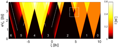
Figure 5: Stationary current for the triple dot ISET. Coulomb blockade diamonds are visible at low biases. Ground state and excited state interference blockades are also highlighted. The temperature is $k_{b}T=0.002|b|$. The other parameters are the same as the ones in Fig. 4.

The anomalous blockade region is delimited on three sides by transitions lines associated to the first excited two particle level $2_{1}$. Our group theoretical analysis shows that the two particle first excited state is a twofold orbitally degenerate spin triplet (see Table 2). In other terms we can classify its six states with the notation $|2_{1},\ell,S\rangle$ with $\ell=\pm\hbar$ being the projection of the angular momentum along the main rotation axis, perpendicular to the plane of the triple dot, and $S_{z}=-\hbar,0,\hbar$ the component of the spin along a generic quantization axis. The $1_{0}$ energy level is instead twice spin degenerate and invariant under the symmetry operations of the point group $D_{3}$.

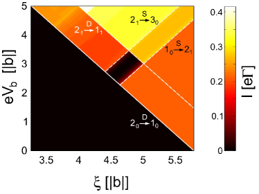
Figure 6: Blow up of the stationary current through the triple dot ISET around the 2 to 1 particle degeneracy point. The black area sticking out of the 2 particles Coulomb diamond denotes the excited states blocking.

In order to identify the 2 particle blocking states we perform the analysis presented in the previous section for the $2_{1}$ energy level with the gate and bias in the blocking region. Firstly, we find that the $2_{1}$ energy level can be reached from $2_{0}$ via the drain-annihilation transition $2_{0}\rightarrow 1_{0}$ followed by the source-creation transition $1_{0}\rightarrow 2_{1}$. Secondly, the space of the decoupled states $\mathcal{D}_{2_{1}}$ is empty and the only energetically allowed outgoing transition is the drain-annihilation $2_{1}\rightarrow 1_{0}$ transition. Thus the blocking space is given by the expression:

$$\mathcal{B}_{2_{1}}=\mathcal{P}_{2_{1}}\left[{\rm ker}\,(T^{-}_{2,2_{1}\,1_{0}},T_{S})\right]$$ (14)

and has dimension three. For clearness we give in the appendix B the explicit expression of $T^{-}_{2,2_{1}\,1_{0}}$ and the corresponding vectors that span $\mathcal{B}_{2_{1}}$. Essentially, there is a blocking state for each of the three projection of the spin $S_{z}$. This result is natural since, for unpolarized or parallel polarized leads, coherences between states of different spin projection along the common lead quantization axis do not survive in the stationary limit.

Outside the blocking region either the first or the second blocking state conditions are violated. In particular, below the lower right border the state $2_{1}$ can not be reached from the global minimum since the $1_{0}\rightarrow 2_{1}$ source-creation transition is forbidden while above the upper left (right) borders the state $2_{1}$ can be depopulated towards the $3_{0}$ ($1_{0}$) states via a source-creation (drain-annihilation) transition.

IV.3 Spin polarized transport

The orbital interference blocking presented in the previous section acquires a spin dependence in presence of polarized leads. The lead polarization $P_{\alpha}$ with $\alpha=L,R$ is defined by means of the density of states $D_{\alpha\sigma}$ at the Fermi energy for the different spin states:

$$P_{\alpha}=\frac{D_{\alpha\uparrow}-D_{\alpha\downarrow}}{D_{\alpha\uparrow}+D_{\alpha\downarrow}}$$ (15)

and is taken equal for the two leads $P=P_{L}=P_{R}$. Finally, the spin polarization influences the dynamics of the system via the spin dependent bare tunnelling rates $\Gamma^{0}_{\alpha\sigma}=\tfrac{2\pi}{\hbar}|t|^{2}D_{\alpha\sigma}$ that enter the definition of the tunnelling component of the Liouvillian $\mathcal{L}_{\rm tun}$ and the renormalization frequencies $\omega_{\alpha S_{z}}$. We assume the leads to be parallel polarized so that no spin torque is active in the device and we can exclude the spin accumulation associated to thatBraun04 ; Braig05 .

In Fig. 7 we show the current in the excited state blocking region as a function of the bias and of the (parallel) lead polarization $P$. For non-polarized leads the current is blocked at a single bias, while for finite values of $P$ the blocking is threefold. For the same bias and polarization ranges we present in Fig. 8 the $z$ component of the spin for the triple dot. The spin projection $S_{z}$ assumes, exactly in correspondence of the current blocking, the values $S_{z}=-\hbar,0,\hbar$, respectively, as the bias is increased.

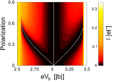
Figure 7: Current as a function of the polarization and of the bias voltage in proximity of the excited state interference blocking. The white dashed lines are defined by the conditions $\omega_{SS_{z}}=0$ for $S_{z}=-\hbar,0,\hbar$ from left to right, respectively.

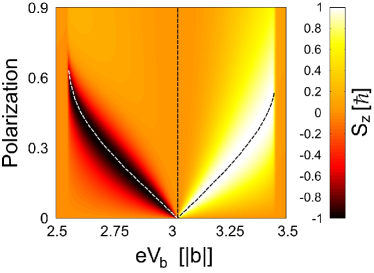
Figure 8: Spin projection $S_{z}$ as a function of the polarization and of the bias in proximity of the excited state interference blocking. Notice by comparison with Fig. 7 the correspondence between current blocking and spin preparation.

The explanation of this effect relies on the third blocking condition, Eq. (12), and concerns the form of the effective Hamiltonian introduced in Eq. (3). The latter can be written, due to the rotational symmetry of the system, in the form:

$$H_{\rm eff}=\sum_{\alpha S_{z}}\omega_{\alpha S_{z}}L_{\alpha},$$ (16)

where $L_{\alpha}$ is the projection of the angular momentum in the direction of the lead $\alpha$ and it does not depend on the spin degree of freedom $S_{z}$. Moreover, $\omega_{\alpha S_{z}}$ is the frequency renormalization given to the states of spin projection $S_{z}$ by their coupling to the $\alpha$ lead. In the appendix C we give an explicit expression for $\omega_{\alpha S_{z}}$ and $L_{\alpha}$. In Fig. 9 we plot instead $\omega_{LS_{z}}$ as a function of the bias for different polarizations. The gate is fixed at $V_{g}=4.8b/e$.

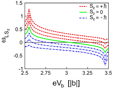
Figure 9: Renormalization frequencies as a function of the bias for different polarizations $P=0,0.25,0.5,0.75$ in the leads. The gate is $V_{g}=4.8\,b/e$. At $P=0$ all the renormalization frequencies coincide (full line). The $S_{z}=\hbar(-\hbar)$ frequency increases (decreases) monotonously with the polarization. The $S_{z}=0$ frequency is instead independent of it.

Since the two particle ground state is totally symmetric ($A_{1}$ symmetry), a three particle blocking state must be antisymmetric with respect to the vertical plane that intersects the center of the system and the drain dot. For this reason a blocking state is also an eigenstate of the projection $L_{\rm D}$ of the angular momentum in the direction of the drain lead. Consequently, the last blocking condition is satisfied only if:

$$\omega_{SS_{z}}=0$$ (17)

and the effective Hamiltonian is proportional to $L_{\rm D}$.

For zero polarization in the leads the condition (17) holds at the same bias for the three spin projections $S_{z}$ and the blocking state is a statistical mixture of the three spin projections. For polarized leads, instead, each spin projection is blocked at a specific bias and the spin on the system is controlled simply by changing the bias across the device. The dashed lines in Figs. 7 and 8 represent the solutions of equations (17) for $S_{z}=-\hbar,\,0,\,\hbar$ from left to right, respectively. Clearly they also indicate in Fig. 7 the zeros of the current and in Fig. 8 the fully populated spin states.

V Conclusions

In this paper we addressed the interference effects that characterize the transport through a symmetric single electron transistor. In particular we gave the generic conditions for interference blockade and an algorithm for the identification of the interference blocking states as linear combination of degenerate many-body eigenstates of the system.

As an application of the theory we studied the triple dot ISET. Despite its relative simplicity, this system exhibits different types of interference blocking and it represents an interesting playground of the general theory. Specifically, we concentrated on the interference blockade that involves an excited triplet state. In presence of polarized leads we exploited the interference blocking in order to access each of the triplet states by all electrical means.

The theory is sufficiently general to be applied to any device consisting of a system with degenerate many-body spectrum weakly coupled to metallic leads e.g. molecular junctions, graphene or carbon nanotube quantum dots, artificial molecules. In particular, the algebraic formulation of the blocking condition in terms of kernels of the tunnelling matrices $T^{\pm}$, Eq. (9), allows a straightforward numerical implementation and makes the algorithm directly applicable to complex junctions with highly degenerate spectrum.

VI Aknowledgments

We acknowledge financial support by the DFG under the programs SFB689, SPP1243.

Appendix A

We derive here the equation (1) in [Darau09, ] as a specific example of the general theory presented in the paper. That equation represents the interference blocking condition for the simplest possible configuration involving only a non degenerate and a doubly degenerate state.

Let us consider for simplicity a spinless Spinless system and a gate and bias condition that restricts the set of relevant many-body states to three: one with $N$ particles and two (degenerate) with $N+1$ or $N-1$ particles. The interference blocking state, if it exists, belongs to the $N\pm 1$ level. There is only one interesting tunnelling matrix to be analyzed, namely $T^{\mp}_{N\pm 1}$. Let us take for it the generic form:

$$T^{\mp}_{N\pm 1}=\left(\begin{array}[]{cc}\gamma_{S1}&\gamma_{S2}\\ \gamma_{D1}&\gamma_{D2}\\ \end{array}\right)$$ (18)

where $S$ and $D$ indicate source and drain respectively and 1 and 2 label the two degenerate states with $N\pm 1$ particles. $\gamma_{S(D)i}$ are the elements of the $t^{\mp}_{S(D)}$ matrices introduced in Eqs. (5) and (6).

The decoupled space reads:

$$\mathcal{D}_{N\pm 1}={\rm ker}\,T^{\mp}_{N\pm 1}.$$ (19)

Since the $N\pm 1$ particles relevant Hilbert space has dimension 2 the only possibility to find a blocking state is that $\mathcal{D}_{N\pm 1}=\emptyset$. In other terms:

$${\rm det}\,T^{\mp}_{N\pm 1}=\gamma_{S1}\gamma_{D2}-\gamma_{D1}\gamma_{S2}\neq 0$$ (20)

This condition is identical to Eq. (1) in Darau09 . The blocking state can finally be calculated as:

$$\begin{split}\mathcal{B}_{N+1}&=\mathcal{P}_{N+1}{\ker}\left(\begin{array}[]{ccc}\gamma_{S1}&\gamma_{S2}&1\\ \gamma_{D1}&\gamma_{D2}&0\\ \end{array}\right)\cap\mathcal{C}_{N+1}\\ \text{or}\\ \mathcal{B}_{N-1}&=\mathcal{P}_{N-1}{\ker}\left(\begin{array}[]{ccc}\gamma_{S1}&\gamma_{S2}&0\\ \gamma_{D1}&\gamma_{D2}&1\\ \end{array}\right)\cap\mathcal{C}_{N-1},\end{split}$$ (21)

where the $\mathcal{C}_{N\pm 1}$ is, in the relevant case, the entire space and the projector $\mathcal{P}_{N\pm 1}$ simply removes the last component of the vector that defines the one dimensional kernel.

Appendix B

We give here explicitly the $T^{-}_{2,2_{1}\,1_{0}}$ matrix necessary for the calculation of the triplet blocking states and the associated blocking states. The states in the $1_{0}$ doublet and in the two times orbitally degenerate triplet $2_{1}$ are labelled and ordered as follows:

$$1_{0}\,\left\{\begin{array}[]{l}|1_{0},\ell=0,\uparrow\rangle\\ |1_{0},\ell=0,\downarrow\rangle\end{array}\right.,\quad 2_{1}\,\left\{\begin{array}[]{l}|2_{1},\ell=+\hbar,S_{z}=+\hbar\rangle\\ |2_{1},\ell=+\hbar,S_{z}=0\rangle\\ |2_{1},\ell=+\hbar,S_{z}=-\hbar\rangle\\ |2_{1},\ell=-\hbar,S_{z}=+\hbar\rangle\\ |2_{1},\ell=-\hbar,S_{z}=0\rangle\\ |2_{1},\ell=-\hbar,S_{z}=-\hbar\rangle\\ \end{array}\right..$$ (22)

The elements of the $t^{-}_{\alpha\sigma}$ matrices that compose $T^{-}_{2,2_{1}\,1_{0}}$ have thus the general form:

$$t^{-}_{\alpha\sigma}(S_{z},S^{\prime}_{z},\ell)=\langle 1_{0},\ell^{\prime}=0,S_{z}^{\prime}|d^{\phantom{\dagger}}_{\alpha\sigma}|2_{1},\ell,S_{z}\rangle.$$

By orbital and spin symmetry arguments it is possible to show that

$$t^{-}_{\alpha\sigma}(S_{z},S^{\prime}_{z},\ell)=t\,e^{\frac{i}{\hbar}\ell\phi_{\alpha}}\,\delta_{S^{\prime}_{z},S_{z}-\sigma}\,(\sqrt{2}\delta_{S^{\prime}_{z},\uparrow}.+\delta_{S^{\prime}_{z},\downarrow})$$

where

$$t=\langle 1_{0},\ell^{\prime}=0,\downarrow|d^{\phantom{\dagger}}_{M\uparrow}|2_{1},\ell=1,S_{z}=0\rangle.$$

The subscript $M$ labels a reference dot and $\phi_{\alpha}$ is the angle of the rotation that brings the dot $\alpha$ on the dot $M$. The explicit form of $T^{-}_{2_{1},2_{1}\,1_{0}}$ reads:

$$T^{-}_{2,2_{1}\,1_{0}}=t\left(\begin{array}[]{cccccc}\sqrt{2}e^{-i2\pi/3}&0&0&\sqrt{2}e^{+i2\pi/3}&0&0\\ 0&e^{-i2\pi/3}&0&0&e^{+i2\pi/3}&0\\ 0&e^{-i2\pi/3}&0&0&e^{+i2\pi/3}&0\\ 0&0&\sqrt{2}e^{-i2\pi/3}&0&0&\sqrt{2}e^{+i2\pi/3}\\ \sqrt{2}e^{+i2\pi/3}&0&0&\sqrt{2}e^{-i2\pi/3}&0&0\\ 0&e^{+i2\pi/3}&0&0&e^{-i2\pi/3}&0\\ 0&e^{+i2\pi/3}&0&0&e^{-i2\pi/3}&0\\ 0&0&\sqrt{2}e^{+i2\pi/3}&0&0&\sqrt{2}e^{-i2\pi/3}\\ \end{array}\right).$$ (23)

The rank of this matrix is 6 since all columns are independent. Thus $\mathcal{C}_{2,2_{1}}$ coincides with the full Hilbert space of the first excited 2 electron energy level. The blocking space $\mathcal{B}_{2,2_{1},1_{0}}$ reads:

$$\mathcal{B}_{2,2_{1},1_{0}}=\mathcal{P}_{2_{1}}{\rm ker}(T^{-}_{2,2_{1}\,1_{0}},T_{S})$$ (24)

where $T_{S}$ reads

$$T_{S}=\left(\begin{array}[]{cccccccc}1&0&0&0&0&0&0&0\\ 0&1&0&0&0&0&0&0\\ 0&0&1&0&0&0&0&0\\ 0&0&0&1&0&0&0&0\\ \end{array}\right)^{T},$$ (25)

in accordance to its general definition given in Eq. (8), and the projector $\mathcal{P}_{2_{1}}$ removes the last four components from the vectors that span ${\rm ker}(T^{-}_{2,2_{1}\,1_{0}},T_{S})$. It is then straightforward to calculate the vectors that span the blocking space $\mathcal{B}_{2,2_{1},1_{0}}$:

$$\mathbf{v}_{1}=\left(\begin{array}[]{c}\frac{e^{-i\frac{\pi}{6}}}{\sqrt{2}}\\ 0\\ 0\\ \frac{e^{+i\frac{\pi}{6}}}{\sqrt{2}}\\ 0\\ 0\\ \end{array}\right),\quad\mathbf{v}_{2}=\left(\begin{array}[]{c}0\\ \frac{e^{-i\frac{\pi}{6}}}{\sqrt{2}}\\ 0\\ 0\\ \frac{e^{+i\frac{\pi}{6}}}{\sqrt{2}}\\ 0\\ \end{array}\right),\quad\mathbf{v}_{3}=\left(\begin{array}[]{c}0\\ 0\\ \frac{e^{-i\frac{\pi}{6}}}{\sqrt{2}}\\ 0\\ 0\\ \frac{e^{+i\frac{\pi}{6}}}{\sqrt{2}}\\ \end{array}\right).$$ (26)

The vectors $\mathbf{v}_{1},\,\mathbf{v}_{2}$ and $\mathbf{v}_{3}$ are the components of the blocking states written in the $2_{1}$ basis set presented in (22). Thus, the three blocking states correspond to the three different projectors of the total spin $S_{z}=\hbar,\,0,\,\text{and}-\hbar$, respectively.

Appendix C

We present here explicitly the renormalization frequency $\omega_{\alpha S_{z}}$ and the projection of the angular momentum $L_{\alpha}$ which appear in the expression of the effective Hamiltonian (16). The frequency $\omega_{\alpha S_{z}}$ is defined for the degenerate two particle excited level $2_{1}$ in terms of transition amplitudes to all the states of neighbor particle numbers:

$$\begin{split}\omega_{\alpha S_{z}}&=\frac{1}{\pi}\sum_{\sigma^{\prime}E}\Gamma^{0}_{\alpha\sigma^{\prime}}\\ \Big{[}&\langle 2_{1}\ell S_{z}|d^{\phantom{\dagger}}_{M\sigma^{\prime}}\,\mathcal{P}_{3E}\,d^{\dagger}_{M\sigma^{\prime}}|2_{1}\,-\!\ell\,S_{z}\rangle p_{\alpha}(E-E_{2_{1}})+\\ &\langle 2_{1}\ell S_{z}|d^{\dagger}_{M\sigma^{\prime}}\,\mathcal{P}_{1E}\,d^{\phantom{\dagger}}_{M\sigma^{\prime}}|2_{1}\,-\!\ell\,S_{z}\rangle p_{\alpha}(E_{2_{1}}\!\!-E)\Big{]},\end{split}$$ (27)

where $\mathcal{P}_{NE}\equiv\sum_{m\tau}|Nm\tau E\rangle\!\langle Nm\tau E|$ is the projector on the $N$-particle level with energy $E$ and $d^{\phantom{\dagger}}_{{\rm M}\sigma}$ destroys an electron of spin $\sigma$ in the middle dot $M$. We defined the function $p_{\alpha}(x)=-{\rm Re}\psi\left[\tfrac{1}{2}+\tfrac{i\beta}{2\pi}(x-\mu_{\alpha})\right]$, where $\beta=1/k_{\rm B}T$, $T$ is the temperature and $\psi$ is the digamma function. Moreover $\Gamma^{0}_{\alpha\sigma^{\prime}}=\tfrac{2\pi}{\hbar}|t|^{2}D_{\alpha\sigma^{\prime}}$ is the bare tunnelling rate to the lead $\alpha$ of an electron of spin $\sigma^{\prime}$, where $t$ is the tunnelling amplitude and $D_{\alpha\sigma^{\prime}}$ is the density of states for electrons of spin $\sigma^{\prime}$ in the lead $\alpha$ at the corresponding chemical potential $\mu_{\alpha}$. Due to the particular choice of the arbitrary phase of the $2$ particle excited states, $\omega_{\alpha S_{z}}$ does not depend on the orbital quantum number $\ell$. It depends instead on the bias and gate voltage through the energy of the $1$, $2_{1}$ and $3$ particle states.

In the Hilbert space generated by the two-fold orbitally degenerate $|2_{1}\,\ell\,S_{z}\rangle$ the operator $L_{\alpha}$ reads:

$$L_{\alpha}=\frac{\hbar}{2}\left(\begin{array}[]{cc}1&e^{i2\phi_{\alpha}}\\ e^{-i2\phi_{\alpha}}&1\\ \end{array}\right),$$ (28)

where $\phi_{\alpha}=\pm\tfrac{2\pi}{3}$ is the angle of which we have to rotate the triple dot system to bring the middle dot $M$ into the position of the contact dot $\alpha$. For a derivation of (28) see the supplementary material of [Donarini09, ]. For all degenerate subspaces, if no accidental degeneracy is present (like for our parameter choice), the effective Hamiltonian has the form given in (16), (27), (28), with the renormalization frequencies calculated using the appropriate energies and matrix elements.

References

- (1) T. Young, Phil. Trans. Royal Society of London 94, 12 (1804).
- (2) C. Jönsson, Z. Physik 161, 454 (1961).
- (3) P. G. Merli, G. F. Missiroli, and G. Pozzi, Am. J. Phys. 44, 306 (1976).
- (4) M. Arndt et al., Nature 401, 680 (1999).
- (5) A. Yacoby, M. Heiblum,D. Mahalu, and H. Shtrikman, Phys. Rev. Lett. 74, 4047 (1995).
- (6) S. Gustavsson, R. Leturcq, M. Studer, T. Ihn, K. and Ensslin, Nano Lett. 8, 2547 (2008).
- (7) R. Gutiérrez, F. Grossmann, and R. Schmidt, ChemPhysChem 4 1252 (2003).
- (8) D. V. Cardamone, C. A. Stafford, and S. Mazumdar, Nano Lett. 6, 2422 (2006).
- (9) S.-H. Ke, W. Yang, and U. Baranger, Nano Lett. 8, 3257 (2008).
- (10) Z. Quian, R. Li, X. Zhao, S. Hou, and S. Sanvito, Phys. Rev. B 78, 113301 (2008).
- (11) G. Begemann, D. Darau, A. Donarini, and M. Grifoni, Phys. Rev. B 77, 201406(R) (2008); 78,089901(E) (2008).
- (12) D. Darau, G. Begemann, A. Donarini, and M. Grifoni, Phys. Rev. B 79, 235404 (2009).
- (13) A. Donarini, G. Begemann, and M. Grifoni, Nano Letters 9, 2897 (2009).
- (14) C. Emary Phys. Rev. B 76 245319 (2007).
- (15) M. Busl, R. Sanchez, and G. Platero Phys.Rev. B 81 121306(R) (2010).
- (16) S. A. Wolf et al., Science 294, 1488 (2001).
- (17) D. D. Awschalom and M. E. Flatt, Nature Phys. 3 153 (2007).
- (18) H. Ohno et al., Nature 408, 944 (2000).
- (19) V. N. Golovach, M. Borhani, D. Loss, Phys. Rev. B 74, 165319 (2006).
- (20) L. Levitov, E. Rashba, Phys. Rev. B 67, 115324 (2003).
- (21) S. Debald, C. Emary, Phys. Rev. Lett. 94, 226803 (2005).
- (22) J. Walls, Phys. Rev. B 76, 195307 (2007).
- (23) K. C. Nowack, F. H. L. Koppens, Yu. V. Nazarov, L. M. K. Vandersypen, Science 318, 1430 (2007).
- (24) S. Braig and P. W. Brouwer Phys. Rev. B 71 195324 (2005).
- (25) S. A. Gurvitz and Ya. S. Prager, Phys. Rev. B 53, 15932 (1996).
- (26) M. Braun, J. König, and J. Martinek, Phys. Rev. B 70, 195345 (2004).
- (27) B. Wunsch, M. Braun, J. König, and D. Pfannkuche, Phys. Rev. B 72, 205319 (2005).
- (28) A. Donarini, M. Grifoni, and K. Richter, Phys. Rev. Lett. 97, 166801 (2006).
- (29) U. Harbola, M. Esposito, and S. Mukamel, Phys. Rev. B 74, 235309 (2006).
- (30) L. Mayrhofer and M. Grifoni, Eur. Phys. J. B 56, 107 (2007).
- (31) S. Koller, L. Mayrhofer, M. Grifoni, New J. Phys. 9, 348 (2007).
- (32) J. Pedersen, B. Lassen, A. Wacker, and M. Hettler, Phys. Rev. B 75, 235314 (2007).
- (33) R. Hornberger, S. Koller, G. Begemann, A. Donarini, and M. Grifoni Phys. Rev. B 77 245313 (2008).
- (34) M. G. Schultz, F. von Oppen Phys. Rev. B 80 033302 (2009).
- (35) If the equilibrium chemical potential is not set to zero the many-body energy spectrum should be substituted with the spectrum of the many-body free energy () where is the chemical potential of the leads at zero bias. The rest of the argumentation remains unchanged.
- (36) The assumption of a spinless system is not restrictive for parallel polarized leads and transitions between a spin singlet and a doublet since the different spin sectors decouple from each other.
- (37) F. Delgado, Y.-P. Shim, M. Korkusinski, L. Gaudreau, S. A. Studenikin, A. S. Sachrajda, and P. Hawrylak Phys. Rev. Lett. 101 226810 (2008).
- (38) W. Gong, Y. Zheng, and T. Lü Appl. Phys. Lett. 92 042104 (2008).
- (39) T. Kostyrko and B. R. Bułka Phys. Rev. B 79 075310 (2009).
- (40) Y.-P. Shim, F. Delgado, and P. Hawrylak Phys. Rev. B 80 115305 (2009).
- (41) C. Pöltl, C. Emary, and T. Brandes Phys. Rev. B 80 115313 (2009).
- (42) L. Gaudreau, S. A. Studenikin, A. S. Sachrajda, P. Zawadzki, A. Kam, J. Lapointe, M. Korkusinski, and P. Hawrylak Phys. Rev. Lett. 97 036807 (2006).
- (43) M. C. Rogge and R. J. Haug Phys. Rev. B 78 153310 (2008).
- (44) L. Gaudreau, A. S. Sachrajda, S. Studenikin, A. Kam, F. Delgado, Y. P. Shim, M. Korkusinski, and P. Hawrylak Phys. Rev. B 80 075415 (2009).
- (45) G. Austing, C. Payette, G. Yu, J. Gupta, G. Aers, S. Nair, S. Amaha and S. Tarucha Jap. Jour. of Appl. Phys. 49 04DJ03 (2010).