Non-similar collapse of singular isothermal spherical molecular cloud cores with nonzero initial velocities

Abstract

Theoretically, stars have been formed from the collapse of cores in the molecular clouds. Historically, the core had been assumed as an singular isothermal sphere (SIS), and the collapse had been investigated by a self-similar manner. This is while the rotation and magnetic field lead to non-symmetric collapse so that a spheroid shape may be occurred. Here, the resultant of the centrifugal force and magnetic field gradient is assumed to be in the normal direction of the rotational axis, and its components are supposed to be a fraction $\beta$ of the local gravitational force. In this research, a collapsing SIS core is considered to find the importance of the parameter $\beta$ for oblateness of the mass shells which are above the head of the expansion wave. We apply the Adomian decomposition method to solve the system of nonlinear partial differential equations because the collapse does not occur in a spherical symmetry with self-similar behavior. In this way, we obtain a semi-analytical relation for the mass infall rate $\dot{M}$ of the shells at the envelope. Near the rotational axis, the $\dot{M}$ decreases with increasing of the non-dimensional radius $\xi$, while a direct relation is observed between $\dot{M}$ and $\xi$ in the equatorial regions. Also, the values of $\dot{M}$ in the polar regions are greater than the equatorial values, and this difference is more often at smaller values of $\xi$. Overall, the results show that before reaching the head of expansion wave, the visible shape of the molecular cloud cores can evolve to oblate spheroids. The ratio of major to minor axes of oblate cores increases with increasing the parameter $\beta$, and its value can approach to the apparently observed elongated shapes of cores in the maps of molecular clouds such as Taurus and Perseus.

1 Introduction

Great deals are now known about dense cores in the molecular clouds that are the progenitors of protostars (e.g., di Francesco et al. 2007, Ward-Thompson et al. 2007). We know that, approximately, all cores in the maps of molecular clouds seem apparently to be elongated rather than spherical. For example, we can refer to the recent work of Curtis and Richer (2010) for two-dimensional ellipticity of cores in the Perseus molecular cloud, or to the old report of Myers et al. (1991) for apparent elongated shapes of cores in the Taurus maps. Overall, the observations show that, on average, the ratios of the major to minor axes of cores vary approximately between $1.2$ to $2$ with a mean value of $\approx 1.6$.

Determining the exact three-dimensional shape of a core from the apparent observations of the-plane-of-sky is impossible, instead statistical techniques have to be applied. Several studies have analyzed the observations in the context of a random distribution of inclinations to infer that cores are more nearly prolate than oblate (e.g., Curry 2002, Jones and Basu 2002). This prolate elongation of cores may be inferred as a remnant of their origin in filaments (e.g., Hartmann 2002). Also, models with cores forming from turbulent flows predict random triaxial shapes with a slight preference for prolateness (Gammie et al. 2003, Li et al. 2004). Although, some works indicate a preference for prolate cores, but there are many studies that consistently favour oblate shapes (e.g., Jones et al. 2001, Goodwin et al. 2002, Tassis 2007, Offner and Krumholz 2009, Tassis et al. 2009). If strong magnetic fields are present then collapsing cores are expected to be oblate (e.g., Galli and Shu 1993, Basu and Ciolek 2004, Ciolek and Basu 2006), which could also be caused by strong rotational motion (e.g., Cassen and Moosman 1981, Terebey et al. 1984).

Historically, in primary theoretical models for the collapse of cores and formation of star, an isothermal equation of state had been used, which as a consequence of subsonic communications in different parts of the cloud, an inverse square profile for density was appeared (Bodenheimer and Sweigart 1968). Larson (1969) and Penston (1969) were the first to analyze this inverse square behavior of density profile using the similarity method. In this case, which had been extended afterwards by Hunter (1977), one begin with a static cloud of constant density and follow the formation of the $r^{-2}$ density profile. In the opposite case, Shu (1977) assumed that the density is initially in inverse square profile SIS core, and constructed the expansion wave collapse solution to suggest the inside-out collapse scenario. These two limiting solutions of Hunter and Shu may be described as fast and slow collapse, respectively, and the reality may be somewhat in between (McKee and Ostriker 2007). Since then, a lot of asymptotic solutions and global numerical simulations have been found and developed in which authors have approximately considered the effects of three important mechanisms: turbulence, rotation and magnetic field (see, e.g., Hartmann 2009).

In this research, we return to the basic spherical collapse problem for polytropic spheres, which was used as idealized SIS similarity solutions by Shu (1977). In addition, we consider an initial inward flows, i.e., the conditions observed in some molecular cloud cores and used by Fatuzzo et al. (2004) to investigate its effects on the collapse of SIS. The goal of this paper is to reexamine the gravitational collapse of SIS with focus on the oblateness of a core via the effect of rotation and magnetic field. We suggest that the centrifugal force and magnetic field pressure lead to oblateness of the envelope of a molecular core before reaching the collapsing expansion wave. Since the collapse is not in a spherical symmetric manner, the similarity method can not be used. Instead, we use the Adomian decomposition method (Adomain 1994), to solve semi-analytically the system of differential equations. For this purpose, the collapse of SIS using the Adomian method is given in section 2. The non-similar collapse of SIS is investigated in section 3 in which the oblateness of the core is also obtained. Finally, the section 4 devotes to summary and conclusion.

2 Collapse of SIS by Adomian method

The initial density of a SIS is assumed to be in the form of inverse square, and the collapse is assumed to be only in the radial direction. The mass continuity equation is

$$\frac{\partial\rho}{\partial t}+\frac{1}{r^{2}}\frac{\partial}{\partial r}(r^{2}\rho u)=0,$$ (1)

where $u$ is the radial velocity which follows the force equation,

$$\frac{\partial u}{\partial t}+u\frac{\partial u}{\partial r}=-\frac{a_{s}^{2}}{\rho}\frac{\partial\rho}{\partial r}-g,$$ (2)

where $a_{s}$ is the sound speed, and the gravitational acceleration $g$ follows the Poisson’s equation,

$$\frac{1}{r^{2}}\frac{\partial}{\partial r}(r^{2}g)=4\pi G\rho.$$ (3)

Choosing the sound speed as the unit of velocity, and $[t]=1/\sqrt{4\pi G\rho_{c}}$ as the unit of time where $\rho_{c}$ is the density at the center of core, the basic equations (1)-(3) can be rewritten as follows

$$\frac{\partial\rho}{\partial t}+u\frac{\partial\rho}{\partial\xi}+\rho\frac{\partial u}{\partial\xi}+\frac{2}{\xi}\rho u=0,$$ (4)

$$\frac{\partial u}{\partial t}+u\frac{\partial u}{\partial\xi}+\frac{1}{\rho}\frac{\partial\rho}{\partial\xi}+g=0,$$ (5)

$$\frac{1}{\xi^{2}}\frac{\partial}{\partial\xi}(\xi^{2}g)=\rho,$$ (6)

where $\xi\equiv r/(a_{s}[t])$ is the nondimensional radius and the density and gravitational acceleration are non-dimensionalized by $\rho_{c}$ and $a_{s}/[t]$, respectively.

If the cloud is in hydrostatic equilibrium ($u=0$), the equations (4)-(6) lead to the Lane-Emden equation which is well-known in the theory of stellar structure (e.g., Chandrasekhar 1939). The Lane-Emden equation can be solved by the Adomian decomposition method which is found in the appendix A. The SIS is a special case of the Lane-Emden equation with inverse square density which do not conform the boundary conditions. Here, we choose the initial density as $\rho(\xi,0)=\Lambda/\xi^{2}$ where $\Lambda$ is the overdensity parameter with $\Lambda=2$ for hydrostatic equilibrium. The boundary condition for gravitational acceleration is $g(0,t)=0$, and we assume that the initial velocity is inward so that $u(\xi,0)=-u_{\infty}$ where $u_{\infty}$ is constant.

As mentioned in the appendix A, for using the Adomian decomposition method, equations (4)-(6) must be rewritten as

$$L_{t}\rho+N_{1}(\rho,u)=0,$$ (7)

$$L_{t}u+g+N_{2}(\rho,u)=0,$$ (8)

$$L_{\xi\xi}g-\rho=0,$$ (9)

where $L_{t}(\circ)\equiv\frac{d(\circ)}{dt}$ and $L_{\xi\xi}(\circ)\equiv\frac{1}{\xi^{2}}\frac{d}{d\xi}\left(\xi^{2}\frac{d(\circ)}{d\xi}\right)$ are operators, and

$$N_{1}(\rho,u)\equiv u\frac{\partial\rho}{\partial\xi}+\rho\frac{\partial u}{\partial\xi}+\frac{2}{\xi}\rho u,$$ (10)

$$N_{2}(\rho,u)\equiv u\frac{\partial u}{\partial\xi}+\frac{1}{\rho}\frac{\partial\rho}{\partial\xi},$$ (11)

are the nonlinear terms of the differential equations which can be written by Adomian series $N_{j}(\rho,u)=\sum_{n=0}^{\infty}A_{n}^{(j)}$ for $j=1,2$ where

$$A_{n}^{(j)}=\frac{1}{n!}\lim_{\lambda\rightarrow 0}\left[\frac{\partial^{n}}{\partial\lambda^{n}}N_{j}\left(\sum_{i=0}^{n}\rho_{i}\lambda^{i},\sum_{i=0}^{n}u_{i}\lambda^{i}\right)\right],$$ (12)

are the Adomian polynomials (Adomian 1994). In this way, the final solutions are given by the series $\rho=\sum_{n=0}^{\infty}\rho_{n}$, $u=\sum_{n=0}^{\infty}u_{n}$ and $g=\sum_{n=0}^{\infty}g_{n}$ which the terms can be obtained by the recurrence relations

$$\rho_{n+1}=-L_{t}^{-1}A_{n}^{(1)},$$ (13)

$$u_{n+1}=-L_{t}^{-1}(g_{n}+A_{n}^{(2)}),$$ (14)

$$g_{n+1}=L_{\xi\xi}^{-1}\rho_{n},$$ (15)

where $L_{t}^{-1}(\circ)\equiv\int(\circ)dt$ and $L_{\xi\xi}^{-1}(\circ)\equiv\int\xi^{-2}\left(\int\xi^{2}(\circ)d\xi\right)d\xi$ are the integration operators and the $n=0$ terms are from initial and boundary conditions: $\rho_{0}\equiv\rho(\xi,0)$, $u_{0}\equiv u(\xi,0)$ and $g_{0}\equiv g(0,t)$.

Using the mathematical softwares such as Maple (see, appendix B), the density and inward velocity are obtained as follows

$$\rho=\frac{\Lambda}{\xi^{2}}\left[1-\frac{(\Lambda-2)}{2}\frac{t^{2}}{\xi^{2}}+u_{\infty}\frac{2(\Lambda-2)}{3}\frac{t^{3}}{\xi^{3}}+\frac{(\Lambda-2)(6-2\Lambda+3u_{\infty}^{2})}{4}\frac{t^{4}}{\xi^{4}}+O\left(\frac{t^{5}}{\xi^{5}}\right)\right]$$ (16)

$$u=-u_{\infty}-(\Lambda-2)\frac{t}{\xi}\left[1-\frac{u_{\infty}}{2}\frac{t}{\xi}+\frac{(6-\Lambda+2u_{\infty}^{2})}{6}\frac{t^{2}}{\xi^{2}}-\frac{(24-5\Lambda+3u_{\infty}^{2})u_{\infty}}{12}\frac{t^{3}}{\xi^{3}}\right]+O\left(\frac{t^{5}}{\xi^{5}}\right),$$ (17)

respectively. In the case of $u_{\infty}=0$, these results reduce to the equation (19) of the well-known paper of Shu (1977) in which the similarity variable $x$ is replaced by $t/\xi$ (note that equations (45) and (46) of Fatuzzo et al. 2004 are mistyped). According to the convergence problem in the series of Adomian decomposition method (as mentioned in appendix A), the results (16) and (17) are reliable in the range of $t/\xi<1$. Thus, the solutions (16) and (17) are acceptable only for the outer regions from the head of the expansion wave (i.e., $\xi=t$), and the mass infall rate $\dot{M}\equiv 4\pi\xi^{2}\rho\mid u\mid$ of the shells in the envelope can be determined. For the inner regions of expansion wave, the terms of series (16) and (17) are not convergent, thus, we must use the suitable methods such as piecewise-adaptive decomposition method (e.g., Ramos 2009) which is beyond the scope of this research.

3 Non-similar collapse of SIS

The cores of molecular clouds rotate and the magnetic fields are also the non-eliminating parts of this medium. In this section, we investigate the effect of these mechanisms on the dynamics of collapsing SIS core. In this case, the infall velocity of matter in the spherical coordinate have two components as $\mathbf{v}=\hat{r}u+\hat{\theta}w$ so that the mass continuity equation is expressed as

$$\frac{\partial\rho}{\partial t}+\frac{1}{\xi^{2}}\frac{\partial}{\partial\xi}(\xi^{2}\rho u)+\frac{1}{\xi\sin\theta}\frac{\partial}{\partial\theta}(\sin\theta\rho w)=0,$$ (18)

which is non-dimensionalized according to the units given in section 2. Here, the effect of the centrifugal force and pressure of magnetic field, in the envelope of the core, are assumed to be in the normal direction of the rotational axis as follows

$$\mathbf{F}_{mag+rot}=\hat{r}F_{\xi}\sin^{2}\theta+\hat{\theta}F_{\theta}\sin 2\theta,$$ (19)

where for simplicity, the components are assumed to be a fraction of the local gravitational force as $F_{\xi}=-\beta\partial\phi/\partial\xi$ and $F_{\theta}=-\beta\partial\phi/\partial\theta$ where the magnetic-rotational parameter $0\leq\beta\leq 1$ indicates the importance of rotation and magnetic field, and $\phi$ is the gravitational potential which follows the Poisson’s equation,

$$\frac{1}{\xi^{2}}\frac{\partial}{\partial\xi}(\xi^{2}\frac{\partial\phi}{\partial\xi})+\frac{1}{\xi^{2}\sin\theta}\frac{\partial}{\partial\theta}(\sin\theta\frac{\partial\phi}{\partial\theta})=\rho.$$ (20)

In this way, the force equation have two components as follows

$$\frac{\partial u}{\partial t}+u\frac{\partial u}{\partial\xi}+\frac{w}{\xi}\frac{\partial u}{\partial\theta}=-\frac{1}{\rho}\frac{\partial\rho}{\partial\xi}-(1-\beta\sin^{2}\theta)\frac{\partial\phi}{\partial\xi},$$ (21)

$$\frac{\partial w}{\partial t}+u\frac{\partial w}{\partial\xi}+\frac{w}{\xi}\frac{\partial w}{\partial\theta}=-\frac{1}{\rho\xi}\frac{\partial\rho}{\partial\theta}-(1-\beta\sin 2\theta)\frac{1}{\xi}\frac{\partial\phi}{\partial\theta}.$$ (22)

Since the components of gravitational force, $\partial\phi/\partial\xi$ and $\partial\phi/\partial\theta$, are zero at the center of the core, the boundary condition of the gravitational potential at $\xi=0$ is assumed to be $\phi(0,t)=0$. At the beginning of collapse, the components of velocity are assumed to be $u(r,0)=-u_{\infty}$ and $w(r,0)=0$, and the initial density is assumed as the density of SIS: $\rho(\xi,0)=\Lambda/\xi^{2}$. We rewrite the the equations (18), (20), (21) and (22) in the Adomian form as follows

$$L_{t}\rho+N_{1}(\rho,u,w)=0,$$ (23)

$$L_{\xi\xi}\phi+\frac{1}{\xi^{2}}\frac{\partial^{2}\phi}{\partial\theta^{2}}+\frac{\cot\theta}{\xi^{2}}\frac{\partial\phi}{\partial\theta}-\rho=0,$$ (24)

$$L_{t}u+(1-\beta\sin^{2}\theta)\frac{\partial\phi}{\partial\xi}+N_{2}(\rho,u,w)=0,$$ (25)

$$L_{t}w+(1-\beta\sin 2\theta)\frac{1}{\xi}\frac{\partial\phi}{\partial\theta}+N_{3}(\rho,u,w)=0,$$ (26)

respectively, where the nonlinear terms are

$$N_{1}(\rho,u,w)\equiv u\frac{\partial\rho}{\partial\xi}+\rho\frac{\partial u}{\partial\xi}+\frac{2}{\xi}\rho u+\frac{w}{\xi}\frac{\partial\rho}{\partial\theta}+\frac{\rho}{\xi}\frac{\partial w}{\partial\theta}+\frac{\cot\theta}{\xi}\rho w,$$ (27)

$$N_{2}(\rho,u,w)\equiv u\frac{\partial u}{\partial\xi}+\frac{w}{\xi}\frac{\partial u}{\partial\theta}+\frac{1}{\rho}\frac{\partial\rho}{\partial\xi},$$ (28)

$$N_{3}(\rho,u,w)\equiv u\frac{\partial w}{\partial\xi}+\frac{w}{\xi}\frac{\partial w}{\partial\theta}+\frac{1}{\rho\xi}\frac{\partial\rho}{\partial\theta}.$$ (29)

In this way, by appointment the Adomian polynomials,

$$A_{n}^{(j)}=\frac{1}{n!}\lim_{\lambda\rightarrow 0}\left[\frac{\partial^{n}}{\partial\lambda^{n}}N_{j}\left(\sum_{i=0}^{n}\rho_{i}\lambda^{i},\sum_{i=0}^{n}u_{i}\lambda^{i},\sum_{i=0}^{n}w_{i}\lambda^{i}\right)\right],$$ (30)

for $j=1,2,3$, we receive to the recurrence relations as follows

$$\rho_{n+1}=-L_{t}^{-1}A_{n}^{(1)},$$ (31)

$$\phi_{n+1}=-L_{\xi\xi}^{-1}\left[\frac{1}{\xi^{2}}\frac{\partial^{2}\phi_{n}}{\partial\theta^{2}}+\frac{\cot\theta}{\xi^{2}}\frac{\partial\phi_{n}}{\partial\theta}-\rho_{n}\right],$$ (32)

$$u_{n+1}=-L_{t}^{-1}\left[(1-\beta\sin^{2}\theta)\frac{\partial\phi_{n}}{\partial\xi}+A_{n}^{(2)}\right],$$ (33)

$$w_{n+1}=-L_{t}^{-1}\left[(1-\beta\sin 2\theta)\frac{1}{\xi}\frac{\partial\phi_{n}}{\partial\theta}+A_{n}^{(3)}\right],$$ (34)

where the $n=0$ terms are given by the initial and boundary conditions. Thus, we can obtain the terms of the series $\rho=\sum_{n=0}^{\infty}\rho_{n}$, $u=\sum_{n=0}^{\infty}u_{n}$, $w=\sum_{n=0}^{\infty}w_{n}$ and $\phi=\sum_{n=0}^{\infty}\phi_{n}$ with a mathematical software such as Maple (see, appendix B). Here, we turn our attention to the mass infall rate, $\dot{M}\equiv 4\pi\xi^{2}\rho\mid u\mid$, at the envelope of the core ($\xi>t$) where the Adomian decomposition method is reliable. The result is

$$\dot{M}=4\pi\Lambda u_{\infty}+4\pi\Lambda(\Lambda-2-\Lambda\beta\sin^{2}\theta)\frac{t}{\xi}-4\pi\Lambda(\Lambda-2-\Lambda\beta\sin^{2}\theta)u_{\infty}\frac{t^{2}}{\xi^{2}}+O\left(\frac{t^{3}}{\xi^{3}}\right),$$ (35)

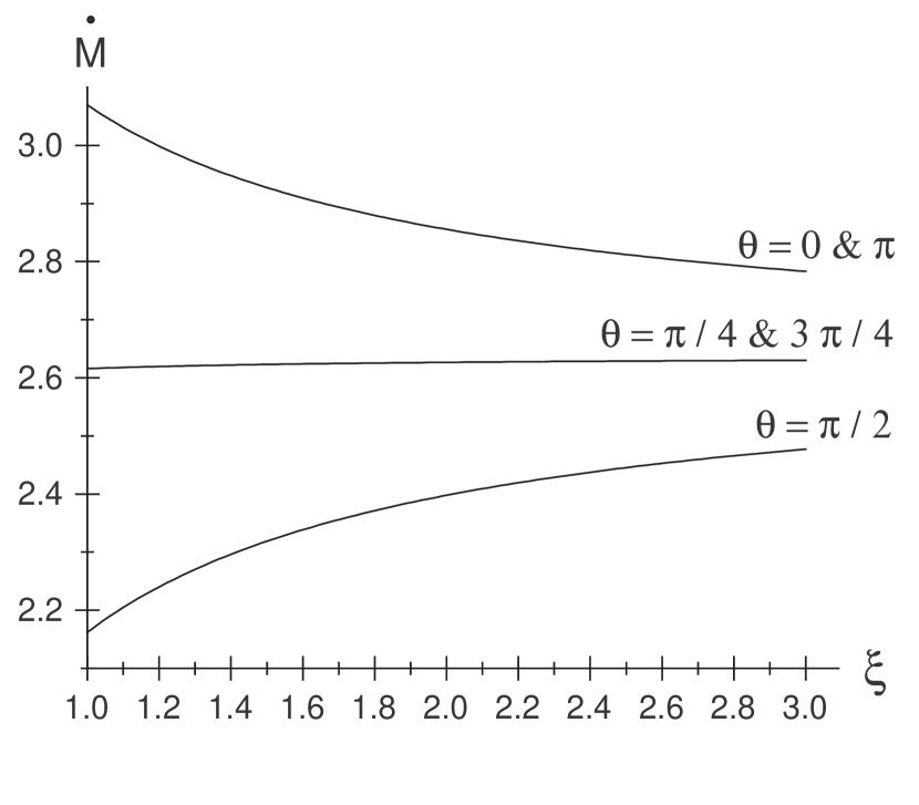
(a)

(b)

Figure 1: Mass infall rate versus (a) nondimensional length $\xi$, and (b) polar angle $\theta$, with $\Lambda=2.1$, $u_{\infty}=0.1$ and $\beta=0.1$, at time $t=1/6$.

which its values for $\Lambda=2.1$, $u_{\infty}=0.1$ and $\beta=0.1$, at time $t=1/6$ are shown in Fig.1.

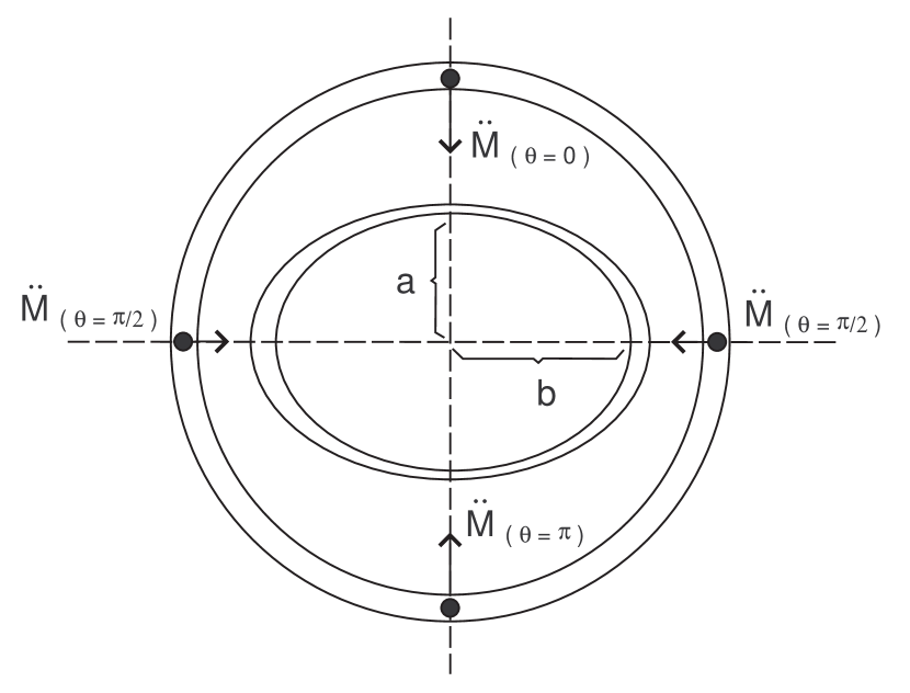
Figure 2: Schematic diagram for mass infall rate which leads to the formation of a spheroidal shell from an initial spherical shell.

Since the infall rates at the polar and equatorial regions are different, an initial spherical shell at the outer region of expansion wave, will be spheroid by time, as schematically shown in Fig. 2. In the first order approximation of mass infall rate (i.e., in the order of $t/\xi$), ratio of major to minor axes of the spheroid can be approximated as

$$\frac{b}{a}\equiv\frac{\xi-u_{\infty}t-\frac{1}{2}\ddot{M}_{(\theta=\pi/2)}t^{2}}{\xi-u_{\infty}t-\frac{1}{2}\ddot{M}_{(\theta=0)}t^{2}}.$$ (36)

Inserting $\ddot{M}\simeq 4\pi\Lambda(\Lambda-2-\Lambda\beta\sin^{2}\theta)/\xi$, which is obtained from equation (35), we have

$$\frac{b}{a}=\frac{1-u_{\infty}\frac{t}{\xi}-2\pi\Lambda(\Lambda-2-\Lambda\beta)\frac{t^{2}}{\xi^{2}}}{1-u_{\infty}\frac{t}{\xi}-2\pi\Lambda(\Lambda-2)\frac{t^{2}}{\xi^{2}}},$$ (37)

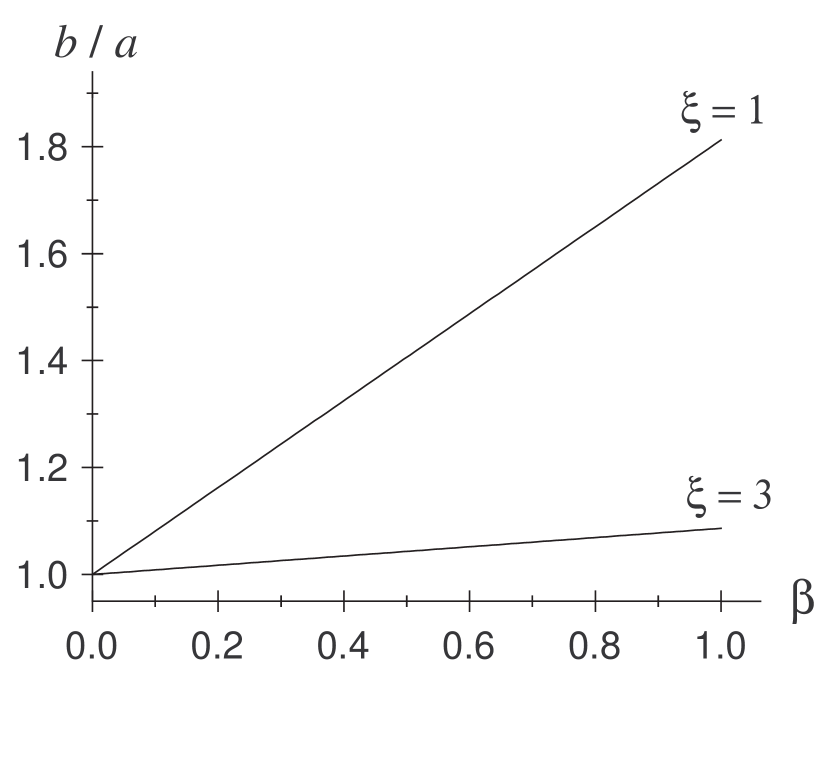
(a)

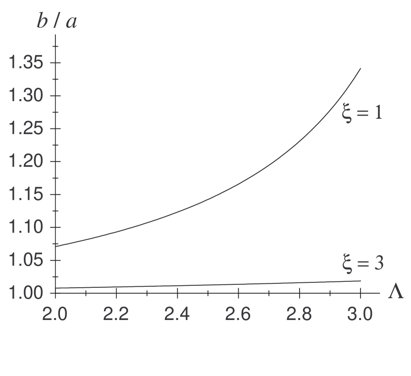
(b)

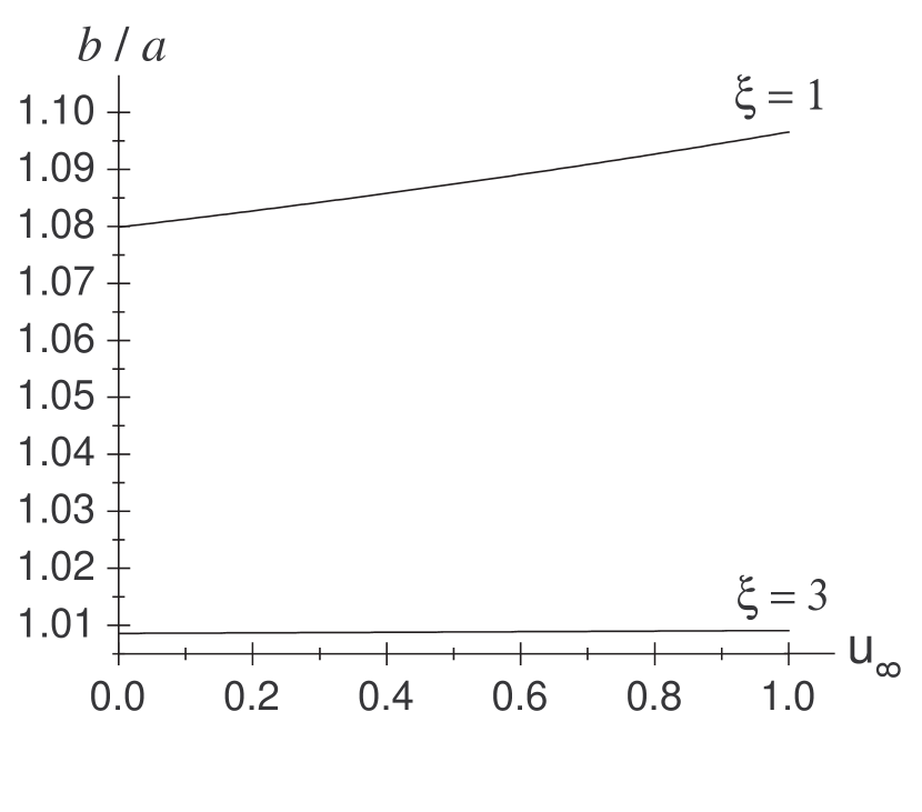
(c)

Figure 3: The ratio of major to minor axes of spheroidal shells of a core, at time $t=1/6$, versus (a) magnetic-rotational parameter $\beta$ with $\Lambda=2.1$ and $u_{\infty}=0.1$, (b) overdensity parameter $\Lambda$ with $\beta=0.1$ and $u_{\infty}=0.1$, and (c) inward initial velocity $u_{\infty}$ with $\Lambda=2.1$ and $\beta=0.1$.

which is depicted in Fig. 3 at time $t=1/6$.

4 Summary and conclusions

Stars have been formed from collapse of cores in the molecular clouds. A basic standard model for collapse of cores assumes a SIS, in which the collapse occurs inside-out accompanied with an expansion wave. We know that not only the molecular cores rotate, but also the magnetic fields affect on their dynamics. If we assume that the effect of centrifugal force and magnetic pressure are in the normal direction of the rotational axis, we expect that the shape of the envelope of core (outer regions from the head of expansion wave) be modified to a spheroid. In this case which the collapse is in a non-symmetric manner, we used the Adomian decomposition method to solve the differential equations. In the appendix A, we solved the well-known Lane-Emden equation to find that the Adomian method is applicable. Then, in section 2, the collapse of a SIS core is investigated. The results show that the Adomian decomposition method presents convergent solutions only for the regions outer than the head of the expansion wave (i.e., envelope).

In section 3, non-similar collapse of a SIS core, which is affected by the centrifugal force and magnetic pressure, is solved by the Adomian decomposition method. The mass infall rate of the shells in the envelope of the core is obtained and depicted in Fig.1 with typical values of the parameters. According to Fig. 1(a), the mass infall rate in the polar regions (near the rotational axis) decreases with increasing of radius, while in equatorial regions, the mass infall rate in the regions far from the head of expansion wave is greater than regions near to it. Fig. 1(b) shows that the mass infall rate in equatorial regions are less than polar regions, thus, before reaching the expansion wave, shape of the envelope converts to a spheroid as shown schematically in the Fig. 2.

In this way, according to mass infall rate, we determined the ratio of major to minor axes of the spheroid, and its values are shown in the Fig. 3 with typical values of the parameters. We see that the ratio of major to minor axes of spheroid do not strongly depend on the initial inward velocity $u_{\infty}$, while its value depends on the overdensity parameter $\Lambda$ and magnetic-rotational parameter $\beta$. Thus, the results show that the magnetic field and rotation lead to non-symmetric collapse so that before reaching the head of expansion wave, the apparent shape of the envelope will be converted to the triaxial oblate spheroids. Also, the results show that the ratio of major to minor axes of the spheroids can reach to the values which are consistent with the observed maps of the cores in the molecular clouds such as Taurus and Perseus.

Appendix A Solving the Lane-Emden equation by Adomian decomposition method

A spherical polytropic gas, in hydrostatic equilibrium, satisfies the equation

$$\frac{1}{\rho}\frac{dp}{dr}=-\frac{GM(r)}{r^{2}},$$ (A1)

where $M(r)$ is the mass inside the radius $r$ and the polytropic pressure is $p=\kappa\rho^{\Gamma}$, which in the isothermal case, we have $\kappa=a_{s}^{2}$ and $\Gamma=1$, where $a_{s}$ is the isothermal sound speed. Substituting $\rho=\rho_{c}\exp(-\psi)$ into equation (A1), we have

$$\frac{1}{\xi^{2}}\frac{\partial}{\partial\xi}\left[\xi^{2}e^{(1-\Gamma)\psi}\frac{d\psi}{d\xi}\right]=e^{-\psi},$$ (A2)

where $\xi\equiv\left(\frac{4\pi G}{\kappa\Gamma\rho_{c}^{\Gamma-2}}\right)^{1/2}$ is the nondimensional radius. In the isothermal case, the equation (A2) reduces to the well-known Lane-Emden equation. The boundary conditions are $\psi_{(\xi=0)}=0$ and $\left(d\psi/d\xi\right)_{\xi=0}=0$. Thus, the equation (A2) can straightforwardly be solved by numerical methods such as fourth-order Runge-Kutta.

Here, we solve the equation (A2) by the Adomian decomposition method, then we compare the result with the numerical method. For this purpose, we rewrite the equation (A2) as follows

$$L_{\xi\xi}\psi+N(\psi)=0,$$ (A3)

where $L_{\xi\xi}(\circ)\equiv\frac{1}{\xi^{2}}\frac{d}{d\xi}\left(\xi^{2}\frac{d(\circ)}{d\xi}\right)$ is the operator, and nonlinear terms of the differential equation are assembled in the function $N(\psi)\equiv(1-\Gamma)\left(\frac{d\psi}{d\xi}\right)^{2}-e^{(\Gamma-2)\psi}$. The basis of the Adomian decomposition method is to replace the function $\psi$ by a series $\psi=\sum_{n=0}^{\infty}\psi_{n}$, and the nonlinear term $N(\psi)$ by a Taylor expansion series $N(\psi)=\sum_{n=0}^{\infty}A_{n}$ where $A_{n}$ are Adomian polynomials

$$A_{0}=N(\psi_{0}),$$

$$A_{1}=\psi_{1}\left(\frac{d\psi}{d\xi}\right)_{\psi=\psi_{0}},$$

$$A_{2}=\psi_{2}\left(\frac{d\psi}{d\xi}\right)_{\psi=\psi_{0}}+\frac{1}{2!}\psi_{1}^{2}\left(\frac{d^{2}\psi}{d\xi^{2}}\right)_{\psi=\psi_{0}},$$ (A4)

and so on (Adomian 1994), which can be expressed in the general form

$$A_{n}=\frac{1}{n!}\lim_{\lambda\rightarrow 0}\left[\frac{d^{n}}{d\lambda^{n}}N\left(\sum_{i=0}^{n}\psi_{i}\lambda^{i}\right)\right],$$ (A5)

where $\lambda$ is only a dummy variable which is inserted to recover the equations (A).

In this way, the equation (A2) leads to a recurrence relation

$$\psi_{n+1}=-L_{\xi\xi}^{-1}A_{n},$$ (A6)

where $L_{\xi\xi}^{-1}(\circ)\equiv\int\xi^{-2}\left(\int\xi^{2}(\circ)d\xi\right)d\xi$ is the integration operator and $\psi_{0}\equiv\psi_{(\xi=0)}$. Thus, we can determine the $\psi_{n}$s with help of any mathematical softwares such as Maple (see, appendix B). The result is a series as

$$\psi=a_{2}\xi^{2}+a_{4}\xi^{4}+a_{6}\xi^{6}+...,$$ (A7)

where the coefficient are

$$a_{2}=+\frac{1}{3!},$$

$$a_{4}=-\frac{1}{3}(8-5\Gamma)\frac{1}{5!},$$

$$a_{6}=+\frac{2}{3}\left[4(2-\Gamma)^{2}+5(2-\Gamma)(1-\Gamma)+\frac{8}{3}(1-\Gamma)^{2}\right]\frac{1}{7!},$$ (A8)

and so on. In isothermal case ($\Gamma=1$), this result reduces to the result of Wazwaz (2001). In Fig. 4, the ratio of density to central density, $\frac{\rho}{\rho_{c}}=e^{-\psi}$, in the isothermal case, which is obtained from three terms of the series (A) is compared to the numerical results, which are obtained from the fourth-order Runge-Kutta method. As can be seen, the Adomian decomposition method gives reliable solutions for $\xi<2$. This is because of using the Taylor expansion which destroys the convergence of the series at large $\xi$ (Liao 2003, Singh et al. 2009). Substituting the appropriate values of the typical molecular clouds, we have

$$\xi=\frac{r_{(\mathrm{pc})}}{0.03\mathrm{pc}\left(\frac{T}{10\mathrm{K}}\right)^{1/2}\left(\frac{n_{c}}{10^{4}\mathrm{cm^{-3}}}\right)^{-1/2}},$$ (A9)

where $n_{c}$ is the number density at the center of the core. Thus, in the hydrostatic equilibrium of a typical molecular cloud core, the results which are obtained by the Adomian decomposition method, are usable only for radii less than $\sim 0.06\mathrm{pc}$.

Appendix B Maple programs

• The Maple program for the Lane-Emden equation is as follows:
  > psi[0]:= 0:
> n:= 0:
> N:= proc (psi) options operator, arrow;
(1-Gamma)*(diff(psi,xi))^2-exp((Gamma-2)*psi)
end proc:
> psi[1]:= -int(xi^(-2)*int( xi^2*N(psi[0]),xi),xi):
> for n from 1 to 7 do
N:= proc (psi) options operator, arrow;
(1-Gamma)*(diff(psi,xi))^2-exp((Gamma-2)*psi)
end proc:
psisum:= sum(psi[m]*lambda[n]^m,m=0..n):
A[n]:= (diff(N(psisum),$(lambda[n],n)))/factorial(n):
lambda[n]:= 0:
psi[n+1]:= -int(xi^(-2)*int(xi^2*A[n],xi),xi):
end do:
> psitotal:= collect(sum(psi[m],m=0..n),xi);
  

• The Maple program for the collapse of SIS is as follows:
  > g[0]:= 0:
> rho[0]:= Lambda/xi^2:
> u[0]:= -u[infinity]:
> n:= 0:
> N1:= proc (rho,u) options operator, arrow;
u*diff(rho,xi)+rho*diff(u,xi)+2*u*rho/xi
end proc:
> N2:= proc (rho,u) options operator, arrow;
u*diff(u,xi)+rho^(-1)*diff(rho,xi)
end proc:
> g[1]:= xi^(-2)*int(xi^2*rho[0],xi):
> rho[1]:= -int(N1(rho[0],u[0]),t):
> u[1]:= -int(g[0]+N2(rho[0],u[0]),t):
> for n from 1 to 7 do
N1:= proc (rho,u) options operator, arrow;
u*diff(rho,xi)+rho*diff(u,xi)+2*u*rho/xi
end proc:
N2:= proc (rho,u) options operator, arrow;
u*diff(u,xi)+rho^(-1)*diff(rho,xi)
end proc:
rhosum:= sum(rho[m]*lambda[n]^m,m=0..n):
usum:= sum(u[m]*lambda[n]^m,m=0..n):
A1[n]:= (diff(N1(rhosum,usum),$(lambda[n],n)))/factorial(n):
A2[n]:= (diff(N2(rhosum,usum),$(lambda[n],n)))/factorial(n):
lambda[n]:= 0:
g[n+1]:= xi^(-2)*int(xi^2*rho[n],xi):
rho[n+1]:= -int(A1[n],t):
u[n+1]:= -int(g[n]+A2[n],t):
end do:
> rhototal:= collect(sum(rho[m],m=0..n),t);
> utotal:= collect(sum(u[m],m=0..n),t);
> gtotal:= collect(sum(g[m],m=0..n),t);
  

• The Maple program for the non-similar collapse of SIS is as follows:
  > Phi[0]:= 0:
> rho[0]:= Lambda/xi^2:
> u[0]:= -u[infinity]:
> w[0]:= 0:
> n:= 0:
> N1:= proc (rho,u,w) options operator, arrow;
u*diff(rho,xi)+rho*diff(u,xi)+2*u*rho/xi+rho/xi*diff(w,theta)
+w/xi*diff(rho,theta)+cot(theta)*rho*w/xi
end proc:
> N2:= proc (rho,u,w) options operator, arrow;
u*diff(u,xi)+w/xi*diff(u,theta)+rho^(-1)*diff(rho,xi)
end proc:
> N3:= proc (rho,u,w) options operator, arrow;
u*diff(w,xi)+w/xi*diff(w,theta)+rho^(-1)*diff(rho,theta)/xi
end proc:
> Phi[1]:= -int(xi^(-2)*int(xi^2*(diff(Phi[0],theta,theta)/xi^2
+cot(theta)*diff(Phi[0],theta)/xi^2-rho[0]),xi),xi):
> rho[1]:= -int(N1(rho[0],u[0],w[0]),t):
> u[1]:= -int((1-beta*(sin(theta))^2)*diff(Phi[0],xi)
+N2(rho[0],u[0],w[0]),t):
> w[1]:= -int((1-beta*sin(2*theta))*diff(Phi[0],theta)/xi
+N3(rho[0],u[0],w[0]),t):
> for n from 1 to 7 do
N1:= proc (rho,u,w) options operator, arrow;
u*diff(rho,xi)+rho*diff(u,xi)+2*u*rho/xi+rho/xi*diff(w,theta)
+w/xi*diff(rho,theta)+cot(theta)*rho*w/xi
end proc:
N2:= proc (rho,u,w) options operator, arrow;
u*diff(u,xi)+w/xi*diff(u,theta)+rho^(-1)*diff(rho,xi)
end proc:
N3:= proc (rho,u,w) options operator, arrow;
u*diff(w,xi)+w/xi*diff(w,theta)+rho^(-1)*diff(rho,theta)/xi
end proc:
rhosum:=sum(rho[m]*lambda[n]^m,m=0..n):
usum:=sum(u[m]*lambda[n]^m,m=0..n):
wsum:=sum(w[m]*lambda[n]^m,m=0..n):
A1[n]:= (diff(N1(rhosum,usum,wsum),$(lambda[n],n)))/factorial(n):
A2[n]:= (diff(N2(rhosum,usum,wsum),$(lambda[n],n)))/factorial(n):
A3[n]:= (diff(N3(rhosum,usum,wsum),$(lambda[n],n)))/factorial(n):
A4[n]:= (diff(N4(rhosum,usum,wsum),$(lambda[n],n)))/factorial(n):
lambda[n]:=0:
Phi[n+1]:=-int(xi^(-2)*int(xi^2*(diff(Phi[n],theta,theta)/xi^2
+cot(theta)*diff(Phi[n],theta)/xi^2-rho[n]),xi),xi):
rho[n+1]:=-int(A1[n],t):
u[n+1]:=-int((1-beta*(sin(theta))^2)*diff(Phi[n],xi)+A2[n],t):
w[n+1]:=-int((1-beta*sin(2*theta))*diff(Phi[n],theta)/xi+A3[n],t):
end do:
> rhototal:=collect(sum(rho[m],m=0..n),t):
> utotal:=collect(sum(u[m],m=0..n),t):
> wtotal:=collect(sum(w[m],m=0..n),t):
> phitotal:=collect(sum(Phi[m],m=0..n),t):
> mdot:=collect(4*Pi*xi^2*(rhototal)*(-utotal),t);
  

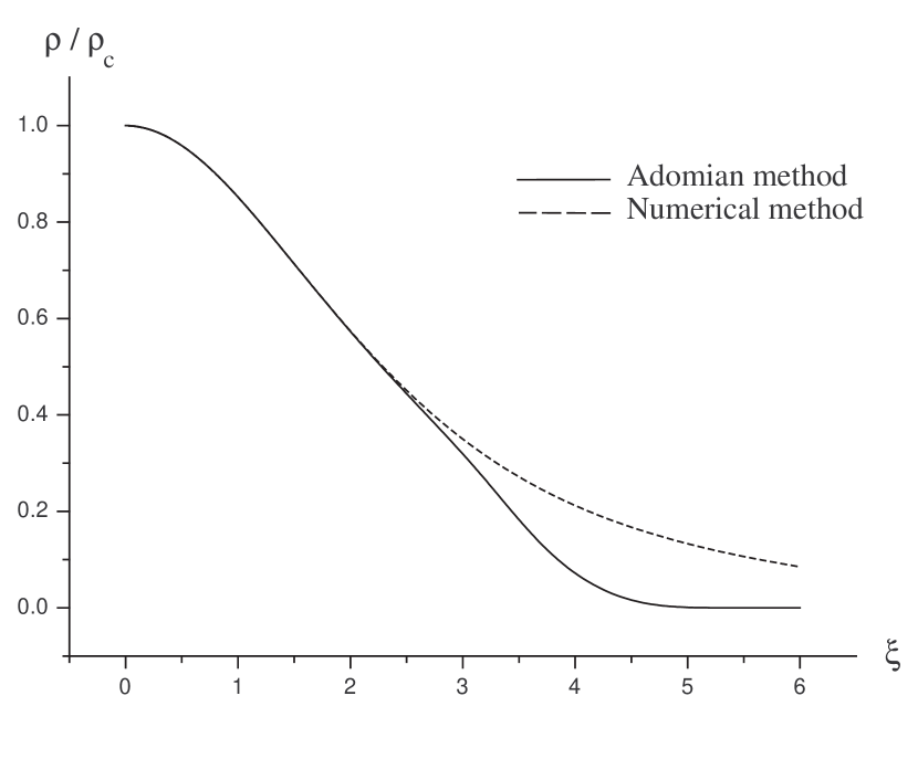
Figure 4: Ratio of density to the central density of an isothermal spherical core in the hydrostatic equilibrium.

References

- (1) Adomian G., 1994, Solving Frontier Problems of Physics: The Decomposition Method, Kluwer Academic Publishers
- (2) Basu S., Ciolek G.E., 2004, ApJ, 607, 39
- (3) Bodenheimer P., Sweigart A., 1968, ApJ, 152, 515
- (4) Cassen P., Moosman A., 1981, Icarus, 48, 353
- (5) Chandrasekhar S., 1939, Introduction to the Study of Stellar Structure, The University of Chicago Press
- (6) Ciolek G.E., Basu S., 2006, ApJ, 652, 442
- (7) Curry C.L., 2002, ApJ, 576, 849
- (8) Curtis E.I., Richer J.S., 2010, MNRAS, 402, 603
- (9) di Francesco J., Evans N.J., Caselli P., Myers P.C., Shirley Y., Aikawa Y., Tafalla M., 2007, prpl.conf., 17
- (10) Fatuzzo M., Adams F.C., Myers P.C., 2004, ApJ, 615, 813
- (11) Galli D., Shu F.H., 1993, Ap.J., 417, 243
- (12) Gammie C.F., Lin Y., Stone J.M., Ostriker E.C., 2003, ApJ, 592, 203
- (13) Goodwin S.P., Ward-Thompson D., Whitworth A.P., 2002, MNRAS, 330, 769
- (14) Hartmann L., 2002, ApJ, 578, 914
- (15) Hartmann L., 2009, Accresion Processes in Astrophysics, 2ed, Cambridge University Press
- (16) Hunter C., 1977, ApJ, 218, 834
- (17) Jones C.E., Basu S., Dubinski J., 2001, ApJ, 551, 387
- (18) Jones C.E., Basu S., 2002, ApJ, 569, 280
- (19) Larson R. B., 1969, MNRAS, 145, 271
- (20) Li P.S., Norman M.L., MacLow M., Heitsch F., 2004, ApJ, 605, 800
- (21) Liao S., 2003, Appl. Math. Comput., 142, 1
- (22) McKee C.F., Ostriker E.C., 2007, ARA & A, 45, 565
- (23) Myers P.C., Fuller G.A., Goodman A.A., Benson P.J., 1991, ApJ, 376, 561
- (24) Offner S.S.R., Krumholz M.R., 2009, ApJ, 693, 914
- (25) Penston M. V., 1969, MNRAS, 144, 425
- (26) Ramos J.I., 2009, Chaos, Solitons & Fractals, 40, 1623
- (27) Shu F., H. 1977, ApJ, 214, 488
- (28) Singh O.P., Pandey R.K., Singh V.K., 2009, Comput. Phys. Comm., 180, 1116
- (29) Tassis K., 2007, MNRAS, 379, 50
- (30) Tassis K., Dowell C.D., Hildebrand R.H., Kirby L., Vaillancourt J.E., 2009, MNRAS, 399, 1681
- (31) Terebey S., Shu F.H., Cassen P., 1984, ApJ, 286, 529
- (32) Ward-Thompson D., André P., Crutcher R., Johnstone D., Onishi T., Wilson C., 2007, prpl.conf., 33
- (33) Wazwaz A.M., 2001, Appl. Math. Comput., 118, 287
(a)
(b)
(a)
(b)
(c)