Searching for the signatures of terrestial planets in solar analogs

Abstract

We present a fully differential chemical abundance analysis using very high-resolution ($\lambda/\delta\lambda\gtrsim 85,000$) and very high signal-to-noise (S/N $\sim 800$ on average) HARPS and UVES spectra of 7 solar twins and 95 solar analogs, 24 are planet hosts and 71 are stars without detected planets. The whole sample of solar analogs provide very accurate Galactic chemical evolution trends in the metalliciy range $-0.3<{\rm[Fe/H]}<0.5$. Solar twins with and without planets show similar mean abundance ratios. We have also analysed a sub-sample of 28 solar analogs, 14 planet hosts and 14 stars without known planets, with spectra at S/N $\sim 850$ on average, in the metallicity range $0.14<{\rm[Fe/H]}<0.36$ and find the same abundance pattern for both samples of stars with and without planets. This result does not depend on either the planet mass, from 7 Earth masses to 17.4 Jupiter masses, or the orbital period of the planets, from 3 to 4300 days. In addition, we have derived the slope of the abundance ratios as a function of the condensation temperature for each star and again find similar distributions of the slopes for both stars with and without planets. In particular, the peaks of these two distributions are placed at a similar value but with opposite sign as that expected from a possible signature of terrestial planets. In particular, two of the planetary systems in this sample, containing each of them a Super-Earth like planet, show slope values very close to these peaks which may suggest that these abundance patterns are not related to the presence of terrestial planets.

1 Introduction

The discovery of first exoplanet orbiting a solar-type star by Mayor & Queloz (1995) initiated a new and very attractive field in which the number of studies is continuously increasing. A substantial amount of spectroscopic data has been collected since then which have allowed to perform not only radial velocity planet searches (see e.g Udry & Santos 2007; Udry & Mayor 2008) but also chemical abundance analysis (e.g Gonzalez et al. 2001; Sadakane et al. 2002; Ecuvillon et al. 2004; Ecuvillon et al. 2006a; Gilli et al. 2006; Neves et al. 2009) and the study of kinematic properties (e.g. Santos et al. 2003; Ecuvillon et al. 2007) trying to focus on finding different signatures able to distiguish stars with and without known planets.

The metal-rich nature of star hosting giant planets was firstly discussed by Gonzalez (1997, 1998) and later on proved by a uniform analysis of large samples of planet-host stars and “single” (hereafter, “single” refers to stars without known planets) stars (Santos et al. 2001). Further studies has confirmed that the probability of finding a planet strongly correlates with the metal content of the parent star (e.g Santos et al. 2004, 2005; Valenti & Fisher 2005; Sousa et al. 2008). Following these studies and using the same spectroscopic data, more complete chemical abundance studies have been done and small differences in some element abundance ratios have been suggested (Bodaghee et al. 2003; Beirão et al. 2005; Gilli et al. 2006; Robinson et al. 2006; Neves et al. 2009), although no definite explanation and/or conclusion has been established yet due to the contradictory results among these studies. See also the reviews on chemical abundance trends in planet-host stars by Israelian (2006, 2007, 2008) and Santos (2006, 2008).

Smith et al. (2001) firstly examined the correlations between the abundance ratio [X/H] as a function of the condensation temperature, $T_{C}$, and they found only six stars among a sample of 20 planet-host stars from Gonzalez et al. (2001) which have positive correlations, suggesting possible accretion of planetesimals. Later on, Ecuvillon et al. (2006b) showed the distributions of the correlation [X/H] versus $T_{C}$ in a sample of 88 planet-host stars and 33 stars without known planets, but they did not find any significant difference between stars with and without planets. However, the effective temperature range in this study was probably too large, $4700\lesssim T_{\rm eff}{\rm[K]}\lesssim 6400$, what may have smoothed out any possible existing signature. Other studies, but on light elements, have been able to find differences between planet hosts and stars without planets (e.g. Israelian et al. 2004; Takeda et al. 2007; Gonzalez et al. 2008). For instance, Israelian et al. (2009) found that apparently Li is always very depleted in solar twins hosting planets whereas this is not the case for similar stars without detected planets. This may suggest that planet formation may alter the Li content of a star. This result has been confirmed by Sousa et al. (2010) and Gonzalez et al. (2010).

Table 1: Spectroscopic observations

Spectrograph	Telescope	Spectral range	$\lambda/\delta\lambda$	Binning	$N_{\rm stars}$	$\mid{\rm S/N}\mid$	$\delta\mid{\rm S/N}\mid$	$\Delta{\rm S/N}$
		[Å]		[Å/pixel]
HARPS	3.6-m	3800–6900	110,000	0.010	85	886	450	370–2020
UVES	VLT	4800–6800	85,000	0.015	8	829	173	550–1100
UES	WHT	4150–7950	33,000	0.040	2	1400	–	–

Note. — Details of the spectroscopic data used in this work. The UVES and UES stars are all planet-hosts. Two of the UVES stars were observed with a slit of $0.3\arcsec$ providing a resolving power $\lambda/\delta\lambda\sim 110,000$.

In the last decade, many studies have addressed the question whether the chemical abundances of the Sun are typical for a solar-type star, i.e. a star of solar mass and age (e.g. Guftafsson et al. 1998; Allende-Prieto et al. 2006). The distribution of spectroscopic metallicities of G-type stars in the solar neighbourhood has been estimated to be $\sim-0.1$ with a typical dispersion of 0.2 dex (e.g. Edvarsson et al. 1993; Allende-Prieto et al. 2004). These authors also found small offsets in some element abundances with respect to their solar values. However, these offsets are not always consistent among different studies which brings some suspicion regarding their existence and size. Allende-Prieto et al. (2006) analyzed a sample of solar analogs and did not find any significant offsets for Si, C, Ca, Ti and Ni, suggesting that the offsets reported in previous studies were likely the result of systematic errors.

Recently, Laws & Gonzalez (2001) performed a differential abundance study of the solar twins 16 Cyg A and 16 Gyg B, i.e. two stars with stellar parameters and metallicities very close to those of the Sun. They used high-quality spectroscopic data of this binary star, and found very small differences in their stellar parameters and Fe abundances. Later on, other authors have proposed and analyzed other solar twins using a similar methodology (see Takeda 2005; Meléndez et al. 2006, 2007). More recently, Meléndez et al. (2009) have studied a sample of 11 solar twins. They also used spectroscopic data at high resolving power, $\lambda/\delta\lambda=65,000$, and high signal-to-noise ratio (S/N $\sim 450$ per pixel). They observed some asteroids to use their spectra as a solar reference. By performing a fully line-by-line differential analysis, they obtained a clear trend, in the mean abundance differences of solar twins with respect to the Sun, $\Delta{\rm[X/Fe]_{SUN-TWINS}}$, as a function of the condensation temperature, $T_{C}$, of the elements. The size of this trend is roughly 0.1 dex and goes from carbon at $\Delta{\rm[C/Fe]}\sim 0.05$ and $T_{C}=40$ K to zirconium at $\Delta{\rm[Zr/Fe]}\sim-0.03$ and $T_{C}=1736$ K. In spite of this tiny signature, they concluded that the most likely explanation to this abundance pattern is related to the presence of terrestial planets in the solar planetary system. Ramírez et al. (2009) confirmed this result on a sample of 64 solar analogs, but with lower signal-to-noise spectra (S/N $\sim 200$), although the correlation was not so clear.

The discovery of more than 400 exoplanets orbiting solar-type stars detected by the radial velocity technique have provided a substantial sample of high-quality spectroscopic data, in particular, the HARPS GTO planet search program which contains so far about 450 stars (see e.g. Neves et al. 2009). The multiplicity of these planetary systems is generating a certain number of questions about the processes of planet formation and evolution (see the introduction in Santos et al. 2010).

In the present study, we will use the high-quality spectroscopic data to get very accurate chemical abundances in a relatively large sample of 95 solar analogs with and without planets, and to examine the results reported in Meléndez et al. (2009).

2 Observations

In this study we have made use of high-resolution spectroscopic data obtained with three different telescopes and instruments: the 3.6-m telescope equipped with HARPS at the Observatorio de La Silla in Chile, the 8.2-m Kueyen VLT (UT2) telescope equipped with UVES at the Observatorio Cerro Paranal in Chile and the 4.2-m WHT telescope equipped with UES at the Observatorio del Roque de los Muchachos in La Palma, Spain. In Table 1, we provide the wavelength ranges, resolving power, S/N and other details of these spectroscopic data.

The data were reduced in a standard manner, and latter normalized within IRAF, using low-order polynomial fits to the observed continuum.

3 Sample

To perform a detailed chemical analysis, we selected stars with S/N $>350$ from these three spectrographs. We end up with a sample of 24 planet-host stars and 71 “single” stars (see Fig. 1). All UVES and UES stars are planet hosts. These 95 solar analogs of the sample have stellar parameters in the ranges $5600<T_{\rm eff}[{\rm K}]<5954$ and $4.0<\log(g[{\rm cm~{}s}^{-2}])<4.6$, and metallicities in the range $-0.3<[{\rm Fe}/{\rm H}]<0.5$ (see Table 2). In Fig. 1, we display the histograms of the effective temperatures, surface gravities and metallicities of the whole sample. The stars hosting planets are more metal-rich than the stars without known planets. Thus, we defined a new sample of metal-rich solar analogs with $0.14<[{\rm Fe}/{\rm H}]<0.36$, containing 14 planet hosts and 14 “single” stars. We have also considered the case of solar twins with and without planets. In that case, the number of stars goes down to only 2 planet-host stars and 5 “single” stars. The ranges of the stellar parameters and metallicities are shown in Table 2.

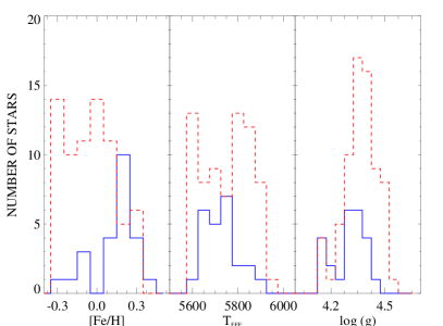
Figure 1: Histograms of the stellar parameters and metallicities of the whole sample of solar analogs hosting planets (solid lines) and without known planets (dashed lines).

Table 2: Ranges of stellar parameters and metallicities in different samples

Samplea	$T_{\mathrm{eff}}$	$\log g$	$\mathrm{[Fe/H]}$	$N_{\rm stars}$b
	[K]	[dex]	[dex]
SA	5600–5954	4.14–4.60	$-0.30$ – $+0.50$	95
mrSA	5600–5954	4.24–4.60	$+0.14$ – $+0.36$	28
ST	5700–5854	4.34–4.54	$-0.07$ – $+0.07$	7

${}^{\rm a}\>$ Stellar samples: solar analogs, “SA”, metal-rich solar analogs, “mrSA”, and solar twins “ST”.

${}^{\rm b}\>$ Total number of stars including those with and without known planets.

4 Stellar Parameters

The stellar parameters and metallicities of the whole sample of stars were computed using the method described in Sousa et al. (2008), based on the equivalent widths (EWs) of 263 Fe I and 36 Fe II lines, measured with the code ARES (Sousa et al. 2007) and evaluating the excitation and ionization equilibria. The chemical abundance derived for each spectral line was computed using the 2002 version of the LTE code MOOG (Sneden 1973), and a grid of Kurucz ATLAS9 plane-parallel model atmospheres (Kurucz 1993). For the HARPS spectra we just adopted the published results in Sousa et al. (2008). For the UVES and UES stars, they had already spectroscopic stellar parameters reported in previous works (see Santos et al. 2004, 2005) computed from a set of 39 Fe I and 12 Fe II and using FEROS, SARG and CORALIE spectra. Therefore, we decided to re-compute the stellar parameters using the higher quality data presented in this study and the method described before. The new stellar parameters are consistent to those in Santos et al. (2004, 2005) although the uncertainties are smaller due to the higher quality of the new data reported in this work. In Table 3 we provide the new stellar parameters of the UVES and UES stars. We note here that the similarities of the parameters of the stars in the sample with respect to the Sun allow us to achieve a high accuracy in the chemical analysis since the possible uncertainties on the atmospheric model and on the stellar parameters and abundances are minimized.

Table 3: Stellar parameters and metallicities from the UVES and UES spectra

HD	$T_{\mathrm{eff}}$	$\delta T_{\mathrm{eff}}$	$\log g$	$\delta\log g$	$\xi_{\rm t}$	$\delta\xi_{\rm t}$	$\mathrm{[Fe/H]}$	$\delta\mathrm{[Fe/H]}$
	[K]	[K]	[dex]	[dex]	[${\rm km}\>{\rm s}^{-1}$]	[${\rm km}\>{\rm s}^{-1}$]	[dex]	[dex]
106252	5880	15	4.40	0.02	1.13	0.02	-0.070	0.011
117207	5680	29	4.34	0.04	1.06	0.04	0.250	0.022
12661	5760	37	4.33	0.07	1.09	0.04	0.385	0.028
216437	5882	21	4.25	0.03	1.25	0.02	0.250	0.018
217107	5679	42	4.32	0.07	1.15	0.05	0.350	0.034
28185	5726	40	4.45	0.05	1.08	0.05	0.230	0.031
4203	5728	49	4.23	0.07	1.18	0.06	0.430	0.036
70642	5732	24	4.42	0.06	1.06	0.03	0.190	0.018
73526	5666	25	4.17	0.04	1.12	0.03	0.260	0.020
76700	5694	27	4.18	0.05	1.05	0.03	0.370	0.023

Note. — Stellar parameters, $T_{\rm eff}\;$and $\log(g/{\rm cm~{}s}^{2})$, microturbulent velocities, $\xi_{\rm t}$, and metallicities , [Fe/H], and their uncertainties, of the planet-host stars observed with UVES/VLT and UES/WHT spectrographs.

5 Chemical abundances

The chemical analysis is done by computing the EWs of spectral lines using the code ARES (Sousa et al. 2007) for most of the elements. We follow the rules given in Sousa et al. (2008) to adjust the ARES parameter $rejt$ for each spectrum taking into account the S/N ratio. We fixed the other ARES parameters to: $smoother=4$, $space=3$, $lineresol=0.07$, $miniline=2$. However, for O, S and Eu, we “manually” determine the EW by integrating the line flux; whereas for Zr, we “manually” performed a gaussian fit taking into account possible blends. In both cases, we use the task splot within the IRAF package. Finally, the EWs of Sr, Ba and Zn lines were checked within IRAF, because, as well as for the elements O, S, Eu and Zr, for some stars, ARES did not find a good fit due to numerical problems and/or bad continuum location. For further details see Sect. 5.2.

Once the EWs are measured, we use the LTE code MOOG (Sneden 1973) to compute the chemical abundance provided by each spectral line, using the appropriate ATLAS model atmosphere of each star. We determine the mean abundance of each element relative to its solar abundance (see Sect. 5.2) by computing the line-by-line mean difference. However, to avoid problems with wrong EW measurements of some spectral lines, we rejected all the lines with an abundance different from the mean abundance by more than a factor of 1.5 times the rms. We also checked that we get the same results when using a factor of 2 times the rms, but we decided to stay in a restrictive position. The line-by-line scatter in the differential abundances goes on average, for the 5 “single” solar twins (see Sect. 6.2), from $\sigma\sim 0.012-0.014$ for elements like Ni, Si and Cr, to $\sigma\sim 0.048-0.056$ for Mg, Zn and Na, whereas for the whole sample of 71 solar analogs without planets, the line-by-line scatter goes on average from $\sigma\sim 0.016$ for elements like Ni, Si and Cr, to $\sigma\sim 0.050$ for Mg and Na and to $\sigma\sim 0.074$ for Zn.

5.1 Atomic data

The oscilator strengths of spectral lines used in this study were extracted from three different works. The line data from Na ($Z=11$) to Ni ($Z=28$) were compiled from Neves et al. (2009). Among these elements, the only element with abundance derived from an ionized state is Sc. C I and S I data is based on Ecuvillon et al. (2004), and [O I] from Ecuvillon et al. (2006a). We note that S I multiplet lines were combined into a single line by adding the $gf$ values. The three Zn I were extracted from Ecuvillon et al. (2004) and Reddy et al. (2003), as well as the four Cu I lines. However, three Cu I lines were rejected high dispersion in the resulting Cu abundances probably due to blending effects with other element lines. The atomic data of the s-process elements Sr, Ba, Y, Zr, Ce, Nd and the r-process element Eu were also extracted from Reddy et al. (2003). Similarly, one Ba I line was discarded since its too high strength provided very different abundance from the other two lines (see Sect. 5.2).

We perform a completely differential analysis to the solar abundances on a line-by-line basis, and therefore, the uncertainties on the oscilator strengths are nearly irrelevant, since most of the lines are in the linear part of the curve of growth, with the exception of some Ba, Fe, and probably also some Zn, Mn, and Ca lines.

5.2 The solar reference

This fully differential analysis is, at least, internally consistent. For this reason, we have used two HARPS solar spectra as solar reference: a daytime sky spectrum (Dall et al. 2006) with a S/N $\sim 1000-1200$ and the spectrum of the Ganymede, a Jupiter’s satellite, with a S/N $\sim 350-400$. However, it should be mentioned that the stars We note here that the spectral lines in solar spectra obtained on the daytime sky are known to exhibit EW and line depth changes (e.g. Gray et al. 2000). Therefore, although the asteroid spectrum has a lower S/N ratio than the sky spectrum, we think it is more likely a better reference solar spectrum and we have adopted the asteroid element abundances as our solar reference in this work. However, we will compare the results obtained with the sky spectrum when analysing the solar twins (see Sect. 6.2), just to show how important is to have a good solar reference spectrum. It should be mentioned, however, that the UVES and UES stars were also analysed using the HARPS Ganymede spectrum as solar reference due to the lack of an appropriate solar spectrum observed with these two instruments.

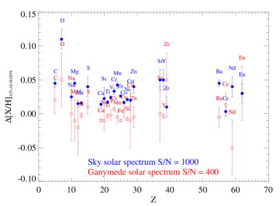
Figure 2: Abundance difference on a line-by-line basis between the Kurucz atlas solar spectrum and, a daytime sky spectrum (filled circles) and a Ganymede spectrum (open circles). The error bars show the standard deviation of the line abundance differences divided by the square root of the number of lines of each element.

In Fig. 2 we display the difference between the solar chemical abundances measured in the Kurucz atlas solar spectrum (Kurucz et al. 1984) and the sky and Ganymede solar HARPS spectra, computed in the same way as the chemical abundances of the whole sample of solar analogs. The abundances of the elements O, Sr, Cu, Eu, Nd, and Zr were determined from only one spectral line; those of the elements C, S, Na, Mg, Al and Ba from 2 lines; those of Zn, Y, Ce from three lines; and the abundances of the rest of elements in Fig. 2 from more than 5 lines. In Fig. 2 we adopt an uncertainty of 0.04 dex and 0.015 dex for the asteroid and sky spectrum, respectively, for the elements with only one line. For the other elements, the adopted uncertainty is computed from the standard deviations of the individual line measurements divided by the square root of the number of lines. Most of the element abundance differences with respect to the Sky HARPS spectrum are slightly higher than zero, whereas these abundance differences are roughly zero in the case of the Ganymede HARPS spectrum. This is probably related to the EW variations in the sky daytime solar HARPS spectrum. In general, elements with relatively small line equivalent widths ($EW\lesssim 10$ mÅ) show the larger discrepancies with the solar atlas abundances. We list below some detailed information on the most problematic elements:

• Oxygen abundance is derived from the forbidden [O I] line at 6300.304 Å (with a expected EW of $\sim 4.1$ mÅ) and is severely blended with the [Ni I] $\lambda$ 6300.34 Å (with a expected EW of $\sim 1.3$ mÅ, e.g. Nissen et al. 2002). In the atlas solar spectrum the whole feature has an EW of $\sim 5.4$ mÅ which provides an abundance, A(O), of 8.74 dex. It is the element with the smaller EW measurement in this study.

• Zirconium abundances come from the line Zr II $\lambda$ 5112.28 Å which slightly blended with two weaker lines. We estimate an EW of $\sim 9.5$ mÅ in the solar atlas spectrum. In the HARPS spectrum of the asteroid, the Zr II abundance is substantially different from that of the atlas spectrum. In addition, the sky and the asteroid spectra show different EW, $\sim$ 9.2 mÅ and 8.6 mÅ, respectively, which translates into an abundance difference of $\sim 0.05$ dex. This does not seems to be related with the S/N ratio, which provides an uncertainty on the EW measurement of $\sim$ 0.05 mÅ and 0.15 mÅ, respectively, from the Cayrel’s formula (Cayrel 1988).

• Neodymium is estimated from the line Nd II $\lambda$ 5092.80 Å which is relatively isolated or weakly blended. However, in this case the sky spectrum clearly show smaller EW than the asteroid spectra, $\sim$ 7.6 mÅ and 9.2 mÅ, respectively, resulting into an abundance difference of $\sim 0.1$ dex.

• Europium is determined from the line Eu II $\lambda$ 6645.13 Å, and is also blended with two lines of smaller EWs. The solar atlas spectrum shows EW of $\sim 6.4$ mÅ.

  

  

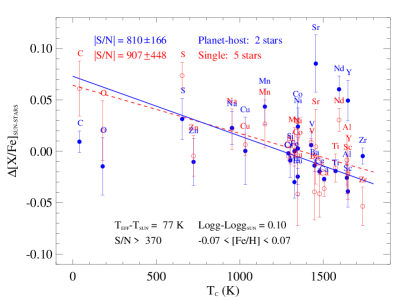
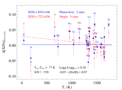
  Figure 3: Mean abundance differences, $\Delta{\rm[X/Fe]_{SUN-STARS}}$, between the Sun, and 2 planet hosts (filled circles) and 5 “single” stars (open circles). Error bars are the standard deviation from the mean divided by the square root of the number of stars. Linear fits to the data points weighted with the error bars are also displayed for planet hosts (solid line) and “single” stars (dashed line). The left panel shows the results using the solar spectrum of the Ganymede and the right panel, using the sky solar spectrum taken in daytime. Note that the average S/N ratios are different in both panel for “single” stars. This is due to the fact that different stars fulfill the [Fe/H] condition of solar twins (see Sect. 6.2).

• Barium, which comes from the two strong lines of Ba II $\lambda$ 5853.69, and $\lambda$ 6496.91 Å, can be easily measured, in principle, although the [Ba II/Fe] versus [Fe/H] trend displays the largest dispersion among the elements analyzed in this work (see Sect. 6.1). This may be related to the dependence of the strong Ba II lines on the microturbulence and other factors.

• Cerium is derived from three lines of Ce II at 4523.08, 4628.16, and 4773.96 Å. The error bars are relatively small but it is also off from the zero level in Fig. 2.

• Strontium and Yttrium abundances are estimated from the relatively strong lines Sr I $\lambda$ 4607.34 Å and the three lines Y II at 5087.43, 5200.42, and 5402.78 Å. As Zr, Ba and Ce, these two elements also show a large dispersion in their Galactic chemical evolution trends (see Sect. 6.1).

6 Discussion

In this section we will discuss the abundance ratios of different elements as a function of the metallicity, [Fe/H], as well as the relation, for different samples of solar analogs, between the abundance difference, $\Delta{\rm[X/Fe]_{SUN-STARS}}$ and the 50% equilibrium condensation temperature, $T_{C}$, for a solar-photosphere composition gas with 50% element condensation, which is the temperature at which half of an element is kept in the gas and the other half is kept into condensates (Lodders 2003).

6.1 Galactic abundance trends

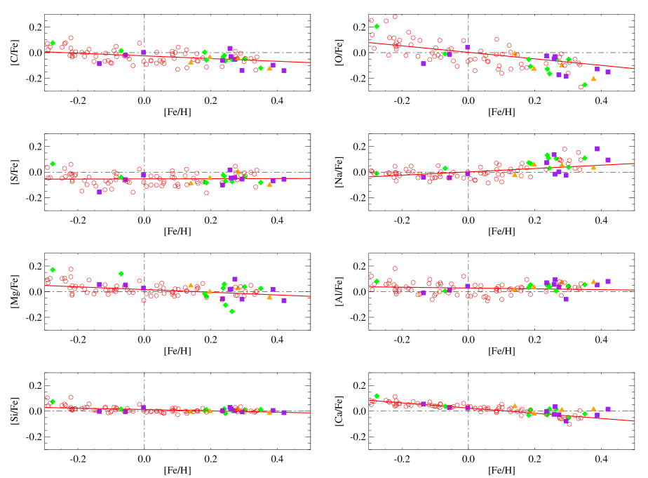
Figure 11: Chemical abundance ratios [X/Fe] versus [Fe/H] for the whole sample of solar analogs, containing 71 “single” stars (open circles) and 24 stars hosting planets, with the most massive planet in an orbital period $P_{\rm orb}<25$ days (filled diamonds), $150<P_{\rm orb}<650$ days (filled squares), $1000<P_{\rm orb}<4300$ days (filled triangles). Solid lines shows linear fits to the data points of the “single” stars.

The high-quality of HARPS and UVES data presented in this work allows us to derive very accurate abundance ratios of many elements. In Figs. 11, 12 and 13 (available online), we show the abundance ratios [X/Fe] versus [Fe/H] for the whole sample of solar analogs analyzed in this work. These trends are compatible with those in previous works (e.g. Bodaghee et al. 2003; Beirão et al. 2005; Bensby et al. 2005; Gilli et al. 2006; Reddy et al. 2006; Takeda 2007; Neves et al. 2009; Ramírez et al. 2009). We note here the low dispersion of most of the elements analyzed in this work, with the exception of some elements discussed in Sect. 5.2. In Table 4 we provide an example of the tables containing all the element abundance ratios [X/Fe] which are all available online.

Table 4: Abundance ratios [X/Fe] of solar analogs without known planets^a

HD	[C/Fe]	[O/Fe]	[S/Fe]	[Na/Fe]	[Mg/Fe]	[Al/Fe]
10180	$0.011\pm 0.035$	$-0.014\pm 0.070$	$0.011\pm 0.021$	$0.071\pm 0.049$	$-0.019\pm 0.078$	$0.006\pm 0.070$
102365	$0.072\pm 0.113$	$0.252\pm 0.070$	$0.037\pm 0.134$	$0.012\pm 0.057$	$0.092\pm 0.014$	$0.122\pm 0.014$
104982	$0.003\pm 0.021$	$-0.022\pm 0.070$	$-0.147\pm 0.134$	$0.023\pm 0.049$	$0.043\pm 0.021$	$0.038\pm 0.042$
106116	$-0.053\pm 0.021$	$-0.018\pm 0.070$	$-0.048\pm 0.014$	$0.012\pm 0.071$	$-0.013\pm 0.064$	$0.027\pm 0.035$
108309	$0.023\pm 0.042$	$0.003\pm 0.070$	$0.023\pm 0.071$	$0.023\pm 0.085$	$0.003\pm 0.071$	$0.023\pm 0.028$
109409	$-0.066\pm 0.021$	$-0.081\pm 0.070$	$-0.016\pm 0.021$	$0.154\pm 0.049$	$-0.021\pm 0.127$	$0.029\pm 0.028$
111031	$-0.045\pm 0.021$	$-0.009\pm 0.070$	$-0.060\pm 0.014$	$0.090\pm 0.014$	$-0.030\pm 0.099$	$-0.030\pm 0.071$
…

${}^{\rm a}\>$ Tables 6, 7, 8, 9, 10, 12, 14, 16 are published in its entirety in the electronic edition of the Astrophysical Journal. A portion is shown here for guidance regarding its form and content.

6.2 HARPS solar twins

We examined the whole sample of HARPS targets trying to search for solar twins defined in the same way as in Meléndez et al. (2009) and we found 2 planet host and 5 “single” stars (see Table 2). In Fig. 3 we display the mean abundance difference, $\Delta{\rm[X/Fe]_{SUN-STARS}}$, versus the condensation temperature, $T_{C}$, for both reference solar spectra, the Ganymede spectrum (left panel) and the daytime sky spectrum (right panel). The main differences between both panels are for the elements O, Nd, Zr, and Y which were discussed in Sect. 5.2. Although the error bars are relatively large to search for any clear trend, it seems that the mean abundance ratios of refratories are on average smaller than those of volatiles. In this plot we also show linear fits to the data points weighted by their error bars. These fits show the decreasing trend of the mean abundance ratios with condensation temperature already reported in Meléndez et al. (2009) but the trend is not so clear. We note here that the S/N is greater than 500 for all stars in this figure, except one “single” star with a S/N $\sim 370$. We display on the upper-right corner of both panels of Fig. 3 the mean S/N and its standard deviation. Besides, the mean S/N ratios are different in both panel for “single” stars. This is due to the fact that just one star in each panel did not fulfill the [Fe/H] condition of solar twins. This is because small offsets in the range 0.01-0.05 dex are found in the differential Fe abundances and probably different Fe lines were used for each star in each case (see Sect. 5). In the right panel of Fig. 3 the fits change completely mainly due to the position of O and Zr abundance ratios. We have checked that expanding the metallicity range up to $\pm 0.15$ dex only increases the number “single” stars, up to 11, which is the same number of stars as in Meléndez et al. (2009). However, this does not change significantly either the position of the data points or the slope of the linear fit.

We find some slight differences between the abundance ratios of stars hosting planets and “single” stars. However, the fits have similar slopes, but only in the left panel of Fig. 3. In addition, the number of planet hosts is too small to allow us to make a strong statement on implications of these differences.

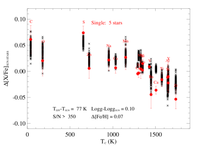
Figure 4: 100 Monte Carlo simulations of the mean element abundance ratios (asterisks) reported in Meléndez et al.(2009) taking into account the error bars shown in Fig. 3, and in comparison with the results (filled circles) shown in Fig. 3.

We have tried to understand why our results do not look like those of Meléndez et al. (2009). Our data has better S/N and resolving power than those of Meléndez et al. but it seems that our dispersion in the mean abundance ratios versus $T_{C}$ and also around the linear fits is larger than in Meléndez et al. (2009). The number of solar twins in our study is smaller, although we think this may not explain the differences between both studies. We have made two Monte Carlo simulations to check if our results are consistent with those of Meléndez et al. (2009), according to our error bars.

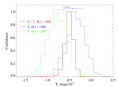
Figure 5: Histograms of slopes of linear fits to 1000 simulations of the points on the fits to mean element abundance ratios reported in Meléndez et al. (2009). The histograms show the distributions for $T_{C}{\rm[K]}<1200$ (dashed line), $T_{C}{\rm[K]}>1200$ (dashed-dotted line), and $0<T_{C}{\rm[K]}<1800$ (solid line). On the top of this figure, we display the slopes and error bars of our results for the 5 “single” twins stars shown in Fig. 3. See also Table 5.

In the first simulation (see Fig. 4), we randomly generate 5 abundance ratios (corresponding to the 5 solar twins) using gaussian distributions around the mean abundance ratios reported in Meléndez et al. (2009) taking into account the error bars displayed in the left panel of Fig. 3. We then compute the mean abundance ratios from these 5 points and finally displayed 100 simulations for each element in Fig. 4 in comparison with our results of the 5 “single” stars (see left panel of Fig. 3). Note that Meléndez et al. (2009) do not include in their analysis the elements Ce, Nd, Sr and Eu, which are in fact some of the outliers in Fig. 2 (see also Sect. 5.2), although they include N, P, and K. This simulation shows that our results and those in Meléndez et al. are indeed consistent, although in some cases only marginally, for most of the elements, according to the error bars shown in Fig. 3, with the exception of Si, Ca and Cu. The line-by line scatter of Ca and Si differential abundances for the 5 “single” stars are on average 0.013 and 0.018 dex whereas the star-to-star scatter, 0.022 and 0.019 dex, respectively. The star-to-star scatter for Cu is 0.027 dex. Note that the error bars in Fig. 3 contain the star-to-star scatter divided by the square root of the number of stars, but only one line of Cu was used in the abundance computation (see Sect. 5.1) The fact that the star-to-star and line-by-line scatters are roughly equal and so small may exacerbate the disagreement between our Ca and Si mean abundances and those in Meléndez et al. (2009). In addition, the scatter of our mean element abundance ratios around the linear fits is higher than in Meléndez et al., which may be related to the solar reference HARPS spectrum used in this analysis.

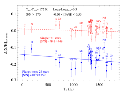
Figure 6: Same as in Fig. 3 but for the mean ratio $\Delta{\rm[X/H]_{SUN-STARS}}$ in the 24 planet host and 71 “single” stars of the whole sample of solar analogs, using the Ganymede spectrum as solar reference.

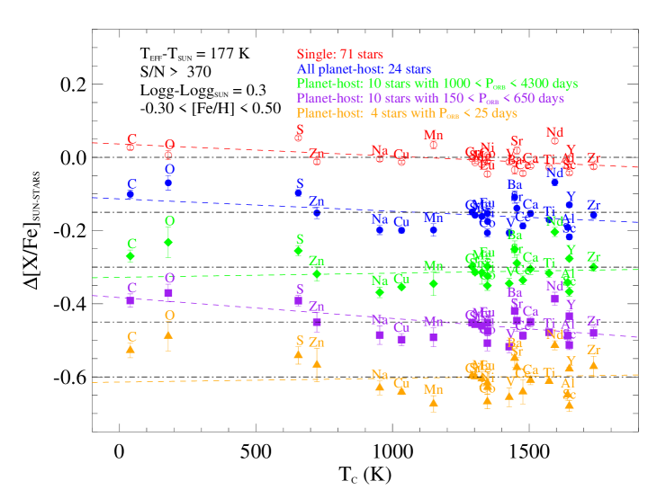
Figure 7: Same as in Fig. 3 containing 71 “single” stars (open circles) and 24 stars hosting planets (filled circles), with the most massive planet in an orbital period $P_{\rm orb}<25$ days (4 stars, filled diamonds), $150<P_{\rm orb}<650$ days (10 stars, filled squares), $1000<P_{\rm orb}<4300$ days (10 stars, filled triangles). The $\Delta{\rm[X/H]_{SUN-STARS}}$ and linear fits has been artificially shifted by $-0.15$ dex, for the sake of clarity. Horizontal dashed-dot lines show the zero point levels for each set of points.

In the second simulation, we derive a linear fit to the mean abundance ratios presented in Meléndez et al. (2009), and define, as new reference abundance ratios, the points on this fit at the condensation temperature of each element. Then we generate, around these new points, abundance ratios using again gaussian distributions which take into account the error bars of the results of “single” stars (see Fig. 3). Finally, for each simulation we perform a linear fit to these abundance ratios. We repeat the same procedure only for elements with $T_{C}$ above or below 1200 K. Three histograms of 1000 simulations are displayed in Fig. 5. The slopes of the linear fits coming from our data are shown on the top of this figure (see also Table 5) and seems to be clearly consistent with the peak of these histograms, although for $T_{C}{\rm[K]}>1200$, our point slightly moves to higher values of the slopes. In Table 5 we provide the values of the slopes in the linear fits to the mean abundance ratios $\Delta{\rm[X/Fe]_{SUN-STARS}}$ as a function of the condensation temperatures $T_{C}$, at different ranges of $T_{C}$.

6.3 All solar analogs

Table 5: Slopes of the linear fit to the mean values $\Delta{\rm[X/Fe]_{SUN-STARS}}$ versus $T_{C}$

Sample	$0<T_{C}[{\rm K}]<1800$	$T_{C}[{\rm K}]<1200$	$T_{C}[{\rm K}]>1200$	$N_{\rm stars}$
sSA	$-0.356\pm 0.032$	$-0.450\pm 0.067$	$-0.468\pm 0.070$	71
pSA	$-0.327\pm 0.051$	$-1.189\pm 0.116$	$-0.281\pm 0.104$	24
smrSA	$-0.235\pm 0.058$	$-1.285\pm 0.119$	$0.179\pm 0.114$	14
pmrSA	$-0.158\pm 0.051$	$-1.596\pm 0.107$	$0.327\pm 0.104$	14
sST	$-0.468\pm 0.090$	$-0.513\pm 0.214$	$-0.306\pm 0.202$	5
pST	$-0.581\pm 0.025$	$0.211\pm 0.147$	$-0.642\pm 0.027$	2
PHs	$0.113\pm 0.069$	$-1.112\pm 0.160$	$0.154\pm 0.144$	4
PHm	$-0.569\pm 0.082$	$-1.112\pm 0.197$	$-0.619\pm 0.167$	10
PHl	$0.102\pm 0.077$	$-1.137\pm 0.192$	$0.299\pm 0.123$	10

Note. — Slopes of the linear fit of the mean abundance ratios, $\Delta{\rm[X/Fe]_{SUN-STARS}}$, as a function of the condensation temperature, $T_{C}$, using the elements with $T_{C}$ within the specified interval, for different stellar samples.

The whole sample of solar analogs presented in this paper contains 24 planet hosts and 71 stars without known planets. In Fig. 6 we display $\Delta{\rm[X/H]_{SUN-STARS}}$ of the sample versus $T_{C}$, only using the Ganymede spectrum as solar reference. The abundance pattern in this figure is very similar to that of $\Delta{\rm[X/Fe]_{SUN-STARS}}$ (see Fig. 7), although due to higher mean metallicity of the stars hosting planets, their mean abundance ratios appear shifted. In addition, the error bars in this plot are larger than in a plot $\Delta{\rm[X/Fe]_{SUN-STARS}}$, since the dispersion in [X/H] is typically larger than in [X/Fe] due to chemical evolution effects. Those elements, like Mn and O, with steeper trends [X/Fe] versus [Fe/H], will show larger abundance differences in the plot $\Delta{\rm[X/Fe]_{SUN-STARS}}$ (see Fig. 7). However, in the plot $\Delta{\rm[X/H]_{SUN-STARS}}$ these differences are relatively smaller and most points seems to agree well with the linear fits. Both stars with and without planets show a similar decreasing trends towards increasing values of $T_{C}$. Nearly equal results are found for the plot $\Delta{\rm[X/Fe]_{SUN-STARS}}$ versus $T_{C}$.

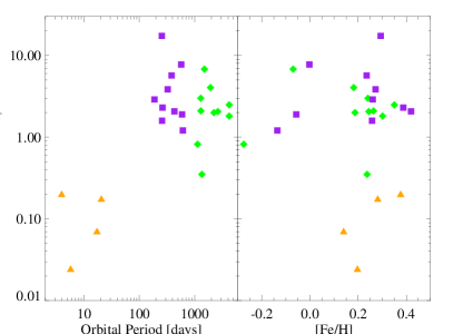
Figure 8: Mass of the most massive planet of each star versus the orbital period of the planet (left panel) and metallicity [Fe/H] (right panel). The symbols as in Fig. 7.

The stars hosting planets studied in this work shows a variety of planetary systems with different orbital periods, $P_{\rm orb}$, from 3 to 4200 days, and minimum masses, i.e. $M_{p}\sin i$, from 0.02 to 17.4 $M_{\rm Jup}$, where $M_{p}$ is the mass of the primary planet, i.e. the most massive planet in the planetary system, $M_{\rm Jup}$, the Jupiter mass, and $i$, the orbital inclination. Among the 24 planet-host stars in the sample, six are planetary systems containing two planets, and one of these planetary systems, in the star HD 160691 ($\mu$ Arae, e.g. Pepe et al. 2007), contains four planets known so far, being the smallest a super-Earth like planet with a minimum mass of $\sim 10.5$ Earth masses and its primary planet a Jupiter-like planet with $M_{p}\sin i\sim 1.8$ $M_{\rm Jup}$ (see the extrasolar-planet encyclopaedia). We do not really know the nature of this and other super-Earth like planets and they may very well be Neptune like ice giants (see e.g. Barnes et al. 2009).

There is only one star, HD 202206, containing a planet with $M_{p}\sin i>10\,M_{\rm Jup}$, which has a primary planet with a $M_{p}\sin i=17.4$ $M_{\rm Jup}$ at $P_{\rm orb}\sim 256$ d, and a secondary planet with a $M_{p}\sin i=2.44$ $M_{\rm Jup}$ at $P_{\rm orb}\sim 1383$ d (e.g. Udry et al. 2002; Correia et al. 2005). This primary planet may be considered as a brown dwarf, whose minimum mass may be settled at $\sim 13$ $M_{\rm Jup}$, and/or entering in the so-called brown dwarf desert (e.g. Halbwachs et al. 2000).

In Fig. 7 we display the mean abundance ratios $\Delta{\rm[X/Fe]_{SUN-STARS}}$ for the 24 stars hosting planets according to the orbital period of the primary planet in the planetary system of each star. We have separated the sample in three ranges: a) 4 stars with primary planets at $P_{\rm orb}[d]<25$; b) 10 stars at $150<P_{\rm orb}[d]<650$; and c) 10 stars at $1000<P_{\rm orb}[d]<4300$. We note that Jupiter has an orbital period of 4333 days around the center-of-mass of the solar system. The distribution of masses of the most massive planet in each planetary system as function of orbital periods and metallicities are shown in Fig. 8. There is no case in this sample in which the most massive planet has orbital period in the gap in between these ranges. Of course, secondary planets in these systems may lie at orbital period within these gaps.

Although the linear fits in Fig. 7 to the element abundance ratios seem to change with the orbital period, the position of most of these abundance ratios remains the same and only few elements like Zn, Nd and Zr modify significantly their position with respect to other elements and thus changing the slope of these fits. We suspect that these changes may be linked to chemical evolution and abundance scatter, and hardly related to the different orbital periods of the primary planets. In Table 5 we give the slopes for the sub-samples of planet-host stars at different ranges of orbital periods. One can appreciate that, due to this large scatter in the mean abundance ratios, the derived slopes are very different for these different sub-samples. However, the number of stars in these different sub-samples is so small that we cannot extract any clear conclusion from this separation in three orbital period intervals.

6.4 Metal-rich solar analogs

To evaluate the abundance trends with the same number of planet hosts and “single” stars, we studied a super-solar metallicity sample of solar analogs with $T_{\rm eff}-T_{\rm eff,\odot}=\pm 177$ K and $\log g-\log g_{\odot}=\pm 0.2$ dex and $0.15\lesssim{\rm[Fe/H]}\lesssim 0.4$. This sample contains 14 stars with and 14 without planets. In Fig. 9, we show the trends $\Delta{\rm[X/Fe]_{\rm SUN-STARS}}$ versus $T_{C}$. The position of some elements in this plot is certainly affected by chemical evolution effects due to the high metal content of the sample, in particular , Mn and O. This may explain the higher scatter of the points in this plot with respect to the linear fits. However, what is relevant from this plot is that both samples of stars with and without planets show almost exactly the same abundance pattern. All the element abundance ratios consistent in both samples within the error bars, except for the Zn, Mn, Ba, and Nd, which still are very close in this plot. In addition, the linear fits have almost exactly the same slope which agrees with the previous statement (see also Table 5). It should be mention that among the stars hosting planets, there is a variety of planetary systems (see Fig. 8) with planets of different masses at different orbital periods. In Sect. 6.5 we provide more details on these planetary systems and discuss the slopes of these trends for each planet-host and “single” star, in the context of the presence of terrestial planets.

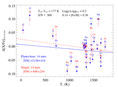
Figure 9: Same as in Fig. 3 for 14 planet host and 14 “single” stars of the sample of metal-rich solar analogs, using the Ganymede spectrum as solar reference.

6.5 Planetary signatures in the abundance trends?

Ecuvillon et al. (2006b) measured the slopes of the trends [X/H] versus $T_{C}$ in a sample of 88 planet-host stars and 33 “single” stars in a large $T_{\rm eff}\;$and [Fe/H] ranges, $4700\lesssim T_{\rm eff}{\rm[K]}\lesssim 6400$ and $-0.8\lesssim{\rm[Fe/H]}\lesssim 0.5$. They did not find any clear difference between these two samples. They also searched for dependence on the planet orbital parameters: mass, orbital period, eccentricity and orbital separation without any success. Ramírez et al. (2009) have derived the slopes in [X/Fe] for two $T_{C}$ ranges above and below 900 K in a sample of solar analogs and twins. There appears to be two distinct groups for super-solar metallicities, showing positive and negative slopes. Following their line of reasoning, a null (solar-like) or even negative slope implies that a great fraction of refractory elements have been extracted from the star-forming cloud to make up dust grains, also suggesting planet formation. Thus, they tentatively conclude that this bimodal distribution of slopes is separating super-solar metallicity stars with and without terrestial planets. Unfortunately, they do not know how many of their stars have planets, whatever their masses are. One should also note that the core of a Jupiter-like planet should contain the same amount refractory elements than roughly three or four terrestial planets. However, Jupiter-like planets also have a substantial amount of volatiles, whereas terrestial planets do trap only refractories.

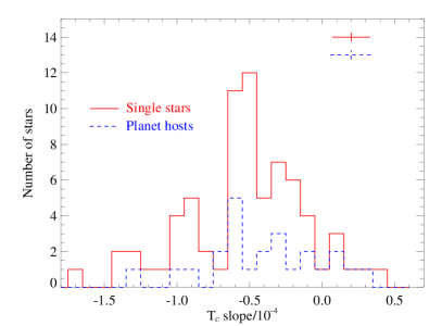
Figure 10: Histograms of slopes of linear fits to 71 “single” stars (solid line) and 24 stars hosting planets (dashed line) of the mean element abundance ratios, $\Delta{\rm[X/Fe]_{SUN-STARS}}$, versus the condensation temperature, $T_{C}$. The mean error bars of the slopes are shown in upper-right corner.

We have determined the slopes of all solar analogs of our sample with and without known planets. In Fig. 10, we display the slopes of the trends $\Delta{\rm[X/Fe]_{\rm SUN-STARS}}$ versus the whole range of $T_{C}$ for all the stars in our sample. We note that the slopes in our study have the same sign than in Meléndez et al. (2009) but opposite than in Ramírez et al. (2009), because the later used the abundance ratios [X/Fe] instead of $\Delta{\rm[X/Fe]_{\rm SUN-STARS}}$. Although the number of planet hosts is smaller than “single” stars, the peak of the distribution of the slopes of these two samples is centered around the same position, which corresponds, in fact, to a negative slope. We may refer here to the Table 5 where we provide the slope of the mean abundance ratios, $\Delta{\rm[X/Fe]_{\rm SUN-STARS}}$, in the whole range of $T_{C}$ of the all solar analogs of our sample with and without known planets. These values are slightly higher than the position of the peaks in Fig. 10 but the values of the slopes are very similar and consistent with the error bars for both stars with and without planets. This indicates that stars with already detected planets behave in similar way, with respect to the chemical abundances, as stars without known planets. In addition, according to the line of reasoning in Ramírez et al., this result also implies that most of the stars with and without planets in our sample would not have terrestial planets. However, in two of them, it has been already detected super-Earth like planets with masses in the range $\sim 7-11$ Earth masses. The most massive one is in the planetary system of the star HD 160691, with a Jupiter-like planet at $P_{\rm orb}\sim 4205$ d and the other one is an isolated planet around the star HD 1461 (e.g. Rivera et al. 2010, see Fig. 8). These two planet-host stars show clearly a negative slope with –0.57 and –0.27 $\times 10^{-4}$ dex/K which is exactly the opposite to what is expected from Ramírez et al. (2009). Positive slopes or consistent with zero within the error bars are found for planet hosts which have either only one Jupiter-like planet at $P_{\rm orb}\gtrsim 1200$ d or three planetary systems with two planets. Two of them, HD 217107 and HD 12661 with two Jupiter-like planets each, at very different orbital periods (e.g. Wright et al. 2009). The other one, HD 47186, contains a Neptune- and a Saturn-like planets at $P_{\rm orb}\sim 4$ and $1354$ d, respectively (Bouchy et al. 2009). We may conclude that there is no reason to expect that these stars hosting relatively massive planets should also contain terrestial planets while the other stars with a already detected super-Earth like planet should not, and/or that the amount of refractory metals in the planet hosts depends only on the amount of terrestial planets. In addition, it seems plausible that many of our targets hosts terrestrial planets. This is supported by numerical simulations which show that terrestrial planets are much more common than giant planets, and probably 80–90% of solar-type stars have terrestrial planets (e.g. Mordasini et al. 2009a,b). This statement agrees with the growing population of low mass planets found in the HARPS sample of exoplanets (see e.g. Udry & Santos 2007).

7 Conclusions

With the aim of investigating possible connection between the abundance pattern versus the condensation temperature, $T_{C}$, and the presence of terrestial planets, we have selected a sample of solar analogs with and without planets from very high signal-to-noise and very high resolution HARPS, UVES and UES spectra. The whole sample contains 71 “single” stars and 24 planet hosts with $5600<T_{\rm eff}[{\rm K}]<5954$, $4.0<\log(g[{\rm cm~{}s}^{-2}])<4.6$, $-0.3<[{\rm Fe}/{\rm H}]<0.5$. We perform a detailed chemical abundance analysis of this sample and investigate possible trends of mean abundance ratios, $\Delta{\rm[X/Fe]_{\rm SUN-STARS}}$, versus $T_{C}$. We find that both stars with and without planets show a similar abundance pattern, except for some elements like Mn which are affected by chemical evolution effects, due to the higher metal content of the stars hosting planets.

Only in the sample of HARPS spectra, there are 7 solar twins, 2 of them hosting planets. We study the mean abundance ratios as a function of $T_{C}$ and compare them with the results of Meléndez et al. (2009). Our results are consistent with their results within our error bars, which has been demonstrated through two Monte Carlo simulations. Nevertheless, the scatter around the linear fits in our data is larger, which may be related to the solar reference HARPS spectrum used in this analysis.

We also select a metal-rich sample of solar analogs in the range $[{\rm Fe}/{\rm H}]=0.25\pm 0.11$ dex. This sample has 14 stars hosting planets and 14 “single” stars. In this case, the abundance pattern and the slope of the linear fit to both samples are almost equal, which may indicate that the abundance pattern found by Meléndez et al. (2009) do not have nothing to do with the presence of planets.

Finally, we derive the slopes of the trend $\Delta{\rm[X/Fe]_{\rm SUN-STARS}}$ versus $T_{C}$ for each star of the whole sample and compare the distribution of the slopes found for stars with and without planets. Although the number of planet hosts is significantly smaller than that of “single” stars, the peaks of the distributions are placed at the same position, at about $-0.5\times 10^{-4}$ dex/K, which is exactly the opposite sign than that required by the presence of terrestial planets, following the line of reasoning in Ramírez et al. (2009). Thus, according to Ramírez et al. (2009), most of our planet-host stars would not contain terrestial planets, a statement that a priori does not appear to be expected.

8 Online Material

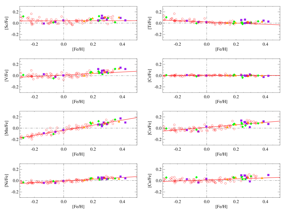
Figure 12: Same as Fig. 11 but for other elements.

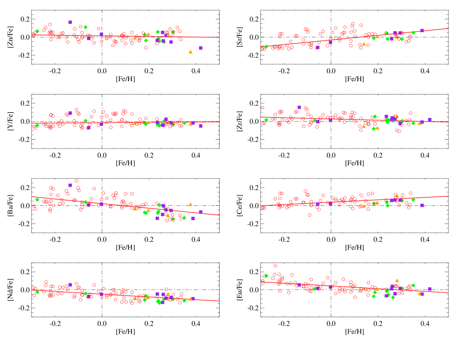
Figure 13: Same as Fig. 11 but for other elements.

Table 6: Abundance ratios [X/Fe] of solar analogs with planets

HD	[C/Fe]	[O/Fe]	[S/Fe]	[Na/Fe]	[Mg/Fe]	[Al/Fe]
102117	$-0.046\pm 0.007$	$-0.101\pm 0.070$	$0.004\pm 0.064$	$0.054\pm 0.035$	$0.024\pm 0.078$	$0.074\pm 0.035$
114729	$0.075\pm 0.028$	$0.206\pm 0.070$	$0.066\pm 0.028$	$-0.009\pm 0.049$	$0.171\pm 0.106$	$0.081\pm 0.035$
134987	$0.032\pm 0.028$	$-0.048\pm 0.070$	$0.017\pm 0.007$	$0.137\pm 0.021$	$0.017\pm 0.078$	$0.057\pm 0.035$
1461	$-0.037\pm 0.028$	$-0.127\pm 0.070$	$-0.047\pm 0.070$	$0.058\pm 0.049$	$-0.002\pm 0.049$	$0.033\pm 0.028$
160691	$-0.047\pm 0.007$	$-0.052\pm 0.070$	$-0.037\pm 0.021$	$0.038\pm 0.113$	$0.038\pm 0.042$	$0.043\pm 0.035$
16417	$-0.080\pm 0.028$	$-0.010\pm 0.070$	$-0.090\pm 0.042$	$-0.025\pm 0.106$	$0.045\pm 0.035$	$0.015\pm 0.035$
196050	$-0.021\pm 0.028$	$0.159\pm 0.070$	$-0.031\pm 0.042$	$0.109\pm 0.071$	$0.059\pm 0.014$	$0.059\pm 0.028$
202206	$-0.139\pm 0.007$	$-0.184\pm 0.070$	$-0.054\pm 0.014$	$-0.024\pm 0.099$	$-0.059\pm 0.078$	$-0.059\pm 0.035$
204313	$0.003\pm 0.035$	$-0.052\pm 0.070$	$-0.077\pm 0.078$	$0.073\pm 0.064$	$-0.017\pm 0.064$	$0.033\pm 0.021$
20782	$-0.018\pm 0.021$	$-0.013\pm 0.070$	$-0.058\pm 0.064$	$-0.043\pm 0.042$	$0.052\pm 0.064$	$0.012\pm 0.035$
222582	$0.002\pm 0.028$	$0.043\pm 0.070$	$-0.023\pm 0.021$	$-0.012\pm 0.021$	$0.027\pm 0.007$	$0.043\pm 0.042$
47186	$-0.032\pm 0.021$	$-0.127\pm 0.070$	$-0.022\pm 0.007$	$0.133\pm 0.028$	$0.028\pm 0.035$	$0.048\pm 0.035$
65216	$-0.085\pm 0.014$	$-0.085\pm 0.070$	$-0.155\pm 0.028$	$-0.040\pm 0.021$	$0.055\pm 0.070$	$-0.010\pm 0.021$
92788	$-0.052\pm 0.028$	$-0.172\pm 0.070$	$-0.042\pm 0.070$	$0.003\pm 0.134$	$0.098\pm 0.085$	$0.038\pm 0.028$
106252	$0.015\pm 0.035$	$-0.010\pm 0.070$	$-0.040\pm 0.042$	$0.030\pm 0.057$	$0.140\pm 0.070$	$0.005\pm 0.035$
117207	$-0.064\pm 0.028$	$-0.164\pm 0.070$	$-0.069\pm 0.021$	$0.031\pm 0.120$	$-0.104\pm 0.070$	$0.036\pm 0.028$
12661	$-0.097\pm 0.070$	$-0.127\pm 0.070$	$-0.067\pm 0.028$	$0.183\pm 0.028$	$0.018\pm 0.120$	$0.053\pm 0.014$
216437	$-0.054\pm 0.028$	$-0.054\pm 0.070$	$-0.074\pm 0.028$	$0.106\pm 0.042$	$-0.154\pm 0.070$	$0.006\pm 0.070$
217107	$-0.120\pm 0.070$	$-0.250\pm 0.070$	$-0.080\pm 0.014$	$0.110\pm 0.028$	$0.025\pm 0.120$	$0.055\pm 0.035$
28185	$-0.060\pm 0.007$	$-0.025\pm 0.070$	$-0.100\pm 0.064$	$0.075\pm 0.085$	$-0.055\pm 0.070$	$0.070\pm 0.021$
4203	$-0.140\pm 0.070$	$-0.150\pm 0.070$	$-0.055\pm 0.035$	$0.095\pm 0.092$	$-0.070\pm 0.070$	$0.080\pm 0.028$
70642	$-0.057\pm 0.014$	$-0.107\pm 0.070$	$-0.082\pm 0.021$	$0.068\pm 0.078$	$-0.037\pm 0.070$	$0.053\pm 0.028$
73526	$-0.031\pm 0.028$	$-0.031\pm 0.070$	$-0.046\pm 0.021$	$-0.016\pm 0.120$	$0.019\pm 0.070$	$0.094\pm 0.035$
76700	$-0.127\pm 0.028$	$-0.207\pm 0.070$	$-0.102\pm 0.021$	$0.033\pm 0.028$	$-0.047\pm 0.070$	$0.073\pm 0.042$

Table 7: Abundance ratios [X/Fe] of solar analogs with planets

HD	[Si/Fe]	[Ca/Fe]	[Sc/Fe]	[Ti/Fe]	[V/Fe]	[Cr/Fe]
102117	$0.018\pm 0.020$	$0.007\pm 0.062$	$0.101\pm 0.061$	$0.021\pm 0.036$	$0.059\pm 0.021$	$-0.012\pm 0.024$
114729	$0.074\pm 0.017$	$0.118\pm 0.032$	$0.120\pm 0.026$	$0.104\pm 0.024$	$0.012\pm 0.038$	$0.009\pm 0.023$
134987	$0.029\pm 0.027$	$-0.025\pm 0.032$	$0.087\pm 0.055$	$-0.001\pm 0.033$	$0.050\pm 0.015$	$0.002\pm 0.022$
1461	$-0.002\pm 0.021$	$-0.021\pm 0.055$	$0.083\pm 0.029$	$0.004\pm 0.015$	$0.048\pm 0.026$	$-0.000\pm 0.009$
160691	$0.008\pm 0.016$	$-0.051\pm 0.055$	$0.091\pm 0.052$	$0.010\pm 0.030$	$0.046\pm 0.021$	$0.007\pm 0.017$
16417	$-0.005\pm 0.012$	$0.038\pm 0.046$	$0.035\pm 0.029$	$0.000\pm 0.019$	$-0.005\pm 0.023$	$0.002\pm 0.013$
196050	$0.018\pm 0.020$	$-0.017\pm 0.028$	$0.123\pm 0.049$	$0.011\pm 0.016$	$0.044\pm 0.019$	$0.001\pm 0.021$
202206	$-0.005\pm 0.032$	$-0.077\pm 0.033$	$0.064\pm 0.047$	$0.003\pm 0.027$	$0.059\pm 0.028$	$0.021\pm 0.019$
204313	$0.004\pm 0.014$	$-0.032\pm 0.036$	$0.064\pm 0.047$	$-0.008\pm 0.019$	$0.054\pm 0.009$	$0.001\pm 0.009$
20782	$-0.004\pm 0.009$	$0.029\pm 0.016$	$0.021\pm 0.044$	$0.020\pm 0.017$	$-0.021\pm 0.022$	$0.002\pm 0.013$
222582	$0.028\pm 0.014$	$0.025\pm 0.013$	$0.051\pm 0.028$	$0.019\pm 0.014$	$0.004\pm 0.015$	$0.002\pm 0.008$
47186	$0.008\pm 0.027$	$-0.028\pm 0.037$	$0.040\pm 0.045$	$0.007\pm 0.019$	$0.074\pm 0.041$	$0.001\pm 0.017$
65216	$-0.003\pm 0.013$	$0.055\pm 0.016$	$-0.007\pm 0.027$	$0.042\pm 0.014$	$0.025\pm 0.012$	$0.010\pm 0.005$
92788	$0.003\pm 0.020$	$-0.027\pm 0.050$	$0.090\pm 0.055$	$0.005\pm 0.024$	$0.093\pm 0.032$	$-0.003\pm 0.013$
106252	$0.016\pm 0.005$	$0.037\pm 0.016$	$0.012\pm 0.017$	$-0.003\pm 0.018$	$-0.048\pm 0.025$	$-0.013\pm 0.010$
117207	$-0.018\pm 0.017$	$0.017\pm 0.029$	$0.048\pm 0.031$	$-0.016\pm 0.026$	$0.051\pm 0.043$	$-0.036\pm 0.010$
12661	$0.006\pm 0.055$	$-0.032\pm 0.046$	$0.093\pm 0.083$	$0.046\pm 0.051$	$0.141\pm 0.061$	$-0.024\pm 0.048$
216437	$0.003\pm 0.016$	$0.016\pm 0.038$	$0.084\pm 0.051$	$0.001\pm 0.030$	$0.026\pm 0.009$	$-0.006\pm 0.016$
217107	$0.013\pm 0.051$	$-0.022\pm 0.037$	$0.016\pm 0.084$	$0.033\pm 0.063$	$0.120\pm 0.025$	$0.002\pm 0.052$
28185	$0.004\pm 0.027$	$-0.002\pm 0.041$	$0.050\pm 0.033$	$0.056\pm 0.033$	$0.117\pm 0.019$	$0.008\pm 0.027$
4203	$-0.012\pm 0.020$	$0.015\pm 0.036$	$0.050\pm 0.042$	$0.028\pm 0.061$	$0.118\pm 0.048$	$-0.003\pm 0.024$
70642	$0.011\pm 0.023$	$0.008\pm 0.037$	$0.070\pm 0.033$	$0.027\pm 0.030$	$0.065\pm 0.026$	$0.017\pm 0.013$
73526	$0.016\pm 0.026$	$0.036\pm 0.030$	$0.132\pm 0.031$	$0.062\pm 0.043$	$0.088\pm 0.035$	$-0.001\pm 0.007$
76700	$-0.014\pm 0.026$	$0.013\pm 0.034$	$0.099\pm 0.069$	$0.023\pm 0.052$	$0.121\pm 0.036$	$-0.004\pm 0.026$

Table 8: Abundance ratios [X/Fe] of solar analogs with planets

HD	[Mn/Fe]	[Co/Fe]	[Ni/Fe]	[Cu/Fe]	[Zn/Fe]	[Sr/Fe]
102117	$0.079\pm 0.043$	$0.099\pm 0.042$	$0.040\pm 0.025$	$0.049\pm 0.070$	$0.024\pm 0.078$	$-0.001\pm 0.070$
114729	$-0.172\pm 0.061$	$-0.006\pm 0.026$	$-0.031\pm 0.019$	$0.056\pm 0.070$	$0.066\pm 0.127$	$-0.104\pm 0.070$
134987	$0.062\pm 0.068$	$0.109\pm 0.012$	$0.055\pm 0.017$	$0.092\pm 0.070$	$0.052\pm 0.057$	$-0.018\pm 0.070$
1461	$0.093\pm 0.016$	$0.060\pm 0.020$	$0.038\pm 0.016$	$0.053\pm 0.070$	$0.028\pm 0.106$	$0.003\pm 0.070$
160691	$0.098\pm 0.029$	$0.078\pm 0.018$	$0.031\pm 0.027$	$0.078\pm 0.070$	$0.058\pm 0.057$	$-0.022\pm 0.070$
16417	$0.010\pm 0.020$	$0.015\pm 0.017$	$0.004\pm 0.016$	$0.020\pm 0.070$	$-0.015\pm 0.064$	$-0.080\pm 0.070$
196050	$0.069\pm 0.016$	$0.074\pm 0.021$	$0.043\pm 0.014$	$0.069\pm 0.070$	$-0.016\pm 0.021$	$-0.021\pm 0.070$
202206	$0.070\pm 0.042$	$0.017\pm 0.054$	$0.029\pm 0.017$	$-0.014\pm 0.070$	$-0.054\pm 0.127$	$0.046\pm 0.070$
204313	$0.098\pm 0.018$	$0.063\pm 0.024$	$0.033\pm 0.018$	$0.058\pm 0.070$	$0.028\pm 0.113$	$-0.012\pm 0.070$
20782	$-0.066\pm 0.039$	$-0.059\pm 0.021$	$-0.041\pm 0.013$	$-0.033\pm 0.070$	$-0.013\pm 0.070$	$-0.113\pm 0.070$
222582	$-0.032\pm 0.019$	$0.028\pm 0.011$	$-0.005\pm 0.014$	$0.032\pm 0.070$	$0.032\pm 0.057$	$-0.057\pm 0.070$
47186	$0.123\pm 0.034$	$0.093\pm 0.024$	$0.053\pm 0.019$	$0.063\pm 0.070$	$0.058\pm 0.134$	$0.043\pm 0.070$
65216	$-0.090\pm 0.007$	$-0.033\pm 0.008$	$-0.040\pm 0.021$	$0.025\pm 0.070$	$0.165\pm 0.070$	–
92788	$0.100\pm 0.035$	$0.081\pm 0.019$	$0.054\pm 0.022$	$0.048\pm 0.070$	$0.018\pm 0.042$	$0.048\pm 0.070$
106252	$-0.105\pm 0.049$	$-0.028\pm 0.008$	$-0.010\pm 0.013$	$0.060\pm 0.070$	$0.110\pm 0.070$	–
117207	$0.061\pm 0.092$	$0.024\pm 0.019$	$0.017\pm 0.022$	$0.026\pm 0.070$	$-0.044\pm 0.070$	–
12661	$0.173\pm 0.036$	$0.120\pm 0.021$	$0.072\pm 0.035$	–	–	$0.073\pm 0.070$
216437	$0.051\pm 0.021$	$0.046\pm 0.014$	$0.026\pm 0.027$	$0.026\pm 0.070$	$-0.054\pm 0.070$	–
217107	$0.152\pm 0.021$	$0.085\pm 0.037$	$0.039\pm 0.034$	–	–	$0.050\pm 0.070$
28185	$0.065\pm 0.071$	$0.135\pm 0.028$	$0.056\pm 0.033$	$0.095\pm 0.070$	$-0.035\pm 0.070$	–
4203	$0.100\pm 0.071$	$0.074\pm 0.110$	$0.042\pm 0.040$	$0.100\pm 0.070$	$-0.120\pm 0.070$	–
70642	$0.078\pm 0.049$	$0.077\pm 0.018$	$0.044\pm 0.014$	$0.053\pm 0.070$	$-0.037\pm 0.070$	–
73526	$0.034\pm 0.092$	$0.105\pm 0.026$	$0.026\pm 0.025$	$0.089\pm 0.070$	$-0.041\pm 0.070$	–
76700	$0.113\pm 0.028$	$0.097\pm 0.036$	$0.030\pm 0.032$	$0.043\pm 0.070$	$-0.167\pm 0.070$	–

Table 9: Abundance ratios [X/Fe] of solar analogs with planets

HD	[Y/Fe]	[Zr/Fe]	[Ba/Fe]	[Ce/Fe]	[Nd/Fe]	[Eu/Fe]
102117	$-0.015\pm 0.049$	$0.049\pm 0.070$	$-0.116\pm 0.134$	$0.104\pm 0.078$	$-0.051\pm 0.070$	$0.099\pm 0.070$
114729	$-0.044\pm 0.035$	$0.016\pm 0.070$	$0.066\pm 0.099$	–	$-0.025\pm 0.070$	$0.155\pm 0.070$
134987	$-0.038\pm 0.061$	$0.022\pm 0.070$	$-0.098\pm 0.070$	$0.057\pm 0.078$	$-0.138\pm 0.070$	$0.012\pm 0.070$
1461	$-0.017\pm 0.052$	$-0.077\pm 0.070$	$-0.057\pm 0.070$	$0.028\pm 0.078$	$-0.087\pm 0.070$	$0.003\pm 0.070$
160691	$-0.032\pm 0.069$	$-0.002\pm 0.070$	$-0.147\pm 0.148$	$0.053\pm 0.035$	$-0.102\pm 0.070$	$0.018\pm 0.070$
16417	$-0.023\pm 0.021$	$-0.060\pm 0.070$	$-0.040\pm 0.028$	$-0.010\pm 0.070$	$-0.100\pm 0.070$	$0.010\pm 0.070$
196050	$-0.014\pm 0.021$	$-0.011\pm 0.070$	$-0.066\pm 0.007$	$-0.001\pm 0.042$	$-0.121\pm 0.070$	$-0.001\pm 0.070$
202206	$-0.014\pm 0.035$	$-0.024\pm 0.070$	$-0.054\pm 0.014$	$0.061\pm 0.148$	$-0.084\pm 0.070$	$0.016\pm 0.070$
204313	$-0.018\pm 0.047$	$-0.082\pm 0.070$	$-0.077\pm 0.021$	$0.023\pm 0.078$	$-0.112\pm 0.070$	$-0.072\pm 0.070$
20782	$-0.070\pm 0.023$	$-0.003\pm 0.070$	$0.007\pm 0.014$	$0.017\pm 0.014$	$-0.073\pm 0.070$	$0.017\pm 0.070$
222582	$-0.031\pm 0.021$	$0.012\pm 0.070$	$0.018\pm 0.007$	$0.022\pm 0.014$	$-0.047\pm 0.070$	$0.032\pm 0.070$
47186	$-0.041\pm 0.042$	$0.013\pm 0.070$	$-0.082\pm 0.007$	$0.038\pm 0.120$	$-0.127\pm 0.070$	$-0.017\pm 0.070$
65216	$0.092\pm 0.012$	$0.155\pm 0.070$	$0.225\pm 0.014$	–	$0.055\pm 0.070$	$0.055\pm 0.070$
92788	$0.024\pm 0.012$	$0.028\pm 0.070$	$-0.047\pm 0.007$	$0.063\pm 0.120$	$-0.092\pm 0.070$	$-0.042\pm 0.070$
106252	$0.007\pm 0.047$	$0.010\pm 0.070$	$0.040\pm 0.071$	–	$-0.040\pm 0.070$	$0.010\pm 0.070$
117207	$-0.048\pm 0.023$	$0.016\pm 0.070$	$0.006\pm 0.127$	–	$-0.144\pm 0.070$	$-0.054\pm 0.070$
12661	$-0.017\pm 0.020$	$-0.007\pm 0.070$	$-0.142\pm 0.021$	$0.003\pm 0.071$	$-0.097\pm 0.070$	$-0.047\pm 0.070$
216437	$0.003\pm 0.049$	$0.006\pm 0.070$	$-0.014\pm 0.071$	–	$-0.104\pm 0.070$	$-0.084\pm 0.070$
217107	$-0.017\pm 0.035$	$-0.020\pm 0.070$	$-0.135\pm 0.007$	$0.065\pm 0.035$	$-0.120\pm 0.070$	$0.050\pm 0.070$
28185	$-0.012\pm 0.021$	$0.055\pm 0.070$	$-0.140\pm 0.021$	–	$-0.045\pm 0.070$	$-0.065\pm 0.070$
4203	$-0.050\pm 0.026$	$0.020\pm 0.070$	$-0.070\pm 0.028$	–	–	$0.010\pm 0.070$
70642	$-0.030\pm 0.042$	$0.053\pm 0.070$	$-0.082\pm 0.021$	–	$-0.067\pm 0.070$	$-0.027\pm 0.070$
73526	$-0.044\pm 0.025$	$0.039\pm 0.070$	$-0.001\pm 0.014$	–	$-0.051\pm 0.070$	$0.039\pm 0.070$
76700	$-0.033\pm 0.006$	$-0.027\pm 0.070$	$0.008\pm 0.007$	–	$-0.107\pm 0.070$	$-0.047\pm 0.070$

Table 10: Abundance ratios [X/Fe] of solar analogs without known planets

HD	[C/Fe]	[O/Fe]	[S/Fe]	[Na/Fe]	[Mg/Fe]	[Al/Fe]
10180	$0.011\pm 0.035$	$-0.014\pm 0.070$	$0.011\pm 0.021$	$0.071\pm 0.049$	$-0.019\pm 0.078$	$0.006\pm 0.070$
102365	$0.072\pm 0.113$	$0.252\pm 0.070$	$0.037\pm 0.134$	$0.012\pm 0.057$	$0.092\pm 0.014$	$0.122\pm 0.014$
104982	$0.003\pm 0.021$	$-0.022\pm 0.070$	$-0.147\pm 0.134$	$0.023\pm 0.049$	$0.043\pm 0.021$	$0.038\pm 0.042$
106116	$-0.053\pm 0.021$	$-0.018\pm 0.070$	$-0.048\pm 0.014$	$0.012\pm 0.071$	$-0.013\pm 0.064$	$0.027\pm 0.035$
108309	$0.023\pm 0.042$	$0.003\pm 0.070$	$0.023\pm 0.071$	$0.023\pm 0.085$	$0.003\pm 0.071$	$0.023\pm 0.028$
109409	$-0.066\pm 0.021$	$-0.081\pm 0.070$	$-0.016\pm 0.021$	$0.154\pm 0.049$	$-0.021\pm 0.127$	$0.029\pm 0.028$
111031	$-0.045\pm 0.021$	$-0.009\pm 0.070$	$-0.060\pm 0.014$	$0.090\pm 0.014$	$-0.030\pm 0.099$	$-0.030\pm 0.071$
114853	$-0.021\pm 0.035$	$0.114\pm 0.070$	$-0.016\pm 0.014$	$-0.041\pm 0.049$	$0.029\pm 0.007$	$0.054\pm 0.028$
11505	$0.116\pm 0.035$	$0.281\pm 0.070$	$0.061\pm 0.042$	$0.046\pm 0.035$	$0.176\pm 0.035$	$0.181\pm 0.028$
117105	$0.043\pm 0.014$	$0.033\pm 0.070$	$-0.042\pm 0.049$	$-0.012\pm 0.035$	$0.103\pm 0.057$	$0.058\pm 0.007$
126525	$0.016\pm 0.007$	$-0.019\pm 0.070$	$0.001\pm 0.071$	$0.051\pm 0.042$	$0.006\pm 0.049$	$0.056\pm 0.021$
134606	$0.011\pm 0.021$	$-0.034\pm 0.070$	$0.046\pm 0.042$	$0.101\pm 0.021$	$0.036\pm 0.042$	$0.076\pm 0.028$
134664	$-0.130\pm 0.028$	$-0.160\pm 0.070$	$-0.095\pm 0.078$	$-0.075\pm 0.092$	$-0.030\pm 0.014$	$-0.060\pm 0.071$
13724	$-0.109\pm 0.021$	$-0.084\pm 0.070$	$-0.084\pm 0.028$	$0.021\pm 0.064$	$-0.064\pm 0.071$	$0.001\pm 0.035$
1388	$-0.068\pm 0.028$	$-0.068\pm 0.070$	$-0.078\pm 0.085$	$0.002\pm 0.042$	$-0.068\pm 0.099$	$-0.033\pm 0.007$
140901	$-0.045\pm 0.007$	$-0.130\pm 0.070$	$-0.045\pm 0.035$	$-0.015\pm 0.049$	$-0.035\pm 0.049$	$0.040\pm 0.028$
144585	$-0.135\pm 0.014$	$-0.095\pm 0.070$	$-0.115\pm 0.057$	$0.020\pm 0.064$	$-0.000\pm 0.064$	$0.020\pm 0.007$
145809	$0.042\pm 0.035$	$0.247\pm 0.070$	$-0.048\pm 0.078$	$-0.013\pm 0.042$	$0.102\pm 0.021$	$0.057\pm 0.028$
146233	$-0.072\pm 0.014$	$-0.022\pm 0.070$	$-0.108\pm 0.035$	$-0.012\pm 0.057$	$0.067\pm 0.071$	$-0.037\pm 0.007$
154962	$-0.046\pm 0.035$	$-0.051\pm 0.070$	$-0.001\pm 0.014$	$0.029\pm 0.071$	$0.049\pm 0.070$	$0.034\pm 0.021$
157347	$-0.065\pm 0.021$	$-0.140\pm 0.070$	$-0.100\pm 0.014$	$-0.060\pm 0.042$	$0.005\pm 0.035$	$0.050\pm 0.028$
161612	$-0.064\pm 0.007$	$-0.089\pm 0.070$	$-0.074\pm 0.035$	$-0.029\pm 0.071$	$0.041\pm 0.014$	$0.036\pm 0.007$
171665	$-0.050\pm 0.007$	$-0.065\pm 0.070$	$-0.080\pm 0.021$	$0.000\pm 0.049$	$-0.005\pm 0.042$	$0.030\pm 0.021$
177409	$-0.101\pm 0.021$	$-0.106\pm 0.070$	$-0.156\pm 0.085$	$-0.031\pm 0.049$	$-0.006\pm 0.070$	$-0.026\pm 0.014$
177565	$-0.020\pm 0.035$	$0.105\pm 0.070$	$-0.010\pm 0.007$	$0.020\pm 0.064$	$-0.000\pm 0.049$	$0.025\pm 0.028$
183658	$-0.082\pm 0.134$	$-0.347\pm 0.070$	$-0.101\pm 0.092$	$0.039\pm 0.064$	$-0.032\pm 0.049$	$0.014\pm 0.070$
188748	$-0.067\pm 0.078$	–	$-0.137\pm 0.106$	$-0.017\pm 0.078$	$0.053\pm 0.007$	$0.063\pm 0.021$
189567	$0.077\pm 0.028$	$0.117\pm 0.070$	$-0.033\pm 0.014$	$-0.008\pm 0.021$	$0.082\pm 0.021$	$0.087\pm 0.028$
189625	$-0.112\pm 0.007$	$0.173\pm 0.070$	$-0.162\pm 0.049$	$-0.037\pm 0.099$	$-0.047\pm 0.071$	$-0.022\pm 0.021$
190248	$-0.034\pm 0.007$	$-0.269\pm 0.070$	$0.016\pm 0.021$	$0.096\pm 0.021$	$0.001\pm 0.127$	$0.061\pm 0.028$
199190	$-0.008\pm 0.042$	$0.462\pm 0.070$	$-0.008\pm 0.057$	$0.037\pm 0.021$	$0.022\pm 0.028$	$0.007\pm 0.035$
203432	$-0.070\pm 0.070$	$-0.160\pm 0.070$	$-0.005\pm 0.035$	$0.065\pm 0.064$	$-0.035\pm 0.106$	$0.040\pm 0.028$
20619	$-0.033\pm 0.014$	$0.027\pm 0.070$	$-0.073\pm 0.127$	$-0.013\pm 0.042$	$-0.018\pm 0.021$	$-0.018\pm 0.021$
207129	$-0.091\pm 0.021$	$-0.056\pm 0.070$	$-0.111\pm 0.021$	$-0.051\pm 0.035$	$-0.016\pm 0.070$	$-0.036\pm 0.028$
20807	$0.036\pm 0.035$	$0.061\pm 0.070$	$-0.009\pm 0.042$	$-0.004\pm 0.064$	$0.116\pm 0.120$	$0.016\pm 0.021$
208704	$-0.009\pm 0.007$	$0.096\pm 0.070$	$-0.059\pm 0.021$	$-0.014\pm 0.042$	$0.001\pm 0.035$	$0.001\pm 0.021$

Table 11: Continued.

HD	[C/Fe]	[O/Fe]	[S/Fe]	[Na/Fe]	[Mg/Fe]	[Al/Fe]
210918	$0.050\pm 0.035$	$0.175\pm 0.070$	$-0.035\pm 0.028$	$-0.035\pm 0.028$	$0.020\pm 0.078$	$0.070\pm 0.007$
212708	$-0.030\pm 0.007$	$-0.075\pm 0.070$	$-0.005\pm 0.014$	$0.095\pm 0.028$	$-0.030\pm 0.120$	$0.055\pm 0.028$
221146	$0.002\pm 0.007$	$-0.103\pm 0.070$	$-0.108\pm 0.120$	$0.057\pm 0.057$	$0.022\pm 0.035$	$0.007\pm 0.028$
222595	$-0.060\pm 0.042$	$-0.050\pm 0.070$	$-0.030\pm 0.028$	$-0.065\pm 0.049$	$-0.035\pm 0.035$	$-0.025\pm 0.007$
222669	$-0.058\pm 0.014$	$-0.068\pm 0.070$	$-0.087\pm 0.014$	$-0.003\pm 0.035$	$0.027\pm 0.078$	$-0.072\pm 0.007$
223171	$-0.008\pm 0.035$	$0.057\pm 0.070$	$-0.028\pm 0.021$	$0.002\pm 0.106$	$0.032\pm 0.049$	$0.017\pm 0.028$
27063	$-0.084\pm 0.007$	$-0.069\pm 0.070$	$-0.074\pm 0.007$	$-0.084\pm 0.092$	$-0.014\pm 0.007$	$-0.049\pm 0.014$
28471	$-0.029\pm 0.028$	$0.031\pm 0.070$	$-0.074\pm 0.007$	$-0.019\pm 0.042$	$0.016\pm 0.035$	$0.061\pm 0.028$
28821	$-0.004\pm 0.042$	$-0.054\pm 0.070$	$-0.069\pm 0.049$	$-0.074\pm 0.070$	$0.011\pm 0.092$	$0.096\pm 0.028$
31527	$0.002\pm 0.028$	$0.062\pm 0.070$	$-0.098\pm 0.042$	$0.047\pm 0.049$	$-0.008\pm 0.028$	$0.012\pm 0.014$
32724	$0.026\pm 0.057$	$0.116\pm 0.070$	$-0.039\pm 0.035$	$0.006\pm 0.042$	$0.091\pm 0.007$	$0.071\pm 0.021$
36108	$0.007\pm 0.042$	$0.097\pm 0.070$	$-0.018\pm 0.007$	$-0.028\pm 0.049$	$0.042\pm 0.021$	$0.017\pm 0.014$
361	$-0.061\pm 0.028$	$-0.001\pm 0.070$	$-0.086\pm 0.021$	$-0.046\pm 0.035$	$-0.021\pm 0.014$	$-0.061\pm 0.028$
38277	$-0.025\pm 0.049$	$0.020\pm 0.070$	$-0.065\pm 0.064$	$-0.045\pm 0.049$	$0.040\pm 0.042$	$-0.010\pm 0.028$
38858	$0.003\pm 0.021$	$0.048\pm 0.070$	$-0.022\pm 0.028$	$-0.002\pm 0.028$	$-0.027\pm 0.021$	$-0.002\pm 0.028$
44420	$-0.005\pm 0.021$	$-0.100\pm 0.070$	$-0.025\pm 0.007$	$0.180\pm 0.014$	$0.040\pm 0.028$	$0.070\pm 0.028$
44594	$-0.067\pm 0.021$	$-0.122\pm 0.070$	$-0.087\pm 0.035$	$0.068\pm 0.070$	$0.028\pm 0.070$	$0.028\pm 0.028$
45184	$-0.062\pm 0.021$	$-0.047\pm 0.070$	$-0.052\pm 0.007$	$-0.012\pm 0.049$	$0.008\pm 0.007$	$-0.042\pm 0.007$
45289	$0.074\pm 0.014$	$0.094\pm 0.070$	$0.024\pm 0.014$	$-0.046\pm 0.070$	$0.084\pm 0.028$	$0.119\pm 0.021$
4915	$-0.021\pm 0.070$	$0.059\pm 0.070$	$-0.026\pm 0.007$	$-0.011\pm 0.028$	$0.024\pm 0.021$	$0.004\pm 0.035$
59468	$0.002\pm 0.042$	$0.012\pm 0.070$	$-0.033\pm 0.021$	$-0.008\pm 0.057$	$0.047\pm 0.007$	$0.047\pm 0.035$
66221	$-0.041\pm 0.021$	$-0.116\pm 0.070$	$-0.076\pm 0.070$	$0.034\pm 0.071$	$0.064\pm 0.070$	$0.094\pm 0.042$
67458	$-0.068\pm 0.028$	$-0.028\pm 0.070$	$-0.083\pm 0.035$	$-0.043\pm 0.035$	$-0.018\pm 0.014$	$-0.023\pm 0.035$
71334	$-0.032\pm 0.035$	$-0.037\pm 0.070$	$-0.012\pm 0.021$	$0.003\pm 0.057$	$0.043\pm 0.070$	$0.058\pm 0.035$
7134	$0.024\pm 0.035$	$0.139\pm 0.070$	$-0.046\pm 0.007$	$0.004\pm 0.049$	$0.069\pm 0.042$	$0.014\pm 0.021$
72769	$-0.044\pm 0.014$	$-0.074\pm 0.070$	$-0.029\pm 0.021$	$0.091\pm 0.035$	$0.001\pm 0.092$	$0.016\pm 0.014$
78429	$-0.009\pm 0.021$	$0.246\pm 0.070$	$-0.039\pm 0.021$	$-0.054\pm 0.071$	$-0.004\pm 0.057$	$0.021\pm 0.021$
78612	$0.070\pm 0.042$	$-0.020\pm 0.070$	$0.030\pm 0.028$	$-0.005\pm 0.049$	$0.105\pm 0.035$	$0.065\pm 0.021$
83529	$-0.023\pm 0.028$	$0.077\pm 0.070$	$-0.063\pm 0.028$	$-0.068\pm 0.064$	$0.047\pm 0.014$	$0.037\pm 0.014$
8406	$-0.078\pm 0.042$	$-0.028\pm 0.070$	$-0.073\pm 0.035$	$-0.043\pm 0.035$	$0.012\pm 0.042$	$-0.028\pm 0.028$
89454	$-0.118\pm 0.014$	$-0.128\pm 0.070$	$-0.098\pm 0.014$	$0.002\pm 0.070$	$0.007\pm 0.007$	$-0.028\pm 0.028$
92719	$-0.082\pm 0.028$	$0.038\pm 0.070$	$-0.132\pm 0.070$	$-0.042\pm 0.057$	$0.013\pm 0.021$	$-0.017\pm 0.021$
95521	$-0.029\pm 0.007$	$0.096\pm 0.070$	$-0.109\pm 0.035$	$-0.014\pm 0.042$	$0.006\pm 0.070$	$-0.019\pm 0.035$
96423	$0.043\pm 0.106$	$-0.012\pm 0.070$	$-0.112\pm 0.014$	$-0.022\pm 0.113$	$0.018\pm 0.042$	$0.053\pm 0.007$
96700	$-0.030\pm 0.099$	$0.160\pm 0.070$	$-0.065\pm 0.064$	$-0.000\pm 0.042$	$0.020\pm 0.014$	$0.025\pm 0.035$

Table 12: Abundance ratios [X/Fe] of solar analogs without known planets

HD	[Si/Fe]	[Ca/Fe]	[Sc/Fe]	[Ti/Fe]	[V/Fe]	[Cr/Fe]
10180	$0.022\pm 0.010$	$0.004\pm 0.018$	$0.056\pm 0.040$	$-0.003\pm 0.017$	$-0.009\pm 0.029$	$0.004\pm 0.012$
102365	$0.104\pm 0.038$	$0.051\pm 0.034$	$0.112\pm 0.085$	$0.130\pm 0.028$	$0.046\pm 0.032$	$-0.004\pm 0.036$
104982	$0.021\pm 0.013$	$0.036\pm 0.010$	$0.015\pm 0.029$	$0.038\pm 0.020$	$0.020\pm 0.015$	$0.002\pm 0.011$
106116	$-0.004\pm 0.026$	$-0.004\pm 0.032$	$0.028\pm 0.027$	$0.012\pm 0.019$	$0.026\pm 0.027$	$-0.000\pm 0.007$
108309	$-0.001\pm 0.017$	$-0.005\pm 0.007$	$0.038\pm 0.021$	$-0.001\pm 0.021$	$-0.004\pm 0.019$	$0.004\pm 0.010$
109409	$-0.008\pm 0.034$	$-0.058\pm 0.021$	$0.071\pm 0.036$	$-0.010\pm 0.039$	$0.063\pm 0.021$	$-0.016\pm 0.017$
111031	$-0.005\pm 0.022$	$-0.061\pm 0.042$	$0.105\pm 0.031$	$0.004\pm 0.019$	$0.059\pm 0.016$	$-0.008\pm 0.020$
114853	$0.020\pm 0.010$	$0.058\pm 0.012$	$0.032\pm 0.037$	$0.051\pm 0.019$	$-0.000\pm 0.020$	$0.008\pm 0.018$
11505	$0.108\pm 0.008$	$0.113\pm 0.012$	$0.166\pm 0.024$	$0.168\pm 0.017$	$0.094\pm 0.032$	$0.000\pm 0.017$
117105	$0.062\pm 0.009$	$0.077\pm 0.005$	$0.098\pm 0.010$	$0.076\pm 0.026$	$-0.015\pm 0.047$	$0.003\pm 0.020$
126525	$0.030\pm 0.010$	$0.035\pm 0.026$	$0.015\pm 0.022$	$0.035\pm 0.016$	$0.039\pm 0.008$	$0.010\pm 0.009$
134606	$0.029\pm 0.023$	$-0.047\pm 0.043$	$0.044\pm 0.054$	$0.018\pm 0.036$	$0.092\pm 0.036$	$0.006\pm 0.018$
134664	$-0.028\pm 0.014$	$0.054\pm 0.046$	$0.030\pm 0.029$	$-0.004\pm 0.020$	$-0.022\pm 0.008$	$0.006\pm 0.014$
13724	$0.000\pm 0.021$	$-0.024\pm 0.050$	$0.042\pm 0.040$	$0.016\pm 0.024$	$0.053\pm 0.020$	$0.023\pm 0.016$
1388	$0.002\pm 0.014$	$0.036\pm 0.014$	$0.042\pm 0.043$	$0.007\pm 0.017$	$-0.072\pm 0.024$	$-0.007\pm 0.020$
140901	$0.004\pm 0.014$	$0.020\pm 0.028$	$0.040\pm 0.014$	$0.021\pm 0.018$	$0.048\pm 0.022$	$0.009\pm 0.019$
144585	$-0.004\pm 0.017$	$0.005\pm 0.066$	$0.123\pm 0.050$	$0.026\pm 0.024$	$0.065\pm 0.007$	$-0.007\pm 0.016$
145809	$0.044\pm 0.011$	$0.084\pm 0.018$	$0.087\pm 0.024$	$0.067\pm 0.020$	$0.005\pm 0.026$	$-0.006\pm 0.024$
146233	$-0.011\pm 0.011$	$0.016\pm 0.015$	$-0.000\pm 0.024$	$0.001\pm 0.015$	$-0.011\pm 0.016$	$0.014\pm 0.011$
154962	$0.001\pm 0.020$	$-0.035\pm 0.022$	$0.102\pm 0.029$	$0.000\pm 0.034$	$0.058\pm 0.017$	$0.001\pm 0.017$
157347	$0.000\pm 0.013$	$0.023\pm 0.027$	$0.058\pm 0.017$	$0.021\pm 0.019$	$0.040\pm 0.012$	$-0.001\pm 0.012$
161612	$0.002\pm 0.019$	$-0.035\pm 0.027$	$0.041\pm 0.032$	$0.038\pm 0.025$	$0.061\pm 0.032$	$0.009\pm 0.018$
171665	$0.004\pm 0.008$	$0.035\pm 0.021$	$-0.010\pm 0.013$	$0.018\pm 0.015$	$0.025\pm 0.070$	$0.005\pm 0.014$
177409	$0.000\pm 0.011$	$0.047\pm 0.019$	$-0.009\pm 0.017$	$0.017\pm 0.013$	$-0.053\pm 0.026$	$0.007\pm 0.011$
177565	$0.010\pm 0.020$	$-0.002\pm 0.017$	$0.027\pm 0.017$	$0.005\pm 0.019$	$0.038\pm 0.029$	$0.017\pm 0.013$
183658	$0.000\pm 0.016$	$0.023\pm 0.024$	$0.028\pm 0.024$	$0.001\pm 0.010$	$-0.018\pm 0.020$	$-0.007\pm 0.014$
188748	$0.026\pm 0.012$	$0.048\pm 0.015$	$0.043\pm 0.017$	$0.054\pm 0.020$	$0.023\pm 0.023$	$0.007\pm 0.012$
189567	$0.046\pm 0.014$	$0.070\pm 0.012$	$0.057\pm 0.016$	$0.087\pm 0.020$	$0.019\pm 0.029$	$0.007\pm 0.016$
189625	$-0.008\pm 0.022$	$0.010\pm 0.026$	$0.009\pm 0.042$	$-0.018\pm 0.022$	$0.005\pm 0.026$	$0.002\pm 0.018$
190248	$0.006\pm 0.026$	$-0.052\pm 0.056$	$0.029\pm 0.095$	$-0.005\pm 0.034$	$0.101\pm 0.063$	$-0.005\pm 0.037$
199190	$0.003\pm 0.013$	$0.003\pm 0.056$	$0.049\pm 0.025$	$-0.025\pm 0.014$	$-0.012\pm 0.031$	$-0.012\pm 0.017$
203432	$-0.008\pm 0.049$	$-0.048\pm 0.065$	$-0.015\pm 0.019$	$0.020\pm 0.034$	$0.092\pm 0.040$	$0.005\pm 0.022$
20619	$0.007\pm 0.011$	$0.055\pm 0.022$	$-0.029\pm 0.023$	$0.041\pm 0.013$	$-0.013\pm 0.022$	$0.010\pm 0.010$
207129	$-0.008\pm 0.007$	$0.035\pm 0.014$	$0.016\pm 0.034$	$0.017\pm 0.014$	$-0.021\pm 0.034$	$0.012\pm 0.012$
20807	$0.030\pm 0.016$	$0.040\pm 0.015$	$0.014\pm 0.022$	$0.039\pm 0.020$	$-0.011\pm 0.023$	$-0.002\pm 0.015$
208704	$0.010\pm 0.009$	$0.027\pm 0.011$	$0.014\pm 0.026$	$0.006\pm 0.019$	$-0.034\pm 0.028$	$0.002\pm 0.010$

Table 13: Continued.

HD	[C/Fe]	[O/Fe]	[S/Fe]	[Na/Fe]	[Mg/Fe]	[Al/Fe]
210918	$0.027\pm 0.013$	$0.058\pm 0.008$	$0.067\pm 0.022$	$0.070\pm 0.020$	$-0.004\pm 0.021$	$0.000\pm 0.012$
212708	$0.011\pm 0.025$	$-0.057\pm 0.030$	$0.095\pm 0.028$	$0.009\pm 0.030$	$0.076\pm 0.037$	$0.001\pm 0.020$
221146	$0.025\pm 0.016$	$0.034\pm 0.027$	$0.027\pm 0.014$	$-0.018\pm 0.030$	$-0.030\pm 0.046$	$-0.002\pm 0.010$
222595	$-0.004\pm 0.016$	$0.022\pm 0.010$	$-0.014\pm 0.025$	$0.010\pm 0.016$	$0.002\pm 0.015$	$0.011\pm 0.017$
222669	$-0.013\pm 0.012$	$0.014\pm 0.015$	$-0.030\pm 0.033$	$-0.027\pm 0.024$	$-0.041\pm 0.019$	$0.008\pm 0.014$
223171	$0.000\pm 0.013$	$0.013\pm 0.043$	$0.052\pm 0.029$	$-0.005\pm 0.018$	$-0.001\pm 0.015$	$-0.000\pm 0.019$
27063	$-0.018\pm 0.014$	$0.025\pm 0.019$	$-0.032\pm 0.021$	$0.000\pm 0.020$	$-0.009\pm 0.017$	$0.011\pm 0.013$
28471	$0.021\pm 0.014$	$0.029\pm 0.025$	$0.063\pm 0.031$	$0.027\pm 0.015$	$0.003\pm 0.028$	$0.003\pm 0.022$
28821	$0.032\pm 0.018$	$0.072\pm 0.017$	$0.069\pm 0.017$	$0.076\pm 0.018$	$0.028\pm 0.017$	$0.007\pm 0.013$
31527	$0.031\pm 0.013$	$0.045\pm 0.008$	$0.046\pm 0.034$	$0.040\pm 0.023$	$-0.026\pm 0.017$	$0.006\pm 0.012$
32724	$0.055\pm 0.012$	$0.075\pm 0.020$	$0.106\pm 0.014$	$0.077\pm 0.020$	$-0.004\pm 0.041$	$-0.018\pm 0.025$
36108	$0.018\pm 0.010$	$0.058\pm 0.017$	$0.067\pm 0.020$	$0.037\pm 0.024$	$-0.063\pm 0.050$	$-0.002\pm 0.014$
361	$-0.014\pm 0.007$	$0.043\pm 0.019$	$0.001\pm 0.010$	$0.018\pm 0.019$	$-0.030\pm 0.028$	$0.016\pm 0.016$
38277	$-0.003\pm 0.013$	$0.027\pm 0.011$	$0.038\pm 0.038$	$0.003\pm 0.018$	$-0.030\pm 0.014$	$-0.004\pm 0.019$
38858	$0.013\pm 0.014$	$0.044\pm 0.018$	$-0.010\pm 0.022$	$0.035\pm 0.015$	$-0.008\pm 0.020$	$0.004\pm 0.012$
44420	$0.034\pm 0.013$	$-0.063\pm 0.022$	$0.098\pm 0.038$	$0.007\pm 0.025$	$0.090\pm 0.028$	$0.003\pm 0.007$
44594	$0.001\pm 0.018$	$0.014\pm 0.037$	$0.056\pm 0.025$	$0.002\pm 0.016$	$0.014\pm 0.005$	$0.000\pm 0.015$
45184	$-0.000\pm 0.011$	$0.029\pm 0.021$	$-0.004\pm 0.010$	$0.007\pm 0.020$	$-0.024\pm 0.024$	$0.009\pm 0.009$
45289	$0.054\pm 0.011$	$0.061\pm 0.026$	$0.116\pm 0.039$	$0.083\pm 0.023$	$0.058\pm 0.011$	$0.005\pm 0.011$
4915	$0.019\pm 0.013$	$0.061\pm 0.016$	$-0.016\pm 0.019$	$0.066\pm 0.019$	$0.027\pm 0.011$	$0.020\pm 0.013$
59468	$0.001\pm 0.022$	$-0.006\pm 0.023$	$0.035\pm 0.047$	$0.025\pm 0.015$	$0.020\pm 0.013$	$0.004\pm 0.013$
66221	$0.022\pm 0.020$	$-0.005\pm 0.080$	$0.082\pm 0.043$	$0.041\pm 0.027$	$0.090\pm 0.031$	$-0.002\pm 0.014$
67458	$0.007\pm 0.011$	$0.060\pm 0.016$	$0.039\pm 0.015$	$0.045\pm 0.015$	$-0.023\pm 0.034$	$-0.005\pm 0.018$
71334	$0.021\pm 0.012$	$0.053\pm 0.018$	$0.016\pm 0.026$	$0.043\pm 0.021$	$0.023\pm 0.017$	$0.005\pm 0.007$
7134	$0.043\pm 0.010$	$0.077\pm 0.016$	$0.047\pm 0.033$	$0.057\pm 0.015$	$-0.029\pm 0.053$	$-0.010\pm 0.023$
72769	$0.010\pm 0.019$	$-0.101\pm 0.042$	$0.113\pm 0.040$	$-0.005\pm 0.030$	$0.084\pm 0.056$	$0.008\pm 0.019$
78429	$0.001\pm 0.021$	$-0.011\pm 0.024$	$0.046\pm 0.029$	$-0.001\pm 0.020$	$0.008\pm 0.015$	$0.004\pm 0.015$
78612	$0.055\pm 0.010$	$0.074\pm 0.013$	$0.100\pm 0.037$	$0.077\pm 0.020$	$-0.014\pm 0.042$	$-0.005\pm 0.023$
83529	$0.018\pm 0.019$	$0.082\pm 0.021$	$0.072\pm 0.033$	$0.047\pm 0.023$	$-0.021\pm 0.045$	$-0.014\pm 0.025$
8406	$-0.008\pm 0.012$	$0.038\pm 0.019$	$-0.012\pm 0.025$	$0.024\pm 0.017$	$-0.033\pm 0.026$	$0.021\pm 0.007$
89454	$-0.017\pm 0.022$	$0.023\pm 0.028$	$-0.003\pm 0.033$	$0.010\pm 0.021$	$0.024\pm 0.011$	$0.033\pm 0.020$
92719	$0.000\pm 0.016$	$0.039\pm 0.013$	$-0.004\pm 0.024$	$0.028\pm 0.015$	$-0.016\pm 0.039$	$0.010\pm 0.011$
95521	$0.007\pm 0.012$	$0.047\pm 0.004$	$-0.008\pm 0.036$	$0.035\pm 0.014$	$-0.028\pm 0.037$	$0.011\pm 0.015$
96423	$0.017\pm 0.020$	$0.029\pm 0.027$	$0.058\pm 0.022$	$0.013\pm 0.016$	$0.042\pm 0.015$	$-0.000\pm 0.008$
96700	$0.027\pm 0.010$	$0.051\pm 0.016$	$0.055\pm 0.024$	$0.034\pm 0.023$	$-0.040\pm 0.043$	$-0.009\pm 0.016$

Table 14: Abundance ratios [X/Fe] of solar analogs without known planets

HD	[Mn/Fe]	[Co/Fe]	[Ni/Fe]	[Cu/Fe]	[Zn/Fe]	[Sr/Fe]
10180	$0.006\pm 0.008$	$0.026\pm 0.013$	$0.021\pm 0.014$	$0.036\pm 0.070$	$-0.034\pm 0.028$	$-0.044\pm 0.070$
102365	$-0.171\pm 0.043$	$0.026\pm 0.018$	$-0.008\pm 0.042$	$-0.008\pm 0.070$	$0.022\pm 0.085$	$-0.128\pm 0.070$
104982	$-0.107\pm 0.037$	$0.003\pm 0.019$	$-0.020\pm 0.013$	$0.018\pm 0.070$	$-0.002\pm 0.014$	$-0.092\pm 0.070$
106116	$0.065\pm 0.030$	$0.044\pm 0.026$	$0.020\pm 0.013$	$0.022\pm 0.070$	$0.012\pm 0.085$	$0.022\pm 0.070$
108309	$0.038\pm 0.013$	$0.029\pm 0.024$	$-0.005\pm 0.015$	$0.033\pm 0.070$	$0.053\pm 0.099$	$-0.117\pm 0.070$
109409	$0.126\pm 0.026$	$0.092\pm 0.028$	$0.061\pm 0.018$	$0.069\pm 0.070$	$0.064\pm 0.148$	$-0.041\pm 0.070$
111031	$0.098\pm 0.030$	$0.085\pm 0.026$	$0.045\pm 0.022$	$0.060\pm 0.070$	$0.051\pm 0.099$	$0.010\pm 0.070$
114853	$-0.159\pm 0.021$	$-0.027\pm 0.026$	$-0.034\pm 0.012$	$-0.016\pm 0.070$	$0.044\pm 0.113$	$-0.126\pm 0.070$
11505	$-0.137\pm 0.034$	$0.059\pm 0.016$	$0.010\pm 0.016$	$0.061\pm 0.070$	$0.141\pm 0.014$	$-0.109\pm 0.070$
117105	$-0.174\pm 0.048$	$-0.025\pm 0.021$	$-0.037\pm 0.014$	$0.033\pm 0.070$	$0.053\pm 0.113$	$-0.137\pm 0.070$
126525	$0.004\pm 0.010$	$0.020\pm 0.017$	$0.001\pm 0.014$	$0.021\pm 0.070$	$0.116\pm 0.134$	$-0.079\pm 0.070$
134606	$0.076\pm 0.047$	$0.142\pm 0.023$	$0.054\pm 0.023$	$0.086\pm 0.070$	–	$0.006\pm 0.070$
134664	$-0.020\pm 0.008$	$-0.023\pm 0.013$	$-0.015\pm 0.015$	$-0.030\pm 0.070$	$-0.070\pm 0.057$	$0.070\pm 0.070$
13724	$0.050\pm 0.020$	$0.037\pm 0.023$	$0.024\pm 0.015$	$-0.004\pm 0.070$	$-0.069\pm 0.021$	$0.046\pm 0.070$
1388	$-0.082\pm 0.046$	$-0.038\pm 0.012$	$-0.021\pm 0.014$	$-0.008\pm 0.070$	$-0.048\pm 0.014$	$-0.018\pm 0.070$
140901	$0.020\pm 0.027$	$0.052\pm 0.021$	$0.021\pm 0.012$	$0.010\pm 0.070$	$0.010\pm 0.127$	$0.120\pm 0.070$
144585	$0.077\pm 0.015$	$0.079\pm 0.024$	$0.044\pm 0.019$	$0.035\pm 0.070$	$-0.025\pm 0.113$	$-0.005\pm 0.070$
145809	$-0.128\pm 0.066$	$-0.040\pm 0.023$	$-0.053\pm 0.016$	$0.037\pm 0.070$	$0.077\pm 0.099$	$-0.123\pm 0.070$
146233	$-0.014\pm 0.029$	$-0.015\pm 0.017$	$-0.014\pm 0.010$	$-0.012\pm 0.070$	$-0.042\pm 0.057$	$0.048\pm 0.070$
154962	$0.119\pm 0.027$	$0.116\pm 0.047$	$0.057\pm 0.018$	$0.099\pm 0.070$	$0.104\pm 0.120$	$-0.051\pm 0.070$
157347	$-0.020\pm 0.022$	$0.018\pm 0.017$	$0.007\pm 0.012$	$0.010\pm 0.070$	$-0.015\pm 0.064$	$-0.010\pm 0.070$
161612	$0.063\pm 0.049$	$0.051\pm 0.024$	$0.012\pm 0.018$	$0.021\pm 0.070$	$-0.029\pm 0.113$	$0.001\pm 0.070$
171665	$0.009\pm 0.015$	$-0.007\pm 0.020$	$-0.014\pm 0.012$	$-0.015\pm 0.070$	$-0.020\pm 0.035$	$0.035\pm 0.070$
177409	$-0.090\pm 0.047$	$-0.046\pm 0.021$	$-0.044\pm 0.017$	$-0.016\pm 0.070$	$-0.061\pm 0.021$	$0.064\pm 0.070$
177565	$0.055\pm 0.038$	$0.039\pm 0.024$	$0.013\pm 0.014$	$-0.005\pm 0.070$	$0.015\pm 0.071$	$0.055\pm 0.070$
183658	$-0.007\pm 0.034$	$0.019\pm 0.017$	$0.010\pm 0.012$	$-0.007\pm 0.070$	$0.003\pm 0.042$	$-0.036\pm 0.070$
188748	$-0.032\pm 0.022$	$0.007\pm 0.020$	$-0.009\pm 0.010$	$0.018\pm 0.070$	$0.023\pm 0.021$	$-0.032\pm 0.070$
189567	$-0.161\pm 0.042$	$-0.014\pm 0.017$	$-0.032\pm 0.015$	$0.057\pm 0.070$	–	$-0.103\pm 0.070$
189625	$0.030\pm 0.015$	$-0.015\pm 0.007$	$0.008\pm 0.019$	$-0.017\pm 0.070$	$-0.117\pm 0.014$	$0.033\pm 0.070$
190248	$0.141\pm 0.073$	$0.104\pm 0.038$	$0.035\pm 0.030$	$0.081\pm 0.070$	–	$0.011\pm 0.070$
199190	$0.022\pm 0.035$	$0.015\pm 0.016$	$0.017\pm 0.015$	$0.032\pm 0.070$	$-0.038\pm 0.014$	$-0.088\pm 0.070$
203432	$0.082\pm 0.055$	$0.100\pm 0.030$	$0.058\pm 0.025$	$0.030\pm 0.070$	$0.030\pm 0.141$	$0.050\pm 0.070$
20619	$-0.103\pm 0.039$	$-0.049\pm 0.011$	$-0.050\pm 0.015$	$-0.013\pm 0.070$	$0.052\pm 0.134$	$0.037\pm 0.070$
207129	$-0.054\pm 0.029$	$-0.048\pm 0.007$	$-0.032\pm 0.013$	$-0.026\pm 0.070$	–	$0.054\pm 0.070$
20807	$-0.141\pm 0.126$	$0.001\pm 0.009$	$-0.027\pm 0.012$	$0.011\pm 0.070$	$0.066\pm 0.120$	$-0.109\pm 0.070$
208704	$-0.122\pm 0.022$	$-0.031\pm 0.015$	$-0.030\pm 0.014$	$-0.004\pm 0.070$	$-0.009\pm 0.021$	$-0.114\pm 0.070$

Table 15: Continued.

HD	[C/Fe]	[O/Fe]	[S/Fe]	[Na/Fe]	[Mg/Fe]	[Al/Fe]
210918	$-0.125\pm 0.048$	$0.002\pm 0.018$	$-0.035\pm 0.012$	$0.025\pm 0.070$	$0.050\pm 0.035$	$-0.085\pm 0.070$
212708	$0.077\pm 0.048$	$0.106\pm 0.031$	$0.051\pm 0.022$	$0.065\pm 0.070$	$0.055\pm 0.141$	$0.035\pm 0.070$
221146	$0.003\pm 0.045$	$0.019\pm 0.007$	$0.007\pm 0.020$	$0.057\pm 0.070$	$0.037\pm 0.085$	$0.147\pm 0.070$
222595	$0.014\pm 0.034$	$0.008\pm 0.028$	$-0.008\pm 0.013$	$-0.020\pm 0.070$	$-0.005\pm 0.049$	$0.100\pm 0.070$
222669	$-0.015\pm 0.015$	$-0.043\pm 0.008$	$-0.020\pm 0.012$	$-0.038\pm 0.070$	$-0.047\pm 0.028$	$0.052\pm 0.070$
223171	$-0.000\pm 0.022$	$0.029\pm 0.018$	$0.004\pm 0.014$	$0.027\pm 0.070$	$-0.033\pm 0.070$	$-0.083\pm 0.070$
27063	$-0.004\pm 0.013$	$-0.026\pm 0.018$	$-0.026\pm 0.012$	$-0.039\pm 0.070$	$-0.054\pm 0.078$	$0.111\pm 0.070$
28471	$-0.041\pm 0.021$	$0.008\pm 0.020$	$-0.009\pm 0.012$	$0.001\pm 0.070$	$0.016\pm 0.035$	$-0.059\pm 0.070$
28821	$-0.116\pm 0.047$	$-0.013\pm 0.024$	$-0.034\pm 0.014$	$-0.004\pm 0.070$	$0.091\pm 0.092$	$-0.074\pm 0.070$
31527	$-0.100\pm 0.026$	$-0.000\pm 0.022$	$-0.017\pm 0.015$	$0.022\pm 0.070$	$0.042\pm 0.113$	$-0.048\pm 0.070$
32724	$-0.089\pm 0.074$	$-0.019\pm 0.010$	$-0.031\pm 0.011$	$0.046\pm 0.070$	$0.046\pm 0.014$	$-0.114\pm 0.070$
36108	$-0.146\pm 0.043$	$-0.070\pm 0.021$	$-0.047\pm 0.017$	$0.017\pm 0.070$	$0.012\pm 0.120$	$-0.123\pm 0.070$
361	$-0.087\pm 0.089$	$-0.064\pm 0.022$	$-0.054\pm 0.013$	$-0.041\pm 0.070$	$0.004\pm 0.120$	$0.089\pm 0.070$
38277	$-0.098\pm 0.045$	$-0.057\pm 0.017$	$-0.037\pm 0.016$	$-0.020\pm 0.070$	$0.020\pm 0.042$	$-0.120\pm 0.070$
38858	$-0.155\pm 0.074$	$-0.049\pm 0.014$	$-0.037\pm 0.015$	$-0.002\pm 0.070$	$0.048\pm 0.113$	$0.008\pm 0.070$
44420	$0.148\pm 0.015$	$0.136\pm 0.017$	$0.082\pm 0.021$	$0.110\pm 0.070$	$0.090\pm 0.113$	$-0.020\pm 0.070$
44594	$0.010\pm 0.051$	$0.031\pm 0.026$	$0.009\pm 0.017$	$-0.012\pm 0.070$	$-0.012\pm 0.057$	$0.038\pm 0.070$
45184	$-0.025\pm 0.015$	$-0.034\pm 0.013$	$-0.021\pm 0.012$	$-0.017\pm 0.070$	$-0.092\pm 0.035$	$0.033\pm 0.070$
45289	$-0.048\pm 0.021$	$0.063\pm 0.014$	$-0.005\pm 0.014$	$0.034\pm 0.070$	$0.094\pm 0.042$	$-0.096\pm 0.070$
4915	$-0.116\pm 0.045$	$-0.035\pm 0.014$	$-0.039\pm 0.011$	$-0.021\pm 0.070$	$0.054\pm 0.134$	$0.039\pm 0.070$
59468	$0.040\pm 0.022$	$0.047\pm 0.024$	$0.011\pm 0.015$	$0.012\pm 0.070$	$0.027\pm 0.064$	$-0.018\pm 0.070$
66221	$0.046\pm 0.044$	$0.126\pm 0.047$	$0.039\pm 0.022$	$0.064\pm 0.070$	$0.044\pm 0.071$	$0.034\pm 0.070$
67458	$-0.126\pm 0.096$	$-0.043\pm 0.016$	$-0.037\pm 0.015$	$-0.028\pm 0.070$	$-0.003\pm 0.134$	$0.012\pm 0.070$
71334	$-0.049\pm 0.021$	$0.008\pm 0.019$	$-0.016\pm 0.012$	$-0.017\pm 0.070$	$0.003\pm 0.014$	$-0.067\pm 0.070$
7134	$-0.143\pm 0.042$	$-0.019\pm 0.007$	$-0.025\pm 0.019$	$0.029\pm 0.070$	$0.029\pm 0.127$	$-0.111\pm 0.070$
72769	$0.084\pm 0.061$	$0.120\pm 0.042$	$0.052\pm 0.024$	$0.066\pm 0.070$	$0.056\pm 0.113$	$0.036\pm 0.070$
78429	$-0.019\pm 0.025$	$-0.003\pm 0.025$	$-0.025\pm 0.011$	$0.006\pm 0.070$	$0.021\pm 0.078$	$-0.094\pm 0.070$
78612	$-0.158\pm 0.039$	$-0.033\pm 0.023$	$-0.040\pm 0.017$	$0.020\pm 0.070$	$0.105\pm 0.134$	$-0.110\pm 0.070$
83529	$-0.198\pm 0.047$	$-0.034\pm 0.023$	$-0.036\pm 0.018$	$-0.043\pm 0.070$	$-0.028\pm 0.092$	$-0.103\pm 0.070$
8406	$-0.071\pm 0.005$	$-0.055\pm 0.013$	$-0.039\pm 0.012$	$-0.028\pm 0.070$	$-0.028\pm 0.014$	$0.082\pm 0.070$
89454	$0.004\pm 0.015$	$-0.009\pm 0.025$	$-0.011\pm 0.014$	$-0.048\pm 0.070$	$-0.068\pm 0.099$	$0.132\pm 0.070$
92719	$-0.074\pm 0.022$	$-0.040\pm 0.007$	$-0.040\pm 0.013$	$-0.022\pm 0.070$	$-0.052\pm 0.014$	$0.058\pm 0.070$
95521	$-0.104\pm 0.029$	$-0.039\pm 0.013$	$-0.038\pm 0.015$	$-0.004\pm 0.070$	$-0.054\pm 0.014$	$0.016\pm 0.070$
96423	$0.033\pm 0.029$	$0.053\pm 0.012$	$0.016\pm 0.013$	$0.008\pm 0.070$	$-0.007\pm 0.092$	$0.008\pm 0.070$
96700	$-0.125\pm 0.042$	$-0.047\pm 0.019$	$-0.033\pm 0.015$	$0.020\pm 0.070$	$-0.000\pm 0.014$	$-0.130\pm 0.070$

Table 16: Abundance ratios [X/Fe] of solar analogs without known planets

HD	[Y/Fe]	[Zr/Fe]	[Ba/Fe]	[Ce/Fe]	[Nd/Fe]	[Eu/Fe]
10180	$0.016\pm 0.026$	$0.016\pm 0.070$	$-0.024\pm 0.014$	$-0.009\pm 0.021$	$-0.134\pm 0.070$	$-0.024\pm 0.070$
102365	–	$0.152\pm 0.070$	–	$-0.028\pm 0.071$	$0.022\pm 0.070$	$0.102\pm 0.070$
104982	$-0.026\pm 0.025$	$0.008\pm 0.070$	$0.113\pm 0.120$	$-0.022\pm 0.085$	$-0.042\pm 0.070$	$0.068\pm 0.070$
106116	$-0.031\pm 0.049$	$-0.018\pm 0.070$	$-0.023\pm 0.021$	$0.052\pm 0.071$	$-0.088\pm 0.070$	$0.002\pm 0.070$
108309	$-0.047\pm 0.020$	$-0.097\pm 0.070$	$-0.027\pm 0.070$	$-0.002\pm 0.007$	$-0.147\pm 0.070$	$-0.007\pm 0.070$
109409	$-0.048\pm 0.055$	$-0.031\pm 0.070$	$-0.106\pm 0.049$	$-0.021\pm 0.042$	$-0.141\pm 0.070$	$0.029\pm 0.070$
111031	$-0.006\pm 0.057$	$-0.100\pm 0.070$	$-0.035\pm 0.035$	$0.051\pm 0.085$	$-0.100\pm 0.070$	$0.040\pm 0.070$
114853	$-0.056\pm 0.026$	$-0.016\pm 0.070$	$0.024\pm 0.028$	$0.019\pm 0.007$	$-0.056\pm 0.070$	$0.064\pm 0.070$
11505	$-0.053\pm 0.029$	$-0.019\pm 0.070$	$-0.059\pm 0.014$	$-0.024\pm 0.064$	$-0.069\pm 0.070$	$0.171\pm 0.070$
117105	$-0.073\pm 0.023$	$-0.017\pm 0.070$	$-0.037\pm 0.014$	$-0.027\pm 0.057$	$0.013\pm 0.070$	$0.153\pm 0.070$
126525	$-0.052\pm 0.012$	$-0.039\pm 0.070$	$-0.044\pm 0.007$	$-0.104\pm 0.021$	$-0.109\pm 0.070$	$-0.009\pm 0.070$
134606	$-0.021\pm 0.055$	$0.056\pm 0.070$	$-0.094\pm 0.014$	$0.121\pm 0.078$	$0.006\pm 0.070$	$0.046\pm 0.070$
134664	$0.106\pm 0.012$	$0.090\pm 0.070$	$0.130\pm 0.070$	$0.075\pm 0.021$	$-0.020\pm 0.070$	$0.050\pm 0.070$
13724	$0.026\pm 0.053$	$0.016\pm 0.070$	$0.026\pm 0.042$	$0.061\pm 0.106$	$-0.074\pm 0.070$	$0.006\pm 0.070$
1388	$0.048\pm 0.021$	$0.042\pm 0.070$	$0.067\pm 0.007$	$0.027\pm 0.035$	$-0.078\pm 0.070$	$0.032\pm 0.070$
140901	$0.087\pm 0.021$	$0.100\pm 0.070$	$0.050\pm 0.070$	$0.095\pm 0.106$	$-0.000\pm 0.070$	$-0.000\pm 0.070$
144585	$0.018\pm 0.047$	$0.015\pm 0.070$	–	$0.010\pm 0.064$	$-0.085\pm 0.070$	$0.045\pm 0.070$
145809	$-0.033\pm 0.052$	$0.027\pm 0.070$	$0.047\pm 0.014$	–	$-0.023\pm 0.070$	$0.127\pm 0.070$
146233	$0.078\pm 0.026$	$0.098\pm 0.070$	$0.083\pm 0.007$	$0.048\pm 0.014$	$-0.002\pm 0.070$	$0.118\pm 0.070$
154962	$-0.011\pm 0.070$	$0.009\pm 0.070$	–	$0.029\pm 0.028$	$-0.101\pm 0.070$	$0.019\pm 0.070$
157347	$-0.010\pm 0.035$	$0.040\pm 0.070$	–	$0.055\pm 0.007$	$-0.060\pm 0.070$	$0.080\pm 0.070$
161612	$-0.022\pm 0.015$	$0.001\pm 0.070$	$-0.024\pm 0.021$	$0.126\pm 0.092$	$-0.069\pm 0.070$	$0.081\pm 0.070$
171665	$0.052\pm 0.023$	$0.035\pm 0.070$	$0.075\pm 0.014$	$0.055\pm 0.014$	$-0.075\pm 0.070$	$0.035\pm 0.070$
177409	$0.114\pm 0.020$	$0.074\pm 0.070$	$0.189\pm 0.035$	$0.114\pm 0.042$	$0.054\pm 0.070$	$0.074\pm 0.070$
177565	$0.018\pm 0.046$	$0.065\pm 0.070$	$-0.005\pm 0.014$	$0.070\pm 0.078$	$-0.045\pm 0.070$	$0.085\pm 0.070$
183658	$0.014\pm 0.010$	$0.023\pm 0.070$	$-0.011\pm 0.007$	$0.009\pm 0.035$	$-0.056\pm 0.070$	$-0.016\pm 0.070$
188748	$0.005\pm 0.038$	$0.028\pm 0.070$	$0.058\pm 0.014$	$0.033\pm 0.120$	$-0.082\pm 0.070$	$0.038\pm 0.070$
189567	$-0.053\pm 0.046$	$0.077\pm 0.070$	$0.047\pm 0.014$	$0.077\pm 0.028$	$0.087\pm 0.070$	$0.267\pm 0.070$
189625	$0.033\pm 0.036$	$-0.027\pm 0.070$	$0.018\pm 0.021$	$0.023\pm 0.071$	$-0.087\pm 0.070$	$0.023\pm 0.070$
190248	$-0.049\pm 0.079$	$0.091\pm 0.070$	$-0.144\pm 0.148$	$0.136\pm 0.078$	$-0.049\pm 0.070$	$0.001\pm 0.070$
199190	$-0.021\pm 0.059$	$-0.028\pm 0.070$	–	$-0.038\pm 0.014$	$-0.118\pm 0.070$	$-0.058\pm 0.070$
203432	$-0.043\pm 0.058$	$-0.040\pm 0.070$	$-0.105\pm 0.021$	$0.075\pm 0.148$	$-0.100\pm 0.070$	$-0.000\pm 0.070$
20619	$0.074\pm 0.021$	$0.097\pm 0.070$	$0.197\pm 0.014$	$0.137\pm 0.057$	$0.037\pm 0.070$	$0.107\pm 0.070$
207129	$0.104\pm 0.026$	$0.044\pm 0.070$	$0.139\pm 0.007$	$0.084\pm 0.042$	$0.014\pm 0.070$	$0.044\pm 0.070$
20807	$-0.072\pm 0.021$	$-0.039\pm 0.070$	$-0.039\pm 0.014$	$0.006\pm 0.007$	$-0.069\pm 0.070$	$0.091\pm 0.070$
208704	$-0.074\pm 0.017$	$-0.004\pm 0.070$	$0.016\pm 0.028$	$0.001\pm 0.021$	$-0.054\pm 0.070$	$-0.014\pm 0.070$

Table 17: Continued.

HD	[C/Fe]	[O/Fe]	[S/Fe]	[Na/Fe]	[Mg/Fe]	[Al/Fe]
210918	$-0.025\pm 0.026$	$0.055\pm 0.070$	$0.040\pm 0.007$	$0.045\pm 0.028$	$-0.005\pm 0.070$	$0.115\pm 0.070$
212708	$-0.035\pm 0.062$	$0.055\pm 0.070$	$-0.165\pm 0.113$	$0.090\pm 0.078$	$-0.075\pm 0.070$	$0.035\pm 0.070$
221146	$0.120\pm 0.038$	$0.047\pm 0.070$	$0.037\pm 0.014$	$-0.033\pm 0.014$	$-0.093\pm 0.070$	$0.037\pm 0.070$
222595	$0.060\pm 0.010$	$0.070\pm 0.070$	$0.080\pm 0.070$	$0.075\pm 0.064$	$-0.080\pm 0.070$	$-0.040\pm 0.070$
222669	$0.079\pm 0.021$	$-0.008\pm 0.070$	$0.117\pm 0.049$	$0.037\pm 0.007$	$-0.108\pm 0.070$	$0.002\pm 0.070$
223171	$-0.023\pm 0.020$	$-0.053\pm 0.070$	$0.022\pm 0.021$	$-0.013\pm 0.028$	$-0.123\pm 0.070$	$-0.013\pm 0.070$
27063	$0.091\pm 0.017$	$0.091\pm 0.070$	$0.141\pm 0.070$	$0.086\pm 0.021$	$-0.039\pm 0.070$	$-0.019\pm 0.070$
28471	$-0.035\pm 0.015$	$0.001\pm 0.070$	$0.026\pm 0.021$	$-0.044\pm 0.049$	$-0.049\pm 0.070$	$0.011\pm 0.070$
28821	$-0.041\pm 0.032$	$-0.054\pm 0.070$	$0.061\pm 0.007$	$0.036\pm 0.028$	$-0.064\pm 0.070$	$0.036\pm 0.070$
31527	$0.005\pm 0.032$	$0.042\pm 0.070$	$0.067\pm 0.007$	$0.042\pm 0.028$	$-0.038\pm 0.070$	$0.072\pm 0.070$
32724	$-0.031\pm 0.040$	$0.026\pm 0.070$	$0.026\pm 0.070$	$0.006\pm 0.085$	$0.026\pm 0.070$	$0.166\pm 0.070$
36108	$-0.050\pm 0.040$	$0.017\pm 0.070$	$0.002\pm 0.021$	$-0.003\pm 0.071$	$-0.053\pm 0.070$	$0.137\pm 0.070$
361	$0.129\pm 0.017$	$0.149\pm 0.070$	$0.274\pm 0.021$	$0.159\pm 0.071$	$0.069\pm 0.070$	$0.069\pm 0.070$
38277	$-0.074\pm 0.021$	$-0.060\pm 0.070$	$0.020\pm 0.014$	$-0.020\pm 0.028$	$-0.080\pm 0.070$	$0.040\pm 0.070$
38858	$0.071\pm 0.032$	$0.108\pm 0.070$	$0.123\pm 0.021$	$0.083\pm 0.035$	$-0.022\pm 0.070$	$0.078\pm 0.070$
44420	$-0.056\pm 0.064$	$-0.110\pm 0.070$	$-0.150\pm 0.014$	$0.005\pm 0.106$	$-0.110\pm 0.070$	$-0.040\pm 0.070$
44594	$0.022\pm 0.029$	$-0.032\pm 0.070$	$-0.007\pm 0.007$	$0.013\pm 0.035$	$-0.132\pm 0.070$	$-0.002\pm 0.070$
45184	$0.087\pm 0.023$	$0.033\pm 0.070$	$0.113\pm 0.070$	$0.068\pm 0.007$	$0.003\pm 0.070$	$0.003\pm 0.070$
45289	$-0.046\pm 0.020$	$0.044\pm 0.070$	$-0.001\pm 0.007$	$0.034\pm 0.014$	$-0.016\pm 0.070$	$0.134\pm 0.070$
4915	$0.059\pm 0.020$	$0.109\pm 0.070$	$0.184\pm 0.007$	$0.134\pm 0.035$	$0.039\pm 0.070$	$0.119\pm 0.070$
59468	$-0.068\pm 0.036$	$0.032\pm 0.070$	$-0.008\pm 0.070$	$0.057\pm 0.064$	$-0.047\pm 0.070$	$0.012\pm 0.070$
66221	$-0.009\pm 0.025$	$0.044\pm 0.070$	$0.009\pm 0.007$	$0.134\pm 0.057$	$-0.066\pm 0.070$	$0.034\pm 0.070$
67458	$0.078\pm 0.040$	$0.102\pm 0.070$	$0.162\pm 0.028$	$0.077\pm 0.092$	$0.042\pm 0.070$	$0.082\pm 0.070$
71334	$-0.063\pm 0.015$	$-0.017\pm 0.070$	$-0.017\pm 0.070$	$0.013\pm 0.028$	$-0.057\pm 0.070$	$0.023\pm 0.070$
7134	$-0.058\pm 0.025$	$-0.021\pm 0.070$	$-0.006\pm 0.049$	$-0.021\pm 0.014$	$-0.061\pm 0.070$	$0.079\pm 0.070$
72769	$-0.024\pm 0.052$	$0.006\pm 0.070$	$-0.159\pm 0.120$	$0.116\pm 0.099$	$-0.054\pm 0.070$	$-0.034\pm 0.070$
78429	$-0.054\pm 0.062$	$0.046\pm 0.070$	$0.041\pm 0.007$	$0.056\pm 0.014$	$-0.024\pm 0.070$	$0.056\pm 0.070$
78612	$-0.027\pm 0.049$	$0.030\pm 0.070$	$0.035\pm 0.007$	–	$0.050\pm 0.070$	$0.170\pm 0.070$
83529	$-0.066\pm 0.021$	$-0.033\pm 0.070$	$0.052\pm 0.064$	$-0.003\pm 0.057$	$-0.063\pm 0.070$	$-0.013\pm 0.070$
8406	$0.092\pm 0.010$	$0.132\pm 0.070$	$0.197\pm 0.035$	$0.122\pm 0.014$	$0.022\pm 0.070$	$0.012\pm 0.070$
89454	$0.082\pm 0.017$	$0.032\pm 0.070$	$0.132\pm 0.070$	$0.117\pm 0.049$	$-0.028\pm 0.070$	$0.012\pm 0.070$
92719	$0.081\pm 0.035$	$0.078\pm 0.070$	$0.168\pm 0.070$	$0.118\pm 0.014$	$0.028\pm 0.070$	$0.058\pm 0.070$
95521	$0.069\pm 0.025$	$0.106\pm 0.070$	$0.131\pm 0.021$	$0.076\pm 0.042$	$0.006\pm 0.070$	$0.046\pm 0.070$
96423	$-0.009\pm 0.015$	$-0.002\pm 0.070$	$0.003\pm 0.021$	$0.043\pm 0.064$	$-0.132\pm 0.070$	$-0.082\pm 0.070$
96700	$-0.053\pm 0.029$	$-0.010\pm 0.070$	$0.020\pm 0.014$	$-0.005\pm 0.035$	$0.030\pm 0.070$	$-0.030\pm 0.070$

References

- Allende Prieto et al. (2004) Allende Prieto, C., Barklem, P. S., Lambert, D. L., & Cunha, K. 2004, A&A, 420, 183
- Allende Prieto (2006) Allende Prieto, C. 2006, arXiv:astro-ph/0612200
- Barnes et al. (2009) Barnes, R., Jackson, B., Raymond, S. N., West, A. A., & Greenberg, R. 2009, ApJ, 695, 1006
- Beirão et al. (2005) Beirão, P., Santos, N. C., Israelian, G., & Mayor, M. 2005, A&A, 438, 251
- Bensby et al. (2005) Bensby, T., Feltzing, S., Lundström, I., & Ilyin, I. 2005, A&A, 433, 185
- Bodaghee et al. (2003) Bodaghee, A., Santos, N. C., Israelian, G., & Mayor, M. 2003, A&A, 404, 715
- Bouchy et al. (2009) Bouchy, F., et al. 2009, A&A, 496, 527
- Cayrel (1988) Cayrel, R. 1988, The Impact of Very High S/N Spectroscopy on Stellar Physics, 132, 345
- Correia et al. (2005) Correia, A. C. M., Udry, S., Mayor, M., Laskar, J., Naef, D., Pepe, F., Queloz, D., & Santos, N. C. 2005, A&A, 440, 751
- Dahm (2008) Dahm, S. E. 2008, AJ, 136, 521
- Ecuvillon et al. (2004) Ecuvillon, A., Israelian, G., Santos, N. C., Mayor, M., Villar, V., & Bihain, G. 2004, A&A, 426, 619
- Ecuvillon et al. (2006a) Ecuvillon, A., Israelian, G., & Santos, N. C. 2006, A&A, 445, 633
- Ecuvillon et al. (2006b) Ecuvillon, A., Israelian, G., Santos, N. C., Mayor, M., & Gilli, G. 2006, A&A, 449, 809
- Ecuvillon et al. (2007) Ecuvillon, A., Israelian, G., Pont, F., Santos, N. C., & Mayor, M. 2007, A&A, 461, 171
- Edvardsson et al. (1993) Edvardsson, B., Andersen, J., Gustafsson, B., Lambert, D. L., Nissen, P. E., & Tomkin, J. 1993, A&A, 275, 101
- Gilli et al. (2006) Gilli, G., Israelian, G., Ecuvillon, A., Santos, N. C., & Mayor, M. 2006, A&A, 449, 723
- Giridhar et al. (2005) Giridhar, S., Lambert, D. L., Reddy, B. E., Gonzalez, G., & Yong, D. 2005, ApJ, 627, 432
- Gonzalez (1997) Gonzalez, G. 1997, MNRAS, 285, 403
- Gonzalez (1998) Gonzalez, G. 1998, A&A, 334, 221
- Gonzalez et al. (2001) Gonzalez, G., Laws, C., Tyagi, S., & Reddy, B. E. 2001, AJ, 121, 432
- Gonzalez & Laws (2007) Gonzalez, G., & Laws, C. 2007, MNRAS, 378, 1141
- Gonzalez (2008) Gonzalez, G. 2008, MNRAS, 386, 928
- Gonzalez et al. (2010) Gonzalez, G., Carlson, M. K., & Tobin, R. W. 2010, MNRAS, 403, 1368
- Gray et al. (2000) Gray, D. F., Tycner, C., & Brown, K. 2000, PASP, 112, 328
- Grevesse et al. (1996) Grevesse, N., Noels, A., & Sauval, A. J. 1996, The sixth annual October Astrophysics Conference, ASP Conf. Ser. 99, 117
- Gustafsson (1998) Gustafsson, B. 1998, Space Science Reviews, 85, 419
- Israelian et al. (2004) Israelian, G., Santos, N. C., Mayor, M., & Rebolo, R. 2004, A&A, 414, 601
- Israelian (2006) Israelian, G. 2006, Tenth Anniversary of 51 Peg-b: Status of and prospects for hot Jupiter studies, 35
- Israelian (2007) Israelian, G. 2007, JENAM-2007, ”Our non-stable Universe”, held 20-25 August 2007 in Yerevan, Armenia. Abstract book, p. 5-5,
- Israelian (2008) Israelian, G. 2008, Extrasolar Planets, 150
- Israelian et al. (2009) Israelian, G. et al. 2009, Nature, 462, 189
- Kurucz et al. (1993) Kurucz, R. L. ATLAS9 Stellar Atmospheres Programs and 2 Grid (CD-ROM, Smithsonian Astrophysical Observatory, Cambridge, 1993)
- Kurucz et al. (1984) Kurucz, R. L., Furenild, I., Brault, J., & Testerman, L. 1984, Solar Flux Atlas from 296 to 1300 nm, NOAO Atlas 1 (Cambridge: Harvard Univ. Press)
- Laws & Gonzalez (2001) Laws, C., & Gonzalez, G. 2001, ApJ, 553, 405
- Mayor & Queloz (1995) Mayor, M., & Queloz, D. 1995, Nature, 378, 355
- Meléndez et al. (2006) Meléndez, J., Dodds-Eden, K., & Robles, J. A. 2006, ApJ, 641, L133
- Meléndez & Ramírez (2007) Meléndez, J., & Ramírez, I. 2007, ApJ, 669, L89
- Meléndez et al. (2009) Meléndez, J., Asplund, M., Gustafsson, B., & Yong, D. 2009, ApJ, 704, L66
- Mordasini et al. (2009a) Mordasini, C., Alibert, Y., & Benz, W. 2009, A&A, 501, 1139
- Mordasini et al. (2009b) Mordasini, C., Alibert, Y., Benz, W., & Naef, D. 2009, A&A, 501, 1161
- Neves et al. (2009) Neves, V., Santos, N. C., Sousa, S. G., Correia, A. C. M., & Israelian, G. 2009, A&A, 497, 563
- Nissen et al. (2002) Nissen, P. E., Primas, F., Asplund, M., & Lambert, D. L. 2002, A&A, 390, 235
- Pepe et al. (2007) Pepe, F., et al. 2007, A&A, 462, 769
- Ramírez et al. (2009) Ramírez, I., Meléndez, J., & Asplund, M. 2009, A&A, 508, L17
- Reddy et al. (2006) Reddy, B. E., Lambert, D. L., & Allende Prieto, C. 2006, MNRAS, 367, 1329
- Rivera et al. (2010) Rivera, E. J., Butler, R. P., Vogt, S. S., Laughlin, G., Henry, G. W., & Meschiari, S. 2010, ApJ, 708, 1492
- Robinson et al. (2006) Robinson, S. E., Laughlin, G., Bodenheimer, P., & Fischer, D. 2006, ApJ, 643, 484
- Sadakane et al. (2002) Sadakane, K., Ohkubo, M., Takeda, Y., Sato, B., Kambe, E., & Aoki, W. 2002, PASJ, 54, 911
- Santos et al. (2001) Santos, N. C., Israelian, G., & Mayor, M. 2001, A&A, 373, 1019
- Santos et al. (2003) Santos, N. C., Israelian, G., Mayor, M., Rebolo, R., & Udry, S. 2003, A&A, 398, 363
- Santos et al. (2004) Santos, N. C., Israelian, G., & Mayor, M. 2004, A&A, 415, 1153
- Santos et al. (2005) Santos, N. C., Israelian, G., Mayor, M., Bento, J. P., Almeida, P. C., Sousa, S. G., & Ecuvillon, A. 2005, A&A, 437, 1127
- Santos et al. (2006) Santos, N. C., Mayor, M., & Israelian, G. 2006, Planetary Systems and Planets in Systems, 3
- Santos (2008) Santos, N. C. 2008, The Metal-Rich Universe, 3
- Santos et al. (2010) Santos, N. C., et al. 2010, A&A, 512, A47
- Sneden (1973) Sneden, C. 1973, PhD Dissertation, Univ. of Texas, Austin
- Sousa et al. (2007) Sousa, S. G., Santos, N. C., Israelian, G., Mayor, M., & Monteiro, M. J. P. F. G. 2007, A&A, 469, 783
- Sousa et al. (2008) Sousa, S. G., et al. 2008, A&A, 487, 373
- Sousa et al. (2010) Sousa, S. G., Fernandes, J., Israelian, G., & Santos, N. C. 2010, A&A, 512, L5
- Smith et al. (2001) Smith, V. V., Cunha, K., & Lazzaro, D. 2001, AJ, 121, 3207
- Takeda (2005) Takeda, Y. 2005, PASJ, 57, 83
- Takeda (2007) Takeda, Y. 2007, PASJ, 59, 335
- Takeda et al. (2007) Takeda, Y., Kawanomoto, S., Honda, S., Ando, H., & Sakurai, T. 2007, A&A, 468, 663
- Udry et al. (2002) Udry, S., Mayor, M., Naef, D., Pepe, F., Queloz, D., Santos, N. C., & Burnet, M. 2002, A&A, 390, 267
- Udry & Santos (2007) Udry, S., & Santos, N. C. 2007, ARA&A, 45, 397
- Udry & Mayor (2008) Udry, S., & Mayor, M. 2008, Astronomical Society of the Pacific Conference Series, 398, 13
- Wright et al. (2009) Wright, J. T., Upadhyay, S., Marcy, G. W., Fischer, D. A., Ford, E. B., & Johnson, J. A. 2009, ApJ, 693, 1084