Optimization of the residence time of a Brownian particle in a spherical subdomain

Abstract

In this communication, we show that the residence time of a Brownian particle, defined as the cumulative time spent in a given region of space, can be optimized as a function of the diffusion coefficient. We discuss the relevance of this effect to several schematic experimental situations, classified in the nature – random or deterministic – both of the observation time and of the starting position of the Brownian particle.

Among the numerous features of stochastic processes, the time it takes a random walker to reach a target – the so-called first-passage time (FPT) – is a crucial quantity that governs a variety of physical systems van Kampen (1992); Redner (2001); Benichou et al. ; Condamin et al. (2005); Condamin et al. (2007a). Indeed, numerous real situations, ranging from (sub)diffusion limited reactions Rice (1985); S.B.Yuste and K.Lindenberg (2002) to animals searching for food Benichou et al. (2005, 2006) can be rephrased as first-passage problems. In all these situations, the FPT is a limiting quantity, whose optimization is a crucial issue.

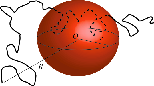
Figure 1: A Brownian particle crossing an interaction sphere. The residence time is the cumulative time spent by the particle inside the sphere.

Very often however, the reaction process is not infinitely efficient, so that the relevant quantity which has to be optimized is not the FPT to the target itself, but rather the residence time of the random walker in the vicinity of the target Agmon (1984). The importance of this observable, defined as the cumulative time spent by the random walker in a given subdomain centered on the target up to a fixed observation time (see figure 1), comes from the fact that it can be seen as a measure of the interaction time between the random walker and the target. The study of the statistics of this general quantity has been a subject of interest for long, both for mathematicians Darling and Kac (1957); Aldous and Fill (1999); Hughes (1995) and physicists Wilemski and Fixman (1973); Agmon (1984); Godrèche and Luck (2001); Majumdar and Comtet (2002); Benichou et al. (2003); Blanco and Fournier (2003); Bénichou et al. (2005); Blanco and Fournier (2006); Grebenkov (2007); Burov and Barkai (2007); Condamin et al. (2007b); Condamin et al. (2008). As a matter of fact, the residence time has proven to be a key quantity in various fields, ranging from astrophysics Ferraro and Zaninetti (2004), transport in porous media Bouchaud and Georges (1990) and diffusion limited reactions Wilemski and Fixman (1973); Agmon (1984); Benichou et al. (2005).

The question we address here is to determine how the residence time depends on transport properties of the random walker, and more precisely on its diffusion coefficient. As we proceed to show, this dependence is non trivial, and in some situations it is possible to tune the value of the diffusion coefficient in order to maximize the residence time.

To get an intuition of this effect, let us start with a simple analysis of the problem. Each time the random walker enters the interaction zone of typical size $r$, it spends inside a typical time of order $r^{2}/D$ which is a decreasing function of the diffusion coefficient $D$. On the other hand, after an observation time $t$, the number of times the interaction zone has been visited is an increasing function of $D$, and behaves like $\sqrt{Dt/r^{2}}$ in dimension 1, $\ln(Dt/r^{2})$ in dimension 2 and like a constant in dimension $d\geq 3$, in the long time limit $t\to\infty$ Hughes (1995). For a walker starting from the exterior of the interaction zone, it is thus clear that both limits of small and large diffusion coefficient $D$ lead to a small residence time, indicating the existence of a maximum as a function of $D$. However, it has to be noted that the observation time has to be finite to make this optimization possible. Indeed, the mean residence time $\mu$ goes to infinity with the observation time in dimension $d\leq 2$, and tends to a constant divided by $D$ in dimension $d\geq 3$, which is a decreasing function of $D$.

With the exception of Bénichou, O. et al. (2008) – which only deals with a one-dimensional situation in the context of DNA/protein interactions – and of Golding and Cox (2006); Guigas and Weiss (2008); Lomholt et al. (2007); Eaves and Reichman (2008); Zaid et al. (2009) – where it has been proposed that slow diffusion could be a way of enhancing the kinetics of imperfect reactions – the dependance of $\mu$ with $D$ does not seem to have received a lot of attention so far, probably for two reasons. First, in most of calculations of residence times, the diffusion coefficient is taken fixed ($D=1/2$ in the mathematical literature, $D=1$ in Berezhkovskii et al. (1998)). Second, the observation time is generally taken to be infinite or at least large in explicit determinations of residence times (see for instance the Section III of Berezhkovskii et al. (1998)), which, as mentioned above, does not permit to reveal the non monotonic behavior we are looking for.

In the following, we focus on the generic case of a Brownian particle evolving in a 3–dimensional space, and discuss three ”experimental” situations, potentially relevant to different problems of chemical reactivity : (i) the observation time is a deterministic variable ; (ii) the observation time is a random variable ; (iii) both the observation time and the starting position of the particle are random.

Denoting ${\bf R}$ the initial position of the particle and $r$ the radius of the target, assumed to be a sphere centered at the origin $O$, we study the pdf $P_{t}(T)$ of the residence time $T$ after an observation time $t$. Following Kac Darling and Kac (1957), we introduce the following trapping problem : we assume that the Brownian particle disappears on the target with a constant and uniform rate $k$. The survival probability $S(t)$ after an observation time $t$ can be written in two different ways. First, it reads

$$S(t)=\int_{0}^{t}P_{t}(t^{\prime})e^{-kt^{\prime}}{\rm d}t^{\prime},$$ (1)

where $e^{-kt^{\prime}}$ represents the survival probability at time $t^{\prime}$ conditioned by the fact that the particle has spent a time $t^{\prime}$ is the reactive zone. Second, it is easy to see that $S$ satisfies the backward Fokker-Planck equation Redner (2001):

$$\partial_{t}S(t)=[D\Delta_{{\bf R}}-kH(r-R)]S(t),$$ (2)

where $H(x)=1$ if $x>0$ and $0$ otherwise, the laplacian $\Delta_{{\bf R}}$ involves derivatives with respect to the starting point ${\bf R}$ and $R\equiv|{\bf R}|$. This partial differential equation has to be completed by the initial condition $S(t)\to 1$ if $t\to 0$ and the boundary condition $S(t)\to 1$ if $R\to\infty$. Denoting by ${\widehat{S}}(s)=\int_{0}^{\infty}e^{-st}S(t){\rm d}t$ the Laplace transform of the survival probability and Laplace transforming Eq. (2), it is easily seen that, if the starting point ${\bf R}$ is exterior to the sphere of radius $r$,

$${\widehat{S}}(s)=\frac{1}{s}+AR^{1-d/2}K_{d/2-1}\left(R\sqrt{\frac{s}{D}}\right),$$ (3)

while if ${\bf R}$ is interior

$${\widehat{S}}(s)=\frac{1}{s+k}+BR^{1-d/2}I_{d/2-1}\left(R\sqrt{\frac{s+k}{D}}\right),$$ (4)

where the constants $A$ and $B$ are given by continuity conditions of the survival probability and of its first spatial derivative at $R=r$, $K_{\nu}$ and $I_{\nu}$ stand for modified Bessel functions and the space dimension is $d$. Note that, in Eqs.(3),(4), only one of the two Bessel functions $I_{d/2-1}$ and $K_{d/2-1}$ generating the set of solutions appears, in order to fulfill boundary conditions when $R\to 0$ and $R\to\infty$. In our case $d=3$, it is explicitly found that, if the starting point is exterior to the sphere of radius $r$,

$${\widehat{S}}(s) = \frac{1}{s}+\frac{e^{-(R-r)\sqrt{s/D}}}{R}\times$$

$$\times \left[\frac{k}{s(s+k)}\frac{\sinh(r\sqrt{(s+k)/D})-r\sqrt{(s+k)/D}\cosh(r\sqrt{(s+k)/D})}{\sqrt{s/D}\sinh(r\sqrt{(s+k)/D})+\sqrt{(s+k)/D}\cosh(r\sqrt{(s+k)/D})}\right],$$

while if it is interior:

$${\widehat{S}}(s) = \frac{1}{s+k}+\frac{\sinh(R\sqrt{(s+k)/D})}{R}\times$$

$$\times \left[\frac{k(1+r\sqrt{s/D})}{p(p+k)}\frac{1}{\sqrt{s/D}\sinh(r\sqrt{(s+k)/D})+\sqrt{(s+k)/D}\cosh(r\sqrt{(s+k)/D})}\right].$$

The Laplace transform ${\widehat{\mu}}(s)$ of the mean residence time $\mu(t)$ is then obtained by expanding Eqs(Optimization of the residence time of a Brownian particle in a spherical subdomain)-(Optimization of the residence time of a Brownian particle in a spherical subdomain) as a function of the parameter $k$, since ${\widehat{S}}(s)$ writes:

$${\widehat{S}}(s) = \int_{0}^{\infty}{\rm d}te^{-st}\int_{0}^{t}{\rm d}t^{\prime}e^{-kt^{\prime}}P_{t}(t^{\prime})=\frac{1}{s}-k{\widehat{\mu}}(s)+o(k)$$ (7)

If the starting point is exterior to the sphere of radius $r$, the small $k$ expansion of Eq(Optimization of the residence time of a Brownian particle in a spherical subdomain) leads to :

$${\widehat{\mu}}(s)=\frac{1}{s^{2}}\frac{e^{-R\sqrt{s/D}}}{R\sqrt{s/D}}[{r\sqrt{s/D}\cosh(r\sqrt{s/D})-\sinh(r\sqrt{s/D})}],$$ (8)

while if the starting point is interior to the sphere of radius $r$, the small $k$ expansion of Eq(Optimization of the residence time of a Brownian particle in a spherical subdomain) leads to :

$${\widehat{\mu}}(s)=\frac{1}{s^{2}}\left(1-\frac{(1+r\sqrt{s/D})\sinh({R\sqrt{s/D}})}{R\sqrt{s/D}\exp(r\sqrt{s/D})}\right),$$ (9)

Deterministic observation time. In the first case of a deterministic observation time $t$, corresponding for instance to a chemical reaction designed to be terminated after a time $t$, it is actually possible to Laplace invert the transform of the mean residence time. Using the two known Laplace inverts:

$${\cal L}^{-1}(e^{-\sqrt{s}}/s^{2})(t)=-\sqrt{{\frac{t}{\pi}}}{{\rm e}^{-1/(4\,{t})}}+\frac{1}{2}\,\left(1-{\rm erf}\left({\frac{1}{2\sqrt{t}}}\right)\right)\left(2\,t+1\right)$$ (10)

$${\cal L}^{-1}(e^{-\sqrt{s}}/s^{5/2})(t)=-\frac{1}{6}\,\left(1-{\rm erf}\left({\frac{1}{2\sqrt{t}}}\right)\right)\left(1+6\,t\right)+\frac{1}{3}\,\sqrt{{\frac{t}{\pi}}}{{\rm e}^{-1/(4\,{t})}}\left(4\,t+1\right)$$ (11)

where ${\cal L}^{-1}$ stands for the inverse Laplace operator and ${\rm erf}(x)$ is the error function, a direct Laplace inversion of Eqs.(8),(9) gives the explicit expression

$$\mu(t)=\phi(r,R;t)-\phi(-r,R;t)+\left\{\begin{array}[]{lll}\displaystyle\frac{1}{2D}(r^{2}-R^{2}/3),\;\;\;{R<r},\\ \\ \displaystyle\frac{r^{3}}{3RD},\;\;\;{R>r},\end{array}\right.$$

where

$$\phi(r,R;t)=\frac{2}{3}\sqrt{\frac{D}{\pi}}\frac{t^{3/2}}{R}\left(1+\frac{(R+r)(R-2r)}{4Dt}\right)e^{-\frac{(R+r)^{2}}{4Dt}}$$

$$+\frac{1}{2}{\rm erf}\left(\frac{r+R}{2\sqrt{Dt}}\right)\left(t+\frac{R^{2}}{6D}-\frac{r^{3}}{3DR}-\frac{r^{2}}{2D}\right).$$ (12)

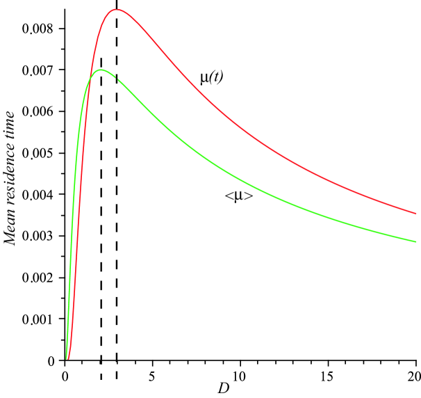
Figure 2: The mean residence time as a function of the diffusion coefficient for deterministic ($t=1$) and random observation times ($p=1$). In both cases, the Brownian particle starts outside of the sphere ($R=3$, $r=1$). The optimal diffusion coefficient in the deterministic case (resp. random) is well approximated by the limiting expression $D_{0}\approx\alpha R^{2}/t$ (resp. $D_{0}\approx pR^{2}/4$) given in the text, even if here the condition of applicability $R\gg r$ is not well satisfied.

Note that in the limit of large observation times $t\to\infty$, this expression gives back the known results of Berezhkovskii et al. (1998) : $\displaystyle\mu(\infty)=\frac{3r^{2}-R^{2}}{6D}$ if $R<r$ (compare with Eq.(3.16a) of Berezhkovskii et al. (1998)) and $\displaystyle\mu(\infty)=\frac{r^{3}}{3RD}$ if $R>r$ (compare with Eq.(3.11) of Berezhkovskii et al. (1998)). Moreover, as expected, it is easily seen that, if $R>r$, $\mu(t)\to 0$ if $D\to 0$ or if $D\to\infty$. As a consequence, there exists a value of $D_{0}$ that optimizes the residence time (see figure 2). Deriving the expressions of $\mu(t)$ with respect to $D$, this optimal value is easily seen to satisfy the following implicit equation:

$$-2\,{{\rm e}^{-{\frac{\left(R+r\right)^{2}}{4D_{0}t}}}}\sqrt{D_{0}t}\left({R}^{2}-2\,{r}^{2}-Rr-2\,D_{0}t\right)+2\,{{\rm e}^{-{\frac{\left(-r+R\right)^{2}}{4D_{0}t}}}}\sqrt{D_{0}t}\left({R}^{2}+Rr-2\,D_{0}t-2\,{r}^{2}\right)$$

$$-\sqrt{\pi}{{\rm erf}\left({\frac{R+r}{2\sqrt{D_{0}t}}}\right)}\left(R-2\,r\right)\left(R+r\right)^{2}+\sqrt{\pi}{{\rm erf}\left({\frac{-r+R}{2\sqrt{D_{0}t}}}\right)}\left(2\,r+R\right)\left(-r+R\right)^{2}=0$$ (13)

whose solution can be discussed in limiting regimes. When $R\gg r$, we find that $D_{0}\sim\alpha R^{2}/t$, where $\alpha\simeq 0.353$ is the implicit solution of the equation

$$2\sqrt{\pi}\left[{\rm erf}\left(\frac{1}{2\sqrt{\alpha}}\right)-1\right]+\frac{e^{-1/(4\alpha)}}{\sqrt{\alpha}}=0,$$ (14)

obtained by replacing $D_{0}$ by $\alpha R^{2}/t$ in Eq.(Optimization of the residence time of a Brownian particle in a spherical subdomain) and taking the limit $R\gg r$. In other words, the optimal diffusion coefficient $D_{0}$ does not depend of the extension of the target $r$ in this regime. This is in strong contrast with the opposite regime $R\to r^{+}$, which leads after a similar analysis to an optimal diffusion coefficient $D_{0}\sim 3r^{2}(R/r-1)/(2t)$, which, in particular, vanishes when $R\to r^{+}$ as could be expected from the qualitative analysis presented above.

Random observation time. We now consider another experimental situation, corresponding to a random observation time, distributed according to an exponential law with mean $1/p$. This case corresponds for example to a situation where the particle has a finite lifetime, as in many biological situations. Averaging over this random lifetime, the mean residence time becomes:

$$\langle\mu\rangle\equiv\int_{0}^{\infty}{\rm d}tpe^{-pt}\int_{0}^{t}{\rm d}t^{\prime}t^{\prime}P_{t}(t^{\prime})\equiv p{\widehat{\mu}}(s=p),$$ (15)

where ${\widehat{\mu}}(s)$ is given by Eqs.(9)-(8). Once again, for $R>r$, the mean residence time can be shown to have an optimum as a function of $D$ (see figure 2). Interestingly, the optimal diffusion coefficient $D_{0}$ satisfies the simple implicit equation

$$\tanh{x}=\frac{ax^{2}+x}{x^{2}+ax+1},$$ (16)

where $x=r\sqrt{p/D_{0}}$ and $a=R/r$.

For $a\gg 1$ , the Lagrange inversion formula Wilf (1990) allows one to obtain explicitly the expansion of $x$ as powers of $1/a$, up to arbitrary order. The first terms are given by: $x=\frac{2}{a}+\frac{4}{5a^{3}}+...$. In the opposite limit $a\to 1$, it is easy to deduce from Eq. (16) that $\displaystyle x\sim\frac{1}{\sqrt{a-1}}$. Finally, this gives again two regimes for the optimal diffusion coefficient: $D_{0}\sim pR^{2}/4$ when $R\gg r$ and $D_{0}\sim pr^{2}(R/r-1)$ when $R\to r^{+}$, in close analogy with the two regimes found in the case of a deterministic observation time.

Random observation time and random initial position. In the last situation, we assume that both the observation time and the initial position are random variables. More precisely, the observation time is again assumed to be distributed according to an exponential law with mean $1/p$, while the initial position is assumed to be uniformly distributed in an annulus region centered on 0, of inner radius $b$ and outer radius $c$. This mimics for example a case of chemical reactions where the position of the source of reactants cannot be accurately determined. In this case of an annulus region, it is not clear a priori if the mean residence time is still non trivially optimizable with respect to $D$. Indeed, if the initial position is within the reactive sphere, the best diffusion coefficient is simply $D_{0}=0$. On the contrary, if the annulus region is entirely exterior to the reactive sphere, a non trivial optimal $D_{0}$ is expected from previous results. This raises the question of the intermediate case where the annulus partially covers the reactive sphere.

In the first case of an annulus region exterior to the target zone ($b>r$), we find

$$\overline{\langle\mu\rangle}=\frac{3rl}{p(c^{3}-b^{3})}\left[\frac{\sinh(r/l)}{r/l}-\cosh(r/l)\right]$$ (17)

$$\times \left[\left(c+l\right)e^{-c/l}-\left(b+l\right)e^{-b/l}\right],$$

where $l\equiv\sqrt{D/p}$. This quantity is easily shown to tend towards 0 when $D\to\infty$ while

$$\overline{\langle\mu\rangle}\sim_{D\to 0}\frac{3rbl}{2p(c^{3}-b^{3})}e^{-(b-r)/l}>0.$$ (18)

This proves that $\overline{\langle\mu\rangle}$ admits an optimum diffusion coefficient, as expected in view of the previous results.

In the opposite situation of a annulus region such that $0<b<r<c$, we get

$$\overline{\langle\mu\rangle}-\frac{1}{p}\frac{r^{3}-b^{3}}{c^{3}-b^{3}}=\frac{3l}{p(c^{3}-b^{3})}\times$$

$$\left[e^{-r/l}\left(r+l\right)\left(b\cosh\left(b/l\right)-l\sinh\left(b/l\right)\right)\right.$$

$$\left.-e^{-c/l}\left(c+l\right)\left(r\cosh\left(r/l\right)-l\sinh\left(r/l\right)\right)\right].$$ (19)

The local behavior of this quantity when $D\to 0$ actually depends on the relative order of the two distances $r-b$ and $c-r$. If $r-b<c-r$,

$$\overline{\langle\mu\rangle}-\frac{1}{p}\frac{r^{3}-b^{3}}{c^{3}-b^{3}}\sim\frac{3rbl}{2p(c^{3}-b^{3})}e^{-(r-b)/l}>0,$$ (20)

showing that there is an optimal diffusion coefficient.

Remarkably, if $r-b>c-r$,

$$\overline{\langle\mu\rangle}-\frac{1}{p}\frac{r^{3}-b^{3}}{c^{3}-b^{3}}\sim-\frac{3}{p(c^{3}-b^{3})}\sqrt{\frac{D}{p}}\frac{rc}{2}e^{-(c-r)\sqrt{p/D}}<0,$$ (21)

and this time there is no possible optimization.

The last case of an annulus region of inner radius equal to zero (i.e. $b=0$), i.e. a sphere of radius $c$, deserves some specific attention. In this case, Eq. (Optimization of the residence time of a Brownian particle in a spherical subdomain) is still valid but, quite surprisingly, no optimization with respect to the diffusion coefficient is possible. This monotonic decrease is compatible with the local behavior ($D\to 0$):

$$\overline{\langle\mu\rangle}-\frac{1}{p}\frac{r^{3}}{c^{3}}\sim-\frac{3r}{2pc^{2}}\sqrt{\frac{D}{p}}e^{-(c-r)\sqrt{p/D}}<0.$$ (22)

We stress that this result holds for arbitrary values of the radius $c$.

In conclusion, we have proposed a very simple mechanism that allows one to optimize the residence time of diffusing molecules with respect to the diffusion coefficient. We have discussed the relevance of this effect to several schematic experimental situations, classified in the nature – random or deterministic – both of the observation time and of the starting position. We believe that this optimization of the residence time discussed in the case of the standard Brownian motion is robust (see in particular Supplementary Material for a discussion of a discrete space version of the model presented here) and is generalizable to more complex transport processes.

Figure captions:

Fig1: A Brownian particle crossing an interaction sphere. The residence time is the cumulative time spent by the particle inside the sphere.

Fig2: The mean residence time as a function of the diffusion coefficient for deterministic ($t=1$) and random observation times ($p=1$). In both cases, the Brownian particle starts outside of the sphere ($R=3$, $r=1$). The optimal diffusion coefficient in the deterministic case (resp. random) is well approximated by the limiting expression $D_{0}\approx\alpha R^{2}/t$ (resp. $D_{0}\approx pR^{2}/4$) given in the text, even if here the condition of applicability $R\gg r$ is not well satisfied.

References

- van Kampen (1992) N. G. van Kampen, Stochastic Processes in Physics and Chemistry (North-Holland, Amsterdam, 1992).
- Redner (2001) S. Redner, A guide to First- Passage Processes (Cambridge University Press, 2001).
- Condamin et al. (2005) S. Condamin, O. Bénichou, and M. Moreau, Phys Rev Lett 95, 260601 (2005); Phys Rev E 72, 016127 (2005).
- Condamin et al. (2007a) S. Condamin, O. Bénichou, V. Tejedor, R. Voituriez, and J. Klafter, Nature 450, 77 (2007a); O. Bénichou and R. Voituriez, Phys Rev Lett 100, 168105 (2008a); O. Bénichou, B. Meyer V. Tejedor, and R. Voituriez, Phys Rev Lett 101, 130601 (2008a)
- (5) O. Bénichou, C. Loverdo, M. Moreau, and R. Voituriez, Physical Chemistry Chemical Physics 10, 7059 (2008).
- Rice (1985) S. Rice, Diffusion-Limited Reactions (Elsevier, Amsterdam, 1985).
- S.B.Yuste and K.Lindenberg (2002) S.B.Yuste and K.Lindenberg, Chem.Phys. 284, 169 (2002).
- Benichou et al. (2005) O. Bénichou, M. Coppey, M. Moreau, P.-H. Suet, and R. Voituriez, Phys Rev Lett 94, 198101 (2005); J. Phys.: Condens. Matter 17, S4275 (2005).
- Benichou et al. (2006) O. Bénichou, C. Loverdo, M. Moreau, and R. Voituriez, Phys Rev E 74, 020102 (2006); J. Phys.: Condens. Matter 19, 065141 (2007).
- Darling and Kac (1957) D. A. Darling and M. Kac, Trans. Am. Math. Soc. 84, 444 (1957).
- Aldous and Fill (1999) D. Aldous and J. Fill, Reversible Markov chains and random walks on graphs (http://www.stat.berkeley.edu /users/aldous/RWG/book.html, 1999).
- Hughes (1995) B. D. Hughes, Random Walks and Random Environments (Oxford Press, 1995).
- Wilemski and Fixman (1973) G. Wilemski and M. Fixman, J. Chem. Phys. 58, 4009 (1973).
- Agmon (1984) N. Agmon, J. Chem. Phys. 81, 3644 (1984).
- Godrèche and Luck (2001) C. Godrèche and J. Luck, J. Stat. Phys. 104, 489 (2001).
- Majumdar and Comtet (2002) S. Majumdar and A. Comtet, Phys. Rev. Lett. 89, 60601 (2002).
- Benichou et al. (2003) O. Bénichou, M. Coppey, J. Klafter, M. Moreau, and G. Oshanin, J. Phys. A 36, 7225 (2003); J. Phys. A 38, 7205 (2003).
- Blanco and Fournier (2003) S. Blanco and R. Fournier, EPL 61, 168 (2003).
- Bénichou et al. (2005) O. Bénichou, M. Coppey, M. Moreau, P. H. Suet, and R. Voituriez, EPL 70, 42 (2005).
- Blanco and Fournier (2006) S. Blanco and R. Fournier, Phys. Rev. Lett. 97, 230604 (2006).
- Grebenkov (2007) D. S. Grebenkov, Phys Rev E 76, 041139 (2007).
- Burov and Barkai (2007) S. Burov and E. Barkai, Phys Rev Lett 98, 250601 (2007).
- Condamin et al. (2007b) S. Condamin, V. Tejedor, and O. Bénichou, Phys Rev E 76, 050102 (2007b).
- Condamin et al. (2008) S. Condamin, V. Tejedor, R. Voituriez, O. Bénichou, and J. Klafter, PNAS 105, 5675 (2008).
- Ferraro and Zaninetti (2004) M. Ferraro and L. Zaninetti, Physica A 338, 307 (2004).
- Bouchaud and Georges (1990) J.-P. Bouchaud and A. Georges, Physics Reports 195, 127 (1990).
- Benichou et al. (2005) O. Benichou, M. Coppey, M. Moreau, and G. Oshanin, J Chem Phys 123, 194506 (2005).
- Bénichou, O. et al. (2008) Bénichou, O. , Loverdo, C. , and Voituriez, R. , EPL 84, 38003 (2008).
- Golding and Cox (2006) E. Golding and E. Cox, Phys. Rev. Lett. 96, 981102 (2006).
- Guigas and Weiss (2008) G. Guigas and M. Weiss, Biophys. J. 94, 90 (2008).
- Lomholt et al. (2007) M. A. Lomholt, I. M. Zaid, and R. Metzler, Physical Review Letters 98, 200603 (2007).
- Eaves and Reichman (2008) J. D. Eaves and D. R. Reichman, The Journal of Physical Chemistry B 112, 4283 (2008).
- Zaid et al. (2009) I. M. Zaid, M. A. Lomholt, and R. Metzler, 97, 710 (2009).
- Berezhkovskii et al. (1998) A. M. Berezhkovskii, V. Zaloj, and N. Agmon, Physical Review E 57, 3937 (1998).
- Wilf (1990) H. S. Wilf, Generating functionalogy (Academic Press, New York, 1990).