Minimax Manifold Estimation

Abstract

We find the minimax rate of convergence in Hausdorff distance for estimating a manifold $M$ of dimension $d$ embedded in $\mathbb{R}^{D}$ given a noisy sample from the manifold. Under certain conditions, we show that the optimal rate of convergence is $n^{-2/(2+d)}$. Thus, the minimax rate depends only on the dimension of the manifold, not on the dimension of the space in which $M$ is embedded.

Keywords: Manifold learning, Minimax estimation.

1 Introduction

We consider the problem of estimating a manifold $M$ given noisy observations near the manifold. The observed data are a random sample $Y_{1},\ldots,Y_{n}$ where $Y_{i}\in\mathbb{R}^{D}$. The model for the data is

$$Y_{i}=\xi_{i}+Z_{i}$$ (1)

where $\xi_{1},\ldots,\xi_{n}$ are unobserved variables drawn from a distribution supported on a manifold $M$ with dimension $d<D$. The noise variables $Z_{1},\ldots,Z_{n}$ are drawn from a distribution $F$. Our main assumption is that $M$ is a compact, $d$-dimensional, smooth Riemannian submanifold in $\mathbb{R}^{D}$; the precise conditions on $M$ are given in Section 2.1.

A manifold $M$ and a distribution for $(\xi,Z)$ induce a distribution $Q\equiv Q_{M}$ for $Y$. In Section 2.2, we define a class of such distributions

$${\cal Q}=\Bigl{\{}Q_{M}:\ M\in{\cal M}\Bigr{\}}$$ (2)

where ${\cal M}$ is a set of manifolds. Given two sets $A$ and $B$, the Hausdorff distance between $A$ and $B$ is

$$H(A,B)=\inf\Bigl{\{}\epsilon:\ A\subset B\oplus\epsilon\ \ \ {\rm and}\ \ \ \ B\subset A\oplus\epsilon\Bigr{\}}$$ (3)

where

$$A\oplus\epsilon=\bigcup_{x\in A}B_{D}(x,\epsilon)$$ (4)

and $B_{D}(x,\epsilon)$ is an open ball in $\mathbb{R}^{D}$ centered at $x$ with radius $\epsilon$. We are interested in the minimax risk

$$R_{n}({\cal Q})=\inf_{\widehat{M}}\sup_{Q\in{\cal Q}}\mathbb{E}_{Q}[H(\widehat{M},M)]$$ (5)

where the infimum is over all estimators $\widehat{M}$. By an estimator $\widehat{M}$ we mean a measurable function of $Y_{1},\ldots,Y_{n}$ taking values in the set of all manifolds. Our first main result is the following minimax lower bound which is proved in Section 3.

Theorem 1

Under the conditions given in Section 2, there is a constant $C_{1}>0$ such that, for all large $n$,

$$\inf_{\widehat{M}}\sup_{Q\in{\cal Q}}\mathbb{E}_{Q}\left[H(\widehat{M},M)\right]\geq C_{1}\,\left(\frac{1}{n}\right)^{\frac{2}{2+d}}$$ (6)

where the infimum is over all estimators $\widehat{M}$.

Thus, no method of estimating $M$ can have an expected Hausdorff distance smaller than the stated bound. Note that the rate depends on $d$ but not on $D$ even though the support of the distribution $Q$ for $Y$ has dimension $D$. Our second result is the following upper bound which is proved in Section 4.

Theorem 2

Under the conditions given in Section 2, there exists an estimator $\widehat{M}$ such that, for all large $n$,

$$\sup_{Q\in{\cal Q}}\mathbb{E}_{Q}\left[H(\widehat{M},M)\right]\leq C_{2}\,\left(\frac{\log n}{n}\right)^{\frac{2}{2+d}}$$ (7)

for some $C_{2}>0$.

Thus the rate is tight, up to logarithmic factors. The estimator in Theorem 2 is of theoretical interest because it establishes that the lower bound is tight. But, the estimator constructed in the proof of that theorem is not practical and so in Section 5, we construct a very simple estimator $\widehat{M}$ such that

$$\sup_{Q\in{\cal Q}}\mathbb{E}_{Q}\left[H(\widehat{M},M)\right]\leq\left(\frac{C\log n}{n}\right)^{1/D}.$$ (8)

This is slower than the minimax rate, but the estimator is computationally very simple and requires no knowledge of $d$ or the smoothness of $M$.

Related Work. There is a vast literature on manifold estimation. Much of the literature deals with using manifolds for the purpose of dimension reduction. See, for example, Baraniuk and Wakin (2007) and references therein. We are interested instead in actually estimating the manifold itself. There is a large literature on this problem in the field of computational geometry; see, for example, Dey (2006), Dey and Goswami (2004), Chazal and Lieutier (2008) Cheng and Dey (2005) and Boissonnat and Ghosh (2010). However, very few papers allow for noise in the statistical sense, by which we mean observations drawn randomly from a distribution. In the literature on computational geometry, observations are called noisy if they depart from the underlying manifold in a very specific way: the observations have to be close to the manifold but not too close to each other. This notion of noise is quite different from random sampling from a distribution. An exception is Niyogi et al. (2008) who constructed the following estimator. Let $I=\{i:\ \widehat{p}(Y_{i})>\lambda\}$ where $\widehat{p}$ is a density estimator. They define $\widehat{M}=\bigcup_{i\in I}B_{D}(Y_{i},\epsilon)$ and they show that if $\lambda$ and $\epsilon$ are chosen properly, then $\widehat{M}$ is homologous to $M$. (This means that $M$ and $\widehat{M}$ share certain topological properties.) However, the result does not guarantee closeness in Hausdorff distance. Note that $\bigcup_{i=1}^{n}B_{D}(Y_{i},\epsilon)$ is precisely the Devroye-Wise estimator for the support of a distribution (Devroye and Wise (1980)).

Notation. Given a set $S$, we denote its boundary by $\partial S$. We let $B_{D}(x,r)$ denote a $D$-dimensional open ball centered at $x$ with radius $r$. If $A$ is a set and $x$ is a point then we write $d(x,A)=\inf_{y\in A}||x-y||$ where $||\,\cdot\,||$ is the Euclidean norm. Let

$$A\circ B=(A\cap B^{c})\,\bigcup\,(A^{c}\cap B)$$ (9)

denote symmetric set difference between sets $A$ and $B$.

The uniform measure on a manifold $M$ is denoted by $\mu_{M}$. Lebesgue measure on $\mathbb{R}^{k}$ is denoted by $\nu_{k}$. In case $k=D$, we sometimes write $V$ instead of $\nu_{D}$; in other words $V(A)$ is simply the volume of $A$. Any integral of the form $\int f$ is understood to be the integral with respect to Lebesgue measure on $\mathbb{R}^{D}$. If $P$ and $Q$ are two probability measures on $\mathbb{R}^{D}$ with densities $p$ and $q$ then the Hellinger distance between $P$ and $Q$ is

$$h(P,Q)\equiv h(p,q)=\sqrt{\int(\sqrt{p}-\sqrt{q})^{2}}=\sqrt{2\left(1-\int\sqrt{pq}\right)}$$ (10)

where the integrals are with respect to $\nu_{D}$. Recall that

$$\ell_{1}(p,q)\leq h(p,q)\leq\sqrt{\ell_{1}(p,q)}$$ (11)

where $\ell_{1}(p,q)=\int|p-q|$. Let $p(x)\wedge q(x)=\min\{p(x),q(x)\}$. The affinity between $P$ and $Q$ is

$$||P\wedge Q||=\int p\wedge q=1-\frac{1}{2}\int|p-q|.$$ (12)

Let $P^{n}$ denote the $n$-fold product measure based on $n$ independent observations from $P$. In the appendix Section 7.1 we show that

$$||P^{n}\wedge Q^{n}||\geq\frac{1}{8}\left(1-\frac{1}{2}\int|p-q|\right)^{2n}.$$ (13)

We write $X_{n}=O_{P}(a_{n})$ to mean that, for every $\epsilon>0$ there exists $C>0$ such that $\mathbb{P}(||X_{n}||/a_{n}>C)\leq\epsilon$ for all large $n$. Throughout, we use symbols like $C,C_{0},C_{1},c,c_{0},c_{1}\ldots$ to denote generic positive contants whose value may be different in different expressions.

2 Model Assumptions

2.1 Manifold Conditions

We shall be concerned with $d$-dimensional compact Riemannian submanifolds without boundary embedded in $\mathbb{R}^{D}$ with $d<D$. (Informally, this means that $M$ looks like $\mathbb{R}^{d}$ in a small neighborhood around any point in $M$.) We assume that $M$ is contained in some compact set ${\cal K}\subset\mathbb{R}^{D}$.

At each $u\in M$ let $T_{u}M$ denote the tangent space to $M$ and let $T_{u}^{\perp}M$ be the normal space. We can regard $T_{u}M$ as a $d$-dimensional hyperplane in $\mathbb{R}^{D}$ and we can regard $T_{u}^{\perp}M$ as the $D-d$ dimensional hyperplane perpendicular to $T_{u}M$. Define the fiber of size $a$ at $u$ to be $L_{a}(u)\equiv L_{a}(u,M)=T_{u}^{\perp}M\bigcap B_{D}(u,a)$.

Let $\Delta(M)$ be the largest $r$ such that each point in $M\oplus r$ has a unique projection onto $M$. The quantity $\Delta(M)$ will be small if either $M$ highly curved or if $M$ is close to being self-intersecting. Let ${\cal M}\equiv{\cal M}(\kappa)$ denote all $d$-dimensional manifolds embedded in ${\cal K}$ such that $\Delta(M)\geq\kappa$. Throughout this paper, $\kappa$ is a fixed positive constant. The quantity $\Delta(M)$ has been rediscovered many times. It is called the condition number in Niyogi et al. (2006), the thickness in Gonzalez and Maddocks (1999) and the reach in Federer (1959).

An equivalent definition of $\Delta(M)$ is the following: $\Delta(M)$ is the largest number $r$ such that the fibers $L_{r}(u)$ never intersect. See Figure 1. Note that if $M$ is a sphere then $\Delta(M)$ is just the radius of the sphere and if $M$ is a linear space then $\Delta(M)=\infty$. Also, if $\sigma<\Delta(M)$ then $M\oplus\sigma$ is the disjoint union of its fibers:

$$M\oplus\sigma=\bigcup_{u\in M}L_{\sigma}(u).$$ (14)

Define ${\sf tube}(M,a)=\bigcup_{u\in M}L_{a}(u).$ Thus, if $\sigma<\Delta(M)$ then $M\oplus\sigma={\sf tube}(M,\sigma)$.

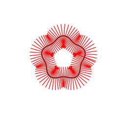
Figure 1: The condition number $\Delta(M)$ of a manifold is the largest number $\kappa$ such that the normals to the manifold do not cross as long as they are not extended beyond $\kappa$. The plot on the left shows a one-dimensional manifold (a curve) and some normals of length $r<\kappa$. The plot on the right shows the same manifold and some normals of length $r>\kappa$.

Let $p,q\in M$. The angle between two tangent spaces $T_{p}$ and $T_{q}$ is defined to be

$${\sf angle}(T_{p},T_{q})=\cos^{-1}\Bigl{(}\min_{u\in T_{p}}\max_{v\in T_{q}}|\langle u-p,v-q\rangle|\Bigr{)}$$ (15)

where $\langle u,v\rangle$ is the usual inner product in $\mathbb{R}^{D}$. Let $d_{M}(p,q)$ denote the geodesic distance between $p,q\in M$.

We now summarize some useful results from Niyogi et al. (2006).

Lemma 3

Let $M\subset{\cal K}$ be a manifold and suppose that $\Delta(M)=\kappa>0$. Let $p,q\in M$.

1. Let $\gamma$ be a geodesic connecting $p$ and $q$ with unit speed parameterization. Then the curvature of $\gamma$ is bounded above by $1/\kappa$.

2. $\cos(\mathop{\sf angle}(T_{p},T_{q}))>1-d_{M}(p,q)/\kappa$. Thus, $\mathop{\sf angle}(T_{p},T_{q})\leq\sqrt{2d_{M}(p,q)/\kappa}+o(\sqrt{d_{M}(p,q)/\kappa})$.

3. If $a=||p-q||\leq\kappa/2$ then $d_{M}(p,q)\leq\kappa-\kappa\sqrt{1-(2a)/\kappa}=a+o(a)$.

4. If $a=||p-q||\leq\kappa/2$ then $a\geq d_{M}(p,q)-(d_{M}(p,q))^{2}/(2\kappa)$.

5. If $||q-p||>\epsilon$ and $v\in B_{D}(q,\epsilon)\cap T_{p}^{\perp}M\cap B_{D}(p,\kappa)$ then $||v-p||<\epsilon^{2}/\kappa$.

6. Fix any $\delta>0$. There exists points $x_{1},\ldots,x_{N}\in M$ such that $M\subset\bigcup_{j=1}^{N}B_{D}(x_{j},\delta)$ and such that $N\leq(c/\delta)^{d}$.

For further information about manifolds, see Lee (2002).

2.2 Distributional Assumptions

The distribution of $Y$ is induced by the distribution of $\xi$ and $Z$. We will assume that $\xi$ is drawn uniformly on the manifold. Then we assume that $Z$ is drawn uniformly on the normal to $M$. More precisely, given $\xi$, we draw $Z$ uniformly on $L_{\sigma}(\xi)$. In other words, the noise is perpendicular to the manifold. The result is that, if $\sigma<\kappa$, then the distribution $Q=Q_{M}$ of $Y$ has support equal to $M\oplus\sigma$.

The distributional assumption on $\xi$ is not critical. Any smooth density bounded away from 0 on the manifold will lead to similar results. However, the assumption on the noise $Z$ is critical. We have chosen the simplest noise distribution here. (Perpendicular noise is also assumed in Niyogi et al. (2008).) In current work, we are deriving the rates for more complicated noise distributions. The rates are quite different and the proofs are more complex. Those results will be reported elsewhere.

The set of distributions we consider is as follows. Let $\kappa$ and $\sigma$ be fixed positive numbers such that $0<\sigma<\kappa$. Let

$${\cal Q}\equiv{\cal Q}(\kappa,\sigma)=\Bigl{\{}Q_{M}:\ M\in{\cal M}(\kappa)\Bigr{\}}.$$ (16)

For any $M\in{\cal M}(\kappa)$ consider the corresponding distribution $Q_{M}$, supported on $S_{M}=M\oplus\sigma$. Let $q_{M}$ be the density of $Q_{M}$ with respect to Lebesgue measure. We now show that $q_{M}$ is bounded above and below by a uniform density.

Recall that the essential supremum and essential infimum of $q_{M}$ are defined by

$$\operatorname*{ess\,sup}_{y\in A}q_{M}=\inf\Bigl{\{}a\in\mathbb{R}:\ \nu_{D}(\{y:\ q_{M}(y)>a\}\cap A)=0\Bigr{\}}$$

and

$$\operatorname*{ess\,inf}_{y\in A}q_{M}=\sup\Bigl{\{}a\in\mathbb{R}:\ \nu_{D}(\{y:\ q_{M}(y)<a\}\cap A)=0\Bigr{\}}.$$

Also recall that, by the Lebesgue density theorem, $q_{M}(y)=\lim_{\epsilon\to 0}Q_{M}(B_{D}(y,\epsilon))/V(B_{D}(y,\epsilon))$ for almost all $y$. Let $U_{M}$ be the uniform distribution on $M\oplus\sigma$ and let $u_{M}=1/V(M\oplus\sigma)$ be the density of $U_{M}$. Note that, for $A\subset M\oplus\sigma$, $U_{M}(A)=V(A)/V(M\oplus\sigma)$.

Lemma 4

There exist constants $0<C_{*}\leq C^{*}<\infty$, depending only on $\kappa$ and $d$, such that

$$C_{*}\leq\inf_{M\in{\cal M}}\operatorname*{ess\,inf}_{y\in S_{M}}\frac{q_{M}(y)}{u_{M}(y)}\leq\sup_{M\in{\cal M}}\operatorname*{ess\,sup}_{y\in S_{M}}\frac{q_{M}(y)}{u_{M}(y)}\leq C^{*}.$$ (17)

Proof  Choose any $M\in{\cal M}(\kappa)$. Let $x$ by any point in the interior of $S_{M}$. Let $B=B_{D}(x,\epsilon)$ where $\epsilon>0$ is small enough so that $B\subset S_{M}=M\oplus\sigma$. Let $y$ be the projection of $x$ onto $M$. We want to upper and lower bound $Q(B)/V(B)$. Then we will take the limit as $\epsilon\to 0$. Consider the two spheres of radius $\kappa$ tangent to $M$ at $y$ in the direction of the line between $x$ and $y$. (See Figure 2.) Note that $Q(B)$ is maximized by taking $M$ to be equal to the upper sphere and $Q(B)$ is minimized by taking $M$ to be equal to the lower sphere. Let us consider first the case where $M$ is equal to the upper sphere. Let

$$U=\Bigl{\{}u\in M:\ L_{\sigma}(u)\cap B\neq\emptyset\Bigr{\}}$$

be the projection of $B$ onto $M$. By simple geometry, $U=M\cap B_{D}(y,r\epsilon)$ where

$$\left(1+\frac{\sigma}{\kappa}\right)^{-1}\leq r\leq\left(1+\frac{\sigma}{\kappa}\right).$$

Let ${\sf Vol}$ denote $d$-dimensional volume on $M$. Then ${\sf Vol}(B_{D}(y,r\epsilon)\cap M)\leq c_{1}r^{d}\epsilon^{d}\omega_{d}$ where $\omega_{d}$ is the volume of a unit $d$-ball and $c_{1}$ depends only on $\kappa$ and $d$. To see this, note that because $M$ is a manifold and $\Delta(M)\geq\kappa$, it follows that near $y$, $M$ may be locally parameterized as a smooth function $f=(f_{1},\ldots,f_{D-d})$ over $B\cap T_{y}M$. The surface area of the graph of $f$ over $B\cap T_{y}M$ is bounded by $\int_{B_{D}(y,r\epsilon)\cap T_{y}M}\sqrt{1+\left\|\nabla f_{i}\right\|^{2}}$, which is bounded by a constant $c_{1}$ uniformly over ${\cal M}$. Hence, ${\sf Vol}(B_{D}(y,r\epsilon)\cap M)\leq c_{1}{\sf Vol}(B_{D}(y,r\epsilon)\cap T_{y}M)=c_{1}r^{d}\epsilon^{d}\omega_{d}$.

Let $\Lambda_{M}$ be the uniform distribution on $M$ and let $\Gamma_{u}$ denote the uniform measure on $L_{\sigma}(u)$. Note that, for $u\in U$, $L_{\sigma}(u)\cap B$ is a $(D-d)$-ball whose radius is at most $\epsilon$. Hence,

$$\Gamma_{u}(L_{\sigma}(u)\cap B)\leq\frac{\epsilon^{D-d}\omega_{D-d}}{\sigma^{D-d}\omega_{D-d}}=\left(\frac{\epsilon}{\sigma}\right)^{D-d}.$$

Thus,

$$Q_{M}(B) = \int_{M}\Gamma_{u}(B\cap L_{\sigma}(u))d\Lambda_{M}(u)=\int_{U}\Gamma_{u}(B\cap L_{\sigma}(u))d\Lambda_{M}(u)$$

$$\leq \left(\frac{\epsilon}{\sigma}\right)^{D-d}\Lambda(U)=\left(\frac{\epsilon}{\sigma}\right)^{D-d}\frac{{\sf Vol}(B_{D}(y,r)\cap M)}{{\sf Vol}(M)}$$

$$\leq \left(\frac{\epsilon}{\sigma}\right)^{D-d}\frac{\epsilon^{d}r^{d}\omega_{d}}{{\sf Vol}(M)}\leq\left(\frac{\epsilon}{\sigma}\right)^{D-d}\frac{\epsilon^{d}(1+\sigma/\kappa)^{d}\omega_{d}}{{\sf Vol}(M)}.$$

Now, $U_{M}(B)=V(B)/V(M\oplus\sigma)=\epsilon^{D}\omega_{D}/(\sigma^{D-d}\,{\sf Vol}(M))$. Hence,

$$\frac{Q_{M}(B)}{U_{M}(B)}\leq\left(1+\frac{\sigma}{\kappa}\right)^{d}\omega_{d}.$$

Taking limits as $\epsilon\to 0$ we have that $q_{M}(y)\leq C^{*}u_{M}(y)$ for almost all $y$.

The proof of the lower bound is similar to the upper bound except for the following changes: let $U_{0}$ denote all $u\in U$ such that the radius of $B\cap L_{\sigma}(u)$ is at least $\epsilon/2$. Then $\Lambda(U_{0})\geq\Lambda(U)(1-O(\epsilon))$ and the projection of $U_{0}$ onto $M$ is again of the form $B_{D}(y,r\epsilon)\cap M$. By Lemma 5.3 of Niyogi et al. (2006),

$${\sf Vol}(B_{D}(y,r)\cap M)\geq\left(1-\frac{r^{2}\epsilon^{2}}{4\kappa^{2}}\right)^{d/2}r^{d}\epsilon^{d}\omega_{d}$$

and the latter is larger than $2^{-d/2}r^{d}\epsilon^{d}\omega_{d}$ for all small $\epsilon$. Also, $\Gamma_{u}(L_{\sigma}(u)\cap B)\geq(\epsilon/(2\sigma))^{D-d}$ for all $u\in U_{0}$.  

Of course, an immediate consequence of the above lemma is that, for every $M\in{\cal M}(\kappa)$ and every measurable set $A$, $C_{*}\,U_{M}(A)\leq Q_{M}(A)\leq C^{*}\,U_{M}(A)$.

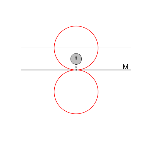
Figure 2: Figure for proof of Lemma 4. $x$ is a point in the support $M\oplus\sigma$. $y$ is the projection of $x$ onto $M$. The two spheres are tangent to $M$ at $y$ and have radius $\kappa$.

3 Minimax Lower Bound

In this section we derive a lower bound on the minimax rate of convergence for this problem. We will make use of the following result due to LeCam (1973). The following version is from Lemma 1 of Yu (1997).

Lemma 5 (Le Cam 1973)

Let ${\cal Q}$ be a set of distributions. Let $\theta(Q)$ take values in a metric space with metric $\rho$. Let $Q_{0},Q_{1}\in{\cal Q}$ be any pair of distributions in ${\cal Q}$. Let $Y_{1},\ldots,Y_{n}$ be drawn iid from some $Q\in{\cal Q}$ and denote the corresponding product measure by $Q^{n}$. Let $\widehat{\theta}(Y_{1},\ldots,Y_{n})$ be any estimator. Then

$$\sup_{Q\in{\cal Q}}\mathbb{E}_{Q^{n}}\Bigl{[}\rho(\widehat{\theta}(Y_{1},\ldots,Y_{n}),\theta(Q))\Bigr{]}\geq\rho\bigl{(}\theta(Q_{0}),\theta(Q_{1})\bigr{)}\ ||Q_{0}^{n}\wedge Q_{1}^{n}||.$$ (18)

To get a useful bound from Le Cam’s lemma, we need to construct an appropriate pair $Q_{0}$ and $Q_{1}$. This is the topic of the next subsection.

3.1 A Geometric Construction

In this section, we construct a pair of manifolds $M_{0},M_{1}\in{\cal M}(\kappa)$ and corresponding distributions $Q_{0},Q_{1}$ for use in Le Cam’s lemma. An informal description is as follows. Roughly speaking, $M_{0}$ and $M_{1}$ minimize the Hellinger distance $h(Q_{0},Q_{1})$ subject to their Hausdorff distance $H(M_{0},M_{1})$ being equal to a given value $\gamma$.

Let

$$M_{0}=\Bigl{\{}(u_{1},\ldots,u_{d},0,\ldots,0):\ -1\leq u_{j}\leq 1,\ 1\leq j\leq d\Bigr{\}}$$ (19)

be a $d$-dimensional hyperplane in $\mathbb{R}^{D}$. Hence $\Delta(M_{0})=\infty$. Place a hypersphere of radius $\kappa$ below $M_{0}$. Push the sphere upwards into $M_{0}$ causing a bump of height $\gamma$ at the origin. This creates a new manifold $M_{0}^{\prime}$ such that $H(M_{0},M_{0}^{\prime})=\gamma$. However, $M_{0}^{\prime}$ is not smooth. We will roll a sphere of radius $\kappa$ around $M_{0}^{\prime}$ to get a smooth manifold $M_{1}$ as in Figure 3. The formal details of the construction are in Section 7.2.

A

B

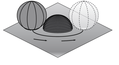
C

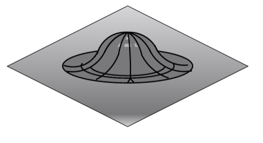
D

Figure 3: A sphere of radius $\kappa$ is pushed upwards into the plane $M_{0}$ (panel A). The resulting manifold $M_{0}^{\prime}$ is not smooth (panel B). A sphere is then rolled around the manifold (panel C) to produce a smooth manifold $M_{1}$ (panel D).

Theorem 6

Let $\gamma$ be a small positive number. Let $M_{0}$ and $M_{1}$ be as defined in Section 7.2. Let $Q_{i}$ be the corresponding distributions on $M_{i}\oplus\sigma$ for $i=0,1$. Then:

1. $\Delta(M_{i})\geq\kappa$, $i=0,1$.

2. $H(M_{0},M_{1})=\gamma$.

3. $\int|q_{0}-q_{1}|=O(\gamma^{(d+2)/2})$.

Proof  See Section 7.2.  

3.2 Proof of the Lower Bound

Now we are in a position to prove the first theorem. Let us first restate the theorem.

Theorem 1. There is a constant $C>0$ such that, for all large $n$,

$$\inf_{\widehat{M}}\sup_{Q\in{\cal Q}}\mathbb{E}_{Q}\left[H(\widehat{M},M)\right]\geq Cn^{-\frac{2}{2+d}}$$ (20)

where the infimum is over all estimators $\widehat{M}$.

Proof of Theorem 1. Let $M_{0}$ and $M_{1}$ be as defined in Section 3.1. Let $Q_{i}$ be the uniform distribution on $M_{i}\oplus\sigma$, $i=0,1$. Let $q_{i}$ be the density of $Q_{i}$ with respect to Lebesgue measure $\nu_{D}$, $i=0,1$. Then, from Theorem 6, $H(M_{0},M_{1})=\gamma$ and $\int|q_{0}-q_{1}|=O(\gamma^{(d+2)/2})$. Le Cam’s lemma then gives, for any $\widehat{M}$,

$$\sup_{Q\in{\cal Q}}\mathbb{E}_{Q^{n}}[H(M,\widehat{M})]\geq H(M_{0},M_{1})\ ||Q_{0}^{n}\wedge Q_{1}^{n}||\geq\gamma(1-c\gamma^{(d+2)/2})^{2n}$$

where we used equation (13). Setting $\gamma=n^{-2/(d+2)}$ yields the result. $\blacksquare$

4 Upper bound

To establish the upper bound, we will construct an estimator that achieves the appropriate rate. The estimator is intended only for the theoretical purpose of establishing the rate. (A simpler but non-optimal method is discussed in Section 5.) Recall that ${\cal M}={\cal M}(\kappa)$ is the set of all $d$-dimensional submanifolds $M$ contained in ${\cal K}$ such that $\Delta(M)\geq\kappa>0$. Before proceeding, we need to discuss sieve maximum likelihood.

Sieve Maximum Likelihood. Let ${\cal P}$ be any set of distributions such that each $P\in{\cal P}$ has a density $p$ with respect to Lebesgue measure $\nu_{D}$. Recall that $h$ denotes Hellinger distance. A set of pairs of functions ${\cal B}=\{(\ell_{1},u_{1}),\ldots,(\ell_{N},u_{N})\}$ is an $\epsilon$-Hellinger bracketing for ${\cal P}$ if, (i) for each $p\in{\cal P}$ there is a $(\ell,u)\in{\cal B}$ such that $\ell(y)\leq p(y)\leq u(y)$ for all $y$ and (ii) $h(\ell,u)\leq\epsilon$. The logarithm of the size of the smallest $\epsilon$-bracketing is called the bracketing entropy and is denoted by ${\cal H}_{[\,]}(\epsilon,{\cal P},h)$.

We will make use of the following result which is Example 4 of Shen and Wong (1995).

Theorem 7 (Shen and Wong (1995))

Let $\epsilon_{n}$ solve the equation ${\cal H}_{[\,]}(\epsilon_{n},{\cal P},h)=n\epsilon_{n}^{2}$. Let $(\ell_{1},u_{1}),\ldots,(\ell_{N},u_{N})$ be an $\epsilon_{n}$ bracketing where $N={\cal H}_{[\,]}(\epsilon_{n},{\cal P},h)$. Define the set of densities $S^{*}_{n}=\{p_{1}^{*},\ldots,p_{N}^{*}\}$ where $p_{t}^{*}=u_{t}/\int u_{t}$. Let $\widehat{p}^{*}$ maximize the likelihood $\prod_{i=1}^{n}p_{t}^{*}(Y_{i})$ over the set $S^{*}_{n}$. Then

$$\sup_{P\in{\cal P}}P^{n}\left(\{h(p,\widehat{p}^{*})\geq\epsilon_{n}\}\right)\leq c_{1}e^{-c_{2}n\epsilon_{n}^{2}}.$$ (21)

The sequence $\{S_{n}^{*}\}$ in Theorem 7 is called a sieve and the estimator $\widehat{p}^{*}$ is called a sieve-maximum likelihood estimator. The estimator $\widehat{p}^{*}$ need not be in ${\cal P}$. We will actually need an estimator that is contained in ${\cal P}$. We may construct one as follows. Let $\widehat{p}^{*}$ be the sieve mle corresponding to $S_{n}^{*}$. Then $\widehat{p}^{*}=p_{t}^{*}$ for some $t$. Let $(\widehat{\ell},\widehat{u})\equiv(\ell_{t},u_{t})$ be the corresponding bracket.

Lemma 8

Assume the conditions in Theorem 7. Let $\widehat{p}$ be any density in ${\cal P}$ such that $\widehat{\ell}\leq\widehat{p}\leq\widehat{u}$. If $\epsilon_{n}\leq 1$ then

$$\sup_{P\in{\cal P}}P^{n}\left(\{h(p,\widehat{p})\geq c\epsilon_{n}\}\right)\leq c_{1}e^{-c_{2}n\epsilon_{n}^{2}}.$$ (22)

Proof  By the triangle inequality, $h(p,\widehat{p})\leq h(p,\widehat{p}^{*})+h(\widehat{p},\widehat{p}^{*})=h(p,\widehat{p}^{*})+h(\widehat{p},u_{t}/\int u_{t})$ where $\widehat{p}^{*}=u_{t}/\int u_{t}$ for some $t$. From Theorem 7, $h(p,\widehat{p}^{*})\leq\epsilon_{n}$ with high probability. Thus we need to show that $h(\widehat{p},u_{t}/\int u_{t})\leq C\epsilon_{n}$. It suffices to show that, in general, $h(p,u/\int u)\leq C\,h(\ell,u)$ whenever $\ell\leq p\leq u$.

Let $(\ell,u)$ be a bracket and let $\delta^{2}=h^{2}(\ell,u)\leq 1$. Let $\ell\leq p\leq u$. We claim that $h^{2}(p,u/\int u)\leq 4\delta^{2}$. (Taking $\delta=\epsilon_{n}$ then proves the result.) Let $c^{2}=\int u$. Then $1\leq c^{2}=\int u=\int p+\int(u-p)=1+\int(u-p)=1+\ell_{1}(u,p)\leq 1+2h(u,\ell)=1+2\delta$. Now,

$$h^{2}\left(p,\frac{u}{\int u}\right) = \int(\sqrt{u}/c-\sqrt{p})^{2}=\frac{1}{c^{2}}\int(\sqrt{u}-c\sqrt{p})^{2}\leq\int(\sqrt{u}-c\sqrt{p})^{2}$$

$$= \int((\sqrt{u}-\sqrt{p})+(c-1)\sqrt{p})^{2}\leq 2\int(\sqrt{u}-\sqrt{p})^{2}+2(c-1)^{2}$$

$$\leq 2\delta^{2}+2(\sqrt{1+2\delta}-1)^{2}\leq 2\delta^{2}+2\delta^{2}=4\delta^{2}$$

where the last inequality used the fact that $\delta\leq 1$.  

In light of the above result, we define modified maximum likelihood sieve estimator $\widehat{p}$ to be any $p\in{\cal P}$ such that $\widehat{\ell}\leq\widehat{p}\leq\widehat{u}$. For simplicity, in the rest of the paper, we refer to the modified sieve estimator $\widehat{p}$, simply as the maximum likelihood estimator (mle).

Outline of proof.

We are now ready to find an estimator $\widehat{M}$ that converges at the optimal rate (up to logarithmic terms.) Our strategy for estimating $M$ has the following steps:

1. We split the data into two halves.

2. Let $\widetilde{Q}$ be the maximum likelihood estimator using the first half of the data. Define $\widetilde{M}$ to be the corresponding manifold. We call $\widetilde{M}$, the pilot estimator. We show that $\widetilde{M}$ is a consistent estimator of $M$ that converges at a sub-optimal rate $a_{n}=n^{-\frac{2}{D(d+2)}}$. To show this we:

   1. Compute the Hellinger bracketing entropy of ${\cal Q}$. (Theorem 9, Lemmas 10 and 11).

   2. Establish the rate of convergence of the mle in Hellinger distance, using the bracketing entropy and Theorem 7.

   3. Relate the Hausdorff distance to the Hellinger distance and hence establish the rate of convergence $a_{n}$ of the mle in Hausdorff distance. (Lemma 13).

   4. Conclude that the true manifold is contained, with high probability, in ${\cal M}_{n}=\{M\in{\cal M}(\kappa):\ H(M,\widetilde{M})\leq a_{n}\}$ (Lemma 14). Hence, we can now restrict attention to ${\cal M}_{n}$.

3. To improve the pilot estimator, we need to control the relationship between Hellinger and Hausdorff distance and thus need to work over small sets on which the manifold cannot vary too greatly. Hence, we cover the pilot estimator with long, thin slabs $R_{1},\ldots,R_{N}$. We do this by first covering $\widetilde{M}$ with spheres $\gimel_{1},\ldots,\gimel_{N}$ of radius $\delta_{n}=O((\log n/n)^{1/(2+d)})$. We define a slab $R_{j}$ to be the union of fibers of size $b=\sigma+a_{n}$ within one of the spheres: $R_{j}=\cup_{x\in\gimel_{j}}L_{b}(x,\widetilde{M})$. We then show that:

   1. The set of fibers on $\widetilde{M}$ cover each $M\in{\cal M}_{n}$ in a nice way. In particular, if $M\in{\cal M}_{n}$ then each fiber from $\widetilde{M}$ is nearly normal to $M$. (Lemma 15).

   2. As $M$ cuts through a slab, it stays nearly parallel to $\widetilde{M}$. Roughly speaking, $M$ behaves like a smooth, nearly linear function within each slab. (Lemma 16).

4. Using the second half of the data, we apply maximum likelihood within each slab. This defines estimators $\widehat{M}_{j}$, for $1\leq j\leq N$. We show that:

   1. The entropy of the set of distributions within a slab is very small. (Lemma 18).

   2. Because the entropy is small, the maximum likelihood estimator within a slab converges fairly quickly in Hellinger distance. The rate is $\epsilon_{n}=(\log n/n)^{1/(2+d)}$. (Lemma 19).

   3. Within a slab, there is a tight relationship between Hellinger distance and Hausdorff distance. Specifically, $H(M_{1},M_{2})\leq c\,h^{2}(Q_{1},Q_{2})$. (Lemma 20).

   4. Steps (4b) and (4c) imply that $H(M\cap R_{j},\widehat{M}_{j})=O_{P}(\epsilon_{n}^{2})=O_{P}((\log n/n)^{2/(d+2)})$.

5. Finally we define $\widehat{M}=\bigcup_{j=1}^{N}\widehat{M}_{j}$ and show that $\widehat{M}$ converges at the optimal rate because each $\widehat{M}_{j}$ does within its own slab.

The reason for getting a preliminary estimator and then covering the estimator with thin slabs is that, within a slab, there is a tight relationship between Hellinger distance and Hausdorff distance. This is not true globally but only in thin slabs. Maximum likelihood is optimal with respect to Hellinger distance. Within a slab, this allows us to get optimal rates in Hausdorff distance.

Step 1: Data Splitting

For simplicity assume the sample size is even and denote it by $2n$. We split the data into two halves which we denote by $X=(X_{1},\ldots,X_{n})$ and $Y=(Y_{1},\ldots,Y_{n})$.

Step 2: Pilot Estimator

Let $\widetilde{q}$ be the maximum likelihood estimator over ${\cal Q}$. Let $\widetilde{M}$ be the corresponding manifold. To study the properties of $\widetilde{M}$ requires two steps: computing the bracketing entropy of ${\cal Q}$ and relating $H(M,\widetilde{M})$ to $h(q,\widetilde{q})$. The former allows us to apply Theorem 7 to bound $h(q,\widetilde{q})$, and the latter allows us to control the Hausdorff distance.

Step 2a: Computing the Entropy of ${\cal Q}$. To compute the entropy of ${\cal Q}$ we start by constructing a finite net of manfolds to cover ${\cal M}(\kappa)$. A finite set of $d$-manifolds $\mathbb{M}_{\gamma}=\{M_{1},\ldots,M_{N}\}$ is a $\gamma$-net (or a $\gamma$-cover) if, for each $M\in{\cal M}$ there exists $M_{j}\in\mathbb{M}_{\gamma}$ such that $H(M,M_{j})\leq\gamma$. Let $N(\gamma)=N(\gamma,{\cal M},H)$ be the size of the smallest covering set, called the (Hausdorff) covering number of ${\cal M}$.

Theorem 9

The Hausdorff covering number of ${\cal M}$ satisfies the following:

$$N(\gamma)\equiv N(\gamma,{\cal M},H)\leq c_{1}\,\kappa_{2}(\kappa,d,D)\exp\left(\kappa_{3}(\kappa,d,D)\,\gamma^{-d/2}\right)\equiv c\exp\left(c^{\prime}\gamma^{-d/2}\right)$$ (23)

where $\kappa_{2}(\kappa,d,D)={\binom{D}{d}}^{(c_{2}/\kappa)^{D}}$ and $\kappa_{3}(\kappa,d,D)=2^{d/2}(D-d)(c_{2}/\kappa)^{D}$, for a constant $c_{2}$ that depends only on $\kappa$ and $d$.

Proof  Recall that the manifolds in ${\cal M}$ all lie within ${\cal K}$. Consider any hypercube containing ${\cal K}$. Divide this cube into a grid of $J=(2c/\kappa)^{D}$ sub-cubes $\{C_{1},\ldots,C_{J}\}$ of side length $\kappa/c$, where $c\geq 4$ is a positive constant chosen to be sufficiently large. Our strategy is to show that within each of these cubes, the manifold is the graph of a smooth function. We then only need count the number of such smooth functions.

In thinking about the manifold as (locally) the graph of a smooth function, it helps to be able to translate easily between the natural coordinates in ${\cal K}$ and the domain-range coordinates of the function. To that end, within each subcube $C_{j}$ for $j\in\left\{1,\ldots,J\right\}$, we define $K=\binom{D}{d}$ coordinate frames, $F_{jk}$ for $k\in\left\{1,\ldots,K\right\}$, in which $d$ out of $D$ coordinates are labeled as “domain” and the remaining $D-d$ coordinates are labeled as “range.”

Each frame is associated with a relabeling of the coordinates so that the $d$ “domain” coordinates are listed first and $D-d$ “range” coordinates last. That is, $F_{jk}$ is defined by a one-to-one correspondence between $x\in C_{j}$ and $(u,v)\in\pi_{jk}(x)$ where $u\in\mathbb{R}^{d}$ and $v\in\mathbb{R}^{D-d}$ and $\pi_{jk}(x_{1},\ldots,x_{D})=(x_{i_{1}},\ldots,x_{i_{d}},x_{j_{1}},\ldots,x_{j_{D-d}})$ for domain coordinate indices $i_{1}<\ldots<i_{d}$ and range coordinate indices $j_{1}<\ldots<j_{D-d}$.

We define ${\rm domain}(F_{jk})=\{u\in\mathbb{R}^{d}:\;\exists v\in\mathbb{R}^{D-d}\ \mbox{such that}\ (u,v)\in F_{jk}\}$, and let ${\cal G}_{jk}$ denote the class of functions defined on ${\rm domain}(F_{jk})$ whose second derivative (i.e., second fundamental form) is bounded above by a constant $C(\kappa)$ that depends only on $\kappa$. To say that a set $R\subset C_{j}$ is the graph of a function on a $d$-dimensional subset of the coordinates in $C_{j}$ is equivalent to saying that for some frame $F_{jk}$ and some set $A\subset{\rm domain}(F_{jk})$, $R=\pi_{jk}^{-1}\left\{(u,f(u)):\;u\in A\right\}$.

We will prove the theorem by establishing the following claims.

Claim 1. Let $M\in{\cal M}$ and $C_{j}$ be a subcube that intersects $M$. Then: (i) for at least one $k\in\{1,\ldots,K\}$, the set $M\cap C_{j}$ is the graph of a function (i.e., single-valued mapping) defined on a set ${\cal A}\subset{\rm domain}(F_{jk})$, of the form $(u_{1},\ldots,u_{d})\mapsto\pi^{-1}_{jk}((u,f(u)))$ for some function $f$ on ${\cal A}$, and (ii) this function lies in ${\cal G}_{jk}$.

Claim 2. ${\cal M}$ is in one-to-one correspondence with a subset of ${\cal G}=\prod_{j=1}^{J}\bigcup_{k=1}^{K}{\cal G}_{jk}$.

Claim 3. The $L^{\infty}$ covering number of ${\cal G}$ satisfies

$$N(\gamma,{\cal G},L^{\infty})\leq c_{1}\binom{D}{d}^{(2c/\kappa)^{D}}\exp\left((D-d)(2c/\kappa)^{D}\gamma^{-d/2}\right).$$

Claim 4. There is a one-to-one correspondence between an $\gamma/2$ $L^{\infty}$-cover of ${\cal G}$ and an $\gamma$ Hausdorff-cover of ${\cal M}$.

Taken together, the claims imply that

$$N(\gamma,{\cal M},H)\leq c_{1}\binom{D}{d}^{(2c/\kappa)^{D}}\exp((D-d)(2c/\kappa)^{D}2^{d/2}\gamma^{-d/2}).$$

Taking $c_{2}=2c$ proves the theorem.

Proof of Claim 1. We begin by showing that (i) implies (ii). By part 1 of Lemma 3, each $M\in{\cal M}$ has curvature (second fundamental form) bounded above by $1/\kappa$. This implies that the function identified in (i) has uniformly bounded second derivative and thus lies in the corresponding ${\cal G}_{jk}$.

We prove (i) by contradiction. Suppose that there is an $M\in{\cal M}$ such that for every $j$ with $M\cap C_{j}\neq\emptyset$, the set $M\cap C_{j}$ is not the graph of a single-valued mapping for any of the $K$ coordinate frames.

Fix $j\in\{1,\ldots,J\}$. Then in each ${\rm domain}(F_{jk})$, there is a point $u$ such that $C_{j}\cap\pi_{jk}^{-1}(u\times\mathbb{R}^{D-d})$ intersects $M$ in at least two points, call them $a_{k}$ and $b_{k}$. By construction $\left\|a_{k}-b_{k}\right\|\leq\sqrt{D-d}\cdot\kappa/c$, and hence by choosing $c$ large enough (making the cubes small), part 3 of Lemma 3 tells us that $d_{M}(a_{k},b_{k})\leq 2\sqrt{D-d}\kappa/c$. Then we argue as follows:

1. By parts 2 and 3 of Lemma 3 and the fact that $C_{j}$ has diameter $\sqrt{D}\kappa/c$ and

   $$\max_{p,q\in C_{j}\cap M}\cos(\mathop{\sf angle}(T_{p}M,T_{q}M))\geq 1-\frac{2\sqrt{D}}{c}.$$

   For large enough $c$, the maximum angle between tangent vectors can be made smaller than $\pi/3$.

2. By part 2 of Lemma 3, any point $z$ along a geodesic between $a_{k}$ and $b_{k}$,

   $$\cos(\mathop{\sf angle}(T_{a_{k}}M,T_{z}M))\geq 1-\frac{2\sqrt{D-d}}{c}.$$

   It follows that there is a point in $C_{j}\cap M$ and a tangent vector $v_{k}$ at that point such that $\mathop{\sf angle}(v_{k},b_{k}-a_{k})=O(1/\sqrt{c})$.

3. We have for each of $K=\binom{D}{d}$ coordinate frames and associated tangent vectors $v_{1},\ldots,v_{K}$ that are each nearly orthogonal to at least $d$ of the others. Consequently, there are $\geq d+1$ nearly orthogonal tangent vectors of $M$ within $C_{j}$. This contradicts point 1 and proves the claim.

Proof of Claim 2. We construct the correspondence as follows. For each cube $C_{j}$, let $k_{j}^{*}$ be the smallest $k$ such that $M\cap C_{j}$ is the graph of a function $\phi_{jk}\in{\cal G}_{jk}$ as in Claim 1. Map $M$ to $\varphi=(\phi_{1k_{1}^{*}},\ldots,\phi_{Jk_{J}^{*}})$, and let ${\cal F}\subset{\cal G}$ be the image of this map. If $M\neq M^{\prime}\in{\cal M}$, then the corresponding $\varphi$ and $\varphi^{\prime}$ must be distinct. If not, then $M\cap C_{j}=M^{\prime}\cap C_{j}$ for all $j$, contradicting $M\neq M^{\prime}$. The correspondence from ${\cal M}$ to ${\cal F}$ is thus a one-to-one correspondence.

Proof of Claim 3. From the results in Birman and Solomjak (1967), the set of functions defined on a pre-compact $d$-dimensional set that take values in a fixed dimension space $\mathbb{R}^{m}$ with uniformly bounded second derivative has $L^{\infty}$ covering number bounded above by $c_{1}e^{m(1/\gamma)^{d/2}}$ for some $c_{1}$. Part 1 of Lemma 3 shows that each $M\in{\cal M}$ has curvature (second fundamental form) bounded above by $1/\kappa$, so each ${\cal G}_{jk}$ satisfies Birman and Solomjak’s conditions. Hence, $N(\gamma,{\cal G}_{jk},L^{\infty})\leq c_{1}e^{(D-d)(1/\gamma)^{d/2}}$. Because all the ${\cal G}_{jk}$’s are disjoint, simple counting arguments show that $N(\gamma,{\cal G},L^{\infty})=\left(\binom{D}{d}N(\gamma,{\cal G}_{jk},L^{\infty})\right)^{J}$, where $J$ is the number of cubes defined above. The claim follows. (Note that the functions in Claim 1 are defined on a subset of ${\rm domain}(F_{jk})$. But because all such functions have an extension in ${\cal G}_{jk}$, a covering of ${\cal G}_{jk}$ also covers these functions defined on restricted domains.)

Proof of Claim 4. First, note that if two functions are less than $\gamma$ distant in $L^{\infty}$, their graphs are less than $\gamma$ distant in Hausdorff distance, and vice versa. This implies that a $\gamma$ $L^{\infty}$-cover of a set of functions corresponds directly to an $\gamma$ Hausdorff-cover of the set of the functions’ graphs. Hence, in the argument that follows, we can work with functions or graphs interchangeably.

For $k\in\{1,\ldots,K\}$, let ${\cal G}_{jk}^{\gamma}$ be a minimal $L^{\infty}$ cover of ${\cal G}_{jk}$ by $\gamma/2$ balls; specifically, we assume that ${\cal G}_{jk}^{\gamma}$ is the set of centers of these balls. For each $g_{jk}\in{\cal G}_{jk}^{\gamma}$, define $f_{jk}(u)=\pi^{-1}_{jk}(u,g_{jk}(u))$. For every $j$, choose one such $f_{jk}$, and define a set $M^{\prime}=\bigcup_{j}(C_{j}\cap{\rm range}(f_{jk_{j}}))$, which is a union of manifolds with boundary that have curvature bounded by $1/\kappa$. That is, such an $M^{\prime}$ is piecewise smooth (smooth within each cube) but may fail to satisfy $\Delta(M^{\prime})\geq\kappa$ globally. Let ${\cal A}$ be the collection of $M^{\prime}$ constructed this way. There are $N(\gamma/2,{\cal G},L^{\infty})$ elements in this collection.

By construction and Claim 2, for each $M\in{\cal M}$, there exists an $M^{\prime}\in{\cal A}$ such that $H(M,M^{\prime})\leq\gamma/2$. In other words, the set of $\gamma/2$ Hausdorff balls around the manifolds in ${\cal A}$ covers ${\cal M}$ but the elements of ${\cal A}$ are not themselves necessarily in ${\cal M}$. Let $B_{H}(A,\gamma/2)$ denote the set of all $d$-manifolds $M\in{\cal M}$ such that $H(A,M)\leq\gamma/2$. Let

$${\cal A}_{0}=\Bigl{\{}A\in{\cal A}:\ B_{H}(A,\gamma/2)\cap{\cal M}\neq\emptyset\Bigr{\}}.$$ (24)

For each $A\in{\cal A}_{0}$, choose some $\widetilde{A}\in B_{H}(A,\gamma/2)\cap{\cal M}$. By the triangle inequality, the set $\{\widetilde{A}:\ A\in{\cal A}_{0}\}$ forms an $\gamma$ Hausdorff-net for ${\cal M}$. This proves the claim.  

We are almost ready to compute the entropy. We will need the following lemma.

Lemma 10

Let $0<\gamma<\kappa-\sigma$. There exists a constant $K>0$ (depending only on ${\cal K},\kappa$ and $\sigma$) such that, for any $M_{1},M_{2}\in{\cal M}(\kappa)$, $H(M_{1},M_{2})\leq\gamma$ implies that $|V(M_{1}\oplus\sigma)-V(M_{2}\oplus\sigma)|\leq K\gamma$. Also, for any $M\in{\cal M}(\kappa)$, $|V(M\oplus(\sigma+\gamma))-V(M\oplus\sigma)|\leq K\gamma$.

Proof  Let $S_{j}=M_{j}\oplus\sigma$, $j=1,2$. Then, using (14),

$$S_{2}\subset M_{1}\oplus(\sigma+\gamma)=\bigcup_{u\in M_{1}}L_{\sigma+\gamma}(u).$$ (25)

Hence, uniformly over ${\cal M}$,

$$V(S_{2})\leq\int_{M_{1}}\nu_{D-d}(L_{\sigma+\gamma}(u))d\mu_{M_{1}}\leq\int_{M_{1}}\nu_{D-d}(L_{\sigma}(u))d\mu_{M_{1}}+K\gamma=V(S_{1})+K\gamma$$

since $\nu_{D-d}(B(u,\sigma+\gamma))\leq\nu_{D-d}(B(u,\sigma))+K\gamma$ for some $K>0$ not depending on $M_{1}$ or $M_{2}$. By a symmetric argument, $V(S_{1})\leq V(S_{2})+K\gamma$. Hence, $|V(M_{1}\oplus\sigma)-V(M_{2}\oplus\sigma)|\leq K\gamma$. The second statement is proved in a similar way.  

Now we construct a Hellinger bracketing. Let $\gamma=\epsilon^{2}$. Let $\mathbb{M}_{\gamma}=\{M_{1},\ldots,M_{N}\}$ be a $\gamma$-Hausdorff net of manifolds. Thus, by Theorem 9, $N=N(\epsilon^{2},{\cal M},H)\leq c_{1}e^{c_{2}(1/\epsilon)^{d}}$. Let $\omega$ denote the volume of a sphere of radius $\sigma$. Let $q_{j}$ be the density corresponding to $M_{j}$. Define

$$u_{j}(y)=\left(q_{j}(y)+\frac{2\epsilon^{2}}{V(M_{j}\oplus(\sigma+\epsilon^{2}))}\right)I(y\in M_{j}\oplus(\sigma+\epsilon^{2}))$$

and

$$\ell_{j}(y)=\left(q_{j}(y)-\frac{2\epsilon^{2}}{V(M_{j}\oplus(\sigma-\epsilon^{2}))}\right)I(y\in M_{j}\oplus(\sigma-\epsilon^{2})).$$

Let ${\cal B}=\{(\ell_{1},u_{1}),\ldots,(\ell_{N},u_{N})\}$.

Lemma 11

${\cal B}$ is an $\epsilon$-Hellinger bracketing of ${\cal Q}$. Hence, ${\cal H}_{[\,]}(\epsilon,{\cal Q},h)\leq C(1/\epsilon)^{d}$.

Proof  Let $M\in{\cal M}(\kappa)$ and let $Q=Q_{M}$ be the corresponding distribution. Let $q$ be the density of $Q$. $Q$ is supported on $S=M\oplus\sigma$. There exists $M_{j}\in\mathbb{M}_{\gamma}$ such that $H(M,M_{j})\leq\epsilon^{2}$. Let $y$ be in $S$. Then there is a $x\in M$ such that $||y-x||\leq\sigma$. There is a $x^{\prime}\in M_{j}$ such that $||x-x^{\prime}||\leq\epsilon^{2}$. Hence, $d(y,M_{j})\leq\sigma+\epsilon^{2}$ and thus $y$ is in the support of $u_{j}$. Now, for $y\in S$, $u_{j}(y)-q(y)=2\epsilon^{2}/V(M_{j}\oplus(\sigma+\epsilon^{2}))\geq 0$. Hence, $q(y)\leq u_{j}(y)$. By a similar argument, $\ell_{j}(y)\leq q(y)$. Thus ${\cal B}$ is a bracketing. Now

$$\ell_{1}(\ell_{j},u_{j}) = \int u_{j}-\int\ell_{j}=\left(1+\frac{2K\epsilon^{2}}{\omega}\right)-\left(1-\frac{2K\epsilon^{2}}{\omega}\right)=\frac{4K\epsilon^{2}}{\omega}.$$

Finally, by (11), $h(u_{j},\ell_{j})\leq\sqrt{\ell_{1}(\ell_{j},u_{j})}=C\epsilon$. Thus ${\cal B}$ is a $C\epsilon$-Hellinger bracketing.  

Step 2b. Hellinger Rate.

Lemma 12

Let $\widetilde{Q}$ be the mle. Then

$$\sup_{Q\in{\cal Q}}Q^{n}\left(\left\{h(Q,\widetilde{Q})>C_{0}n^{-\frac{1}{d+2}}\right\}\right)\leq\exp\left\{-Cn^{\frac{d}{2+d}}\right\}.$$

Proof  We have shown (Lemma 11) that ${\cal H}_{[\,]}(\epsilon,{\cal Q},h)\leq C(1/\epsilon)^{d}$. Solving the equation $H_{[\,]}(\epsilon_{n},{\cal Q},h)=n\,\epsilon_{n}^{2}$ from Theorem 7 we get $\epsilon_{n}=(1/n)^{1/(d+2)}$. From Lemma 8, for all $Q$

$$Q^{n}\left(\left\{h(Q,\widetilde{Q})>C_{0}n^{-\frac{1}{d+2}}\right\}\right)\leq c_{1}e^{-c_{2}n\epsilon_{n}^{2}}=\exp\left\{-Cn^{\frac{d}{2+d}}\right\}.$$

 

Step 2c. Relating Hellinger Distance and Hausdorff Distance.

Lemma 13

Let $c=(\kappa-\sigma)\sqrt{\pi}C_{*}/(2\,\Gamma(D/2+1))$. If $M_{1},M_{2}\in{\cal M}(\kappa)$ and $h(Q_{1},Q_{2})<c$ then

$$H(M_{2},M_{2})\leq\left[\frac{2}{\sqrt{\pi}}\left(\frac{\Gamma(D/2+1)}{C_{*}}\right)^{1/D}\right]h^{\frac{1}{D}}(Q_{1},Q_{2})$$

Proof  Let $b=H(M_{1},M_{2})$ and $\gamma=\min\{\kappa-\sigma,b\}$. Let $S_{1},S_{2}$ be the supports of $Q_{1}$ and $Q_{2}$. Because $H(M_{1},M_{2})=b$, we can find points $x\in M_{1}$ and $y\in M_{2}$ such that $\left\|y-x\right\|=b$. Note that $T_{x}M_{1}$ and $T_{y}M_{2}$. are parallel, otherwise we could move $x$ or $y$ and increase $\left\|y-x\right\|$. It follows that the line segment $[x,y]$ is along a common normal vector of the two manifolds and we can write $y=x\pm bu$ for some $u\in L_{\sigma}(u,M)$. Without loss of generality, assume that $y=x+bu$. Let $x^{\prime}=x+\sigma u$ and $y^{\prime}=y+\sigma u$. Hence, $x^{\prime}\in\partial S_{1}$, $y^{\prime}\in\partial S_{2}$ and $||x^{\prime}-y^{\prime}||=b$. Note that $\partial S_{1}$ and $\partial S_{2}$ are themselves smooth $D$-manifolds with $\Delta(\partial S_{i})\geq\kappa-\sigma>0$.

We now make the following three claims:

1. $y^{\prime}\in S_{2}-S_{1}$.

2. $(x^{\prime},y^{\prime}]\subset S_{2}-S_{1}$

3. $\mathop{\rm interior}B\left(\frac{x^{\prime}+y^{\prime}}{2},\frac{\gamma}{2}\right)\subset S_{2}-S_{1}$

First, note that $y^{\prime}$ differs from $y$ along a fiber of $M_{2}$ by exactly $\sigma$, therefore $[x^{\prime},y^{\prime}]\subset S_{2}$. Second, because $x^{\prime}\in\partial S_{1}$, there is a neighborhood of $x^{\prime}$ in $[x^{\prime},y^{\prime}]$ that is not contained in $S_{1}$. Hence, if there is a point in $S_{1}\cap[x^{\prime},y^{\prime}]$ there must be a point $z^{\prime}\in\partial S_{1}\cap[x^{\prime},y^{\prime}]$, with $z^{\prime}\neq x^{\prime}$. This implies the existence of two distinct points whose fibers of length less than $\kappa-\sigma$ cross, which contradicts the fact that $\Delta(\partial S_{1})\geq\kappa-\sigma$. Claims 1 and 2 follows.

Let $B=B\left(\frac{x^{\prime}+y^{\prime}}{2},\frac{\gamma}{2}\right)$. By construction, $B$ is tangent to $\partial S_{1}$ at $x^{\prime}$ and tangent to $\partial S_{2}$ at $y^{\prime}$, and $B$ contains $[x^{\prime},y^{\prime}]$. The ball has radius $\gamma/2=(1/2)\min\{\kappa-\sigma,b\}<\kappa-\sigma$. Because $B$ intersects $S_{2}-S_{1}$, the interior of $B$ cannot intersect either $\partial S_{1}$ or $\partial S_{2}$. Claim 3 follows by a similar argument as in the proof of Claim 2. (In particular, if there were a point in the interior of $B$ that is either in $S_{1}$ or outside $S_{2}$, a line segment from $(x^{\prime}+y^{\prime})/2$ to that point would have to intersect the corresponding boundary, which cannot happen.)

Now $V(B)=(\gamma/2)^{D}\pi^{D/2}/\Gamma(D/2+1)$. So

$$h(Q_{1},Q_{2}) \geq \ell_{1}(Q_{1},Q_{2})=\int|q_{1}-q_{2}|\geq\int_{S_{1}\cap S_{2}^{c}}|q_{1}-q_{2}|$$

$$= \int_{S_{1}\cap S_{2}^{c}}q_{1}=Q_{1}(S_{1}\cap S_{2}^{c})\geq C_{*}V(S_{1}\cap S_{2}^{c})=C_{*}(\gamma/2)^{D}\pi^{D/2}/\Gamma(D/2+1).$$

Hence,

$$\gamma=\min\{\kappa-\sigma,b\}\leq\left[\frac{2}{\sqrt{\pi}}\left(\frac{\Gamma(D/2+1)}{C_{*}}\right)^{1/D}\right]h^{1/D}(Q_{1},Q_{2}).$$

If $\kappa-\sigma\leq b$ this implies that $h(Q_{1},Q_{2})>c$ which contradicts the assumption that $h(Q_{1},Q_{2})<c$. Therefore, $\gamma=b$ and the conclusion follows.  

Step 2d. Computing The Hausdorff Rate of the Pilot.

Lemma 14

Let $a_{n}=\left(\frac{C_{0}}{n}\right)^{\frac{2}{D(d+2)}}$. For all large $n$,

$$\sup_{Q\in{\cal Q}}Q^{n}\left(\{H(M,\widetilde{M})>a_{n}\}\right)\leq\exp\left\{-Cn^{\frac{d}{2+d}}\right\}.$$ (26)

Proof  Follows by combining Lemma 12 and Lemma 13.  

We conclude that, with high probability, the true manifold $M$ is contained in the set ${\cal M}_{n}=\Bigl{\{}M\in{\cal M}(\kappa):\ H(\widetilde{M},M)\leq a_{n}\Bigr{\}}$.

Step 3: Cover With Slabs

Now we cover the pilot estimator $\widetilde{M}$ with (possibly overlapping) slabs. Let $\delta_{n}=\left(\frac{C\log n}{n}\right)^{\frac{1}{2+d}}$. It follows from part 6 of Lemma 3 that there exists a collection of points $F=\{x_{1},\ldots,x_{N}\}\subset\widetilde{M}$, such that $N=(c\delta_{n})^{-d}=(Cn/\log n)^{d/(2+d)}$ and such that $\widetilde{M}\subset\bigcup_{j=1}^{N}B_{D}(x_{j},c\delta)$.

Step 3a. The Fibers of $\widetilde{M}$ Cover $M$ Nicely.

Lemma 15

Let $b=\sigma+a_{n}$. For $\widetilde{x}\in\widetilde{M}$, let $L_{b}(\widetilde{x})=T_{\widetilde{x}}^{\perp}\widetilde{M}\cap B_{D}(\widetilde{x},b)$ be a fiber at $\widetilde{x}$ of size $b$. Let $M\in{\cal M}_{n}$. Then:

1. If $\widetilde{x}\in\widetilde{M}$ and $x\in M$ are such that $\left\|x-\widetilde{x}\right\|\leq a_{n}$, then ${\sf angle}(T_{x}M,T_{\widetilde{x}}\widetilde{M})<\pi/4$.

2. $L_{b}(\widetilde{x})\cap M\neq\emptyset$.

3. If $x\in L_{b}({\widetilde{x}})\cap M$, then $\left\|x-\widetilde{x}\right\|\leq 2a_{n}$.

4. For any $\widetilde{x}\in\widetilde{M}$, $\#\{L_{b}({\widetilde{x}})\cap M\}=1.$

5. We have $M\subset\bigcup_{\widetilde{x}\in\widetilde{M}}L_{b}({\widetilde{x}}).$

Proof  1. Let $x$ and $\widetilde{x}$ be as given in the statement of the lemma and let $\theta={\sf angle}(T_{x}M,T_{\widetilde{x}}\widetilde{M})$. Suppose that $\theta\geq\pi/4$. There exists unit vectors $u\in T_{\widetilde{x}}\widetilde{M}$ and $v\in T_{x}M$ such that ${\sf angle}(u,v)=\theta$. Without loss of generality, we can assume that $x=\widetilde{x}$. (The extension to the case $x\neq\widetilde{x}$ is straightforward.)

Consider the plane defined by $u$ and $v$ as in Figure 4. We assume, without loss of generality, that $(u+v)/2$ generates the $x$-axis in this plane and that $v$ lies above the $x$-axis and $u$ lies below the $x$ axis. Let $\ell$ denote the horizontal line, parallel to the $x$-axis and lying $2a_{n}$ units above the horizontal axis. Hence, $u$ and $v$ each make an angle greater than $\pi/8$ with respect to the $x$-axis.

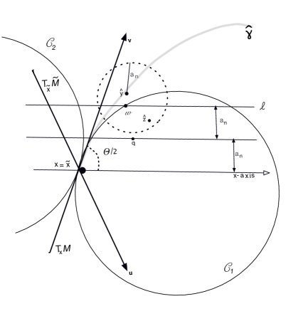
Figure 4: Figure for the proof of part 1 of Lemma 15.

Consider the two circles ${\cal C}_{1}$ and ${\cal C}_{2}$ tangent to $M$ at $x$ with radius $\kappa$ where ${\cal C}_{1}$ lies below $v$ and ${\cal C}_{2}$ lies above $v$. Let $w$ be the point at which ${\cal C}_{1}$ intersects $\ell$. The arclength of ${\cal C}_{1}$ from $x$ to $w$ is $Ca_{n}$ for some $C>1$. Let $\gamma$ be the geodesic on $M$ through $x$ with gradient $v$. The projection $\widehat{\gamma}$ of $\gamma$ into the plane must fall between ${\cal C}_{1}$ and ${\cal C}_{2}$. Let $y=\gamma(Ca_{n})$ and $\widehat{y}$ be the projection of $y$ into the plane.

Now $||y-\widetilde{x}||\geq||\widehat{y}-\widetilde{x}||\geq||w-\widetilde{x}||\geq 2a_{n}>a_{n}$. There exists $\widetilde{z}\in\widetilde{M}$ such that $||\widetilde{z}-y||\leq a_{n}$. Hence, $||\widehat{z}-\widehat{y}||\leq a_{n}$ where $\widehat{z}$ is the projection of $\widetilde{z}$ into the plane. Let $q$ be the point on the plane with coordinates $(a_{n}\sqrt{C^{2}-1},a_{n})$. Thus, $||q-\widetilde{x}||=C\,a_{n}$. Note that $\mathop{\sf angle}(\widehat{z}-\widetilde{x},u)$ is larger than the angle between $q-\widetilde{x}$ and the $x$-axis which is ${\rm arctan}\left(\frac{1}{\sqrt{C^{2}-1}}\right)\equiv\alpha>0$. Hence,

$$\mathop{\sf angle}(\widetilde{z}-\widetilde{x},u)\geq\mathop{\sf angle}(\widehat{z}-\widetilde{x},u)\geq\alpha.$$

Let $\widetilde{\gamma}$ be a geodesic on $\widetilde{M}$, parameterized by arclength connecting $\widetilde{x}$ and $\widetilde{z}$. Thus $\widetilde{\gamma}(0)=\widetilde{x}$ and $\widetilde{\gamma}(T)=\widetilde{z}$ for some $T$. There exists some $0\leq t\leq T$ such that $\gamma^{\prime}(t)\propto\widetilde{z}-\widetilde{x}$. So

$$\mathop{\sf angle}(\gamma^{\prime}(t),\gamma^{\prime}(0))=\alpha>0.$$

However, $||\widetilde{z}-\widetilde{x}||\leq(C+1)\,a_{n}$ which implies, by part 2 of Lemma 3, that $\mathop{\sf angle}(\gamma^{\prime}(t),\gamma^{\prime}(0))=O(\sqrt{a_{n}})<\alpha$ which is a contradiction.

2. For any $\widetilde{x}\in\widetilde{M}$, the closest point $x\in M$ must satisfy $\left\|x-\widetilde{x}\right\|\leq a_{n}$. Let $y$ be the projection of $x$ onto $T_{\widetilde{x}}\widetilde{M}$. Let $U=T_{\widetilde{x}}\widetilde{M}\cap B_{d}(y,a_{n})$. Let ${\rm Cyl}=\bigcup_{u\in U}B_{D}(u,3a_{n})\cap\left(T_{\widetilde{x}}\widetilde{M}\right)^{\perp}$. ${\rm Cyl}$ is a small hyper-cylinder containing $y$ and $\widetilde{x}$, with the former in the center. $M$ cannot intersect the top or bottom faces of the cylinder. Otherwise, we can find a point $p\in M$ such that $\mathop{\sf angle}(T_{\widetilde{x}}\widetilde{M},T_{p}M)>{\rm arctan}(1)=\pi/4$ contradicting 1. Thus, any path through $x$ on $M$ must intersect the sides of ${\rm Cyl}$. Hence, $L_{b}(\widetilde{x})\cap M\neq\emptyset$.

3. Let $x\in M\cap L_{b}(\widetilde{x})$. Suppose that $||x-\widetilde{x}||>2a_{n}$. There exists $q\in\widetilde{M}$ such that $||q-x||\leq a_{n}$. Note that $||q-\widetilde{x}||>a_{n}$. Now we apply part 5 Lemma 3 with $p=\widetilde{x}$ and $v=x$. This implies that $||v-p||=||x-\widetilde{x}||<a_{n}^{2}/\kappa$ which contradicts the assumption that $||x-\widetilde{x}||>2a_{n}$.

4. Suppose that more than one point of $M$ were in $L_{b}({\widetilde{x}})$. Pick two and call them $x_{1}$ and $x_{2}$. By 3, $\left\|x_{i}-\widetilde{x}\right\|\leq 2a_{n}$. It follows that $\left\|x_{1}-x_{2}\right\|\leq 4a_{n}$ and thus they are $O(a_{n})$ close in geodesic distance by part 3 of Lemma 3. Hence, there is a geodesic on $M$ connecting $x_{1}$ and $x_{2}$ that is contained strictly within the $Ca_{n}$ ball. Because $x_{2}-x_{1}$ lies in $L_{b}({\widetilde{x}})$ and is consequently orthogonal to $T_{\widetilde{x}}\widetilde{M}$, there must exist a point on the geodesic whose angle with $T_{\widetilde{x}}\widetilde{M}$ equals $\pi/2$, contradicting part 1.

5. Because $H(\widetilde{M},M)\leq a_{n}$, we have that $M\subset{\sf tube}(\widetilde{M},a_{n})$. Because $a_{n}<\kappa$, the fibers $L_{b}({\widetilde{x}})$ partition ${\sf tube}(\widetilde{M},a_{n})$. Hence, each $x\in M$ must lie on one (and only one) $L_{b}({\widetilde{x}})$.  

Step 3b. Construct slabs that cover $M$ nicely. Let $\gimel_{j}=B_{D}(x_{j},\delta_{n})\cap\widetilde{M}$. Define the slab

$$R_{j}=\bigcup_{x\in\gimel_{j}}L_{b}(x,\widetilde{M}).$$ (27)

Lemma 16

The collection of slabs $R_{1},\ldots,R_{N}$ has the following properties. Let $M\in{\cal M}_{n}$.

1. $M\subset\bigcup_{j=1}^{N}R_{j}$.

2. $M\cap R_{j}$ is function-like over $R_{j}$. That is, there exists a function $g_{j}:\gimel_{j}\to\mathbb{R}^{D-d}$ such that $M\cap R_{j}=\{g_{j}(x):\ x\in\gimel_{j}\}$.

3. For each $x\in\gimel_{j}$, $L_{b}(x)\cap M\neq\emptyset$.

4. There exists a linear function $\ell_{j}:\gimel_{j}\to\mathbb{R}^{D-d}$ such that $\sup_{x\in\gimel_{j}}||g_{j}(x)-\ell_{j}(x)||\leq C\delta_{n}^{2}$.

5. $\sup_{M\in{\cal M}_{n}}{\sf diam}(M\cap R_{j})\leq C\delta_{n}$.

Thus the slabs cover $M$ and $M$ cuts across $R_{j}$ is a function-like way. Moreover, $M\cap R_{j}$ is nearly linear.

Proof  The first three claims follow immediately from Lemma 15. In particular, $g_{j}$ in claim 2 is defined by $g_{j}(x)=\{M\cap L_{b}(x)\}$. Now we show 4. We can write $g_{j}(x)=g_{j}(x_{j})+(x-x_{j})^{T}\nabla g+\frac{1}{2}(x-x_{j})^{T}{\sf Hess}\,(x-x_{j})$ where ${\sf Hess}$ is the Hessian matrix of $g_{j}$ evaluated at some point between $x$ and $x_{j}$. By part 1 of Lemma 3, the largest eigenvalue of Hess is bounded above by $1/\kappa$. Since $||x-x_{j}||\leq c\delta_{n}^{2}$, the claim follows. Part 5 follows easily.  

Step 4: Local Conditional Likelihood

Recall that ${\cal M}_{n}=\{M\in{\cal M}(\kappa):\ H(\widetilde{M},M)\leq a_{n}\}$. Let

$${\cal Q}_{n}=\{Q_{M}:\ M\in{\cal M}_{n}\}.$$ (28)

Consider a slab $R_{j}$. For each $Q\in{\cal Q}_{n}$ define $Q_{j}\equiv Q(\cdot|R_{j})$ by $Q_{j}(A)=Q(A\cap R_{j})/Q(R_{j})$. Note that $Q_{j}$ is supported over $\mathop{\sf tube}(M,\sigma)\cap R_{j}$. Let ${\cal Q}_{n,j}=\{Q_{j}:\ Q\in{\cal Q}_{n}\}$. Before we proceed we need to establish the following.

Lemma 17

Let ${\cal I}_{j}(M)={\sf tube}(M,\sigma)\cap R_{j}$. Then there exists $c_{0}>0$ such that

$$\inf_{M\in{\cal M}_{n}}V({\cal I}_{j}(M))\geq c_{0}\delta_{n}^{d}.$$

Proof  By Lemma 16, $M\cap R_{j}$ lies in a slab of size $a_{n}$ orthogonal to $\gimel_{j}$. Because the angle between the two manifolds on this set must be no more than $\pi/4$ and because $a_{n}>\delta_{n}$, the manifold $M$ cannot intersect both the “top” and “bottom” surfaces of the slab. Hence, for large enough $C>0$, ${\cal J}_{j}=\bigcup_{x\in\gimel_{j}}B_{D}(x,\sigma/C)\subset{\cal I}_{j}$. By construction, $V({\cal I}_{j})\geq V({\cal J}_{j})\geq c\delta_{n}^{d}$.  

Step 4a. The Entropy of ${\cal Q}_{n,j}$.

Lemma 18

${\cal H}_{[\,]}(\epsilon,{\cal Q}_{n,j},h)\leq c_{1}\log(c_{2}/\epsilon)$.

Proof  We begin by creating a $\gamma$ Hausdorff net for ${\cal Q}_{n,j}$. To do this, we will parameterize the support of these distributions. Each $Q\in{\cal Q}_{n,j}$ has support in the collection ${\cal S}_{n,j}=\{(M\oplus\sigma)\cap R_{j}:\ M\in{\cal M}_{n}\}$. We will construct a $\gamma$-Hausdorff net for ${\cal S}_{n,j}$.

Let $\widetilde{x}\in\widetilde{M}$ be the center of $\gimel_{j}$. Let $y_{1},\ldots,y_{r}$ be a $c_{1}\gamma$-net of $L_{b}(\widetilde{x})$, and let $\theta_{1}<\theta_{2}<\cdots<\theta_{s}<\pi/2-\eta$ for a small, fixed $\eta>0$ where $\theta_{j}-\theta_{j-1}\leq c_{2}\gamma$. Note that $r=O(\gamma^{-(D-d)})$ and $s=O(1/\gamma)$. For every pair $y_{i}$ and $\theta_{j}$, let $M_{ij}$ be a $M\in{\cal M}_{n}$ that crosses through $y_{i}$ with ${\sf angle}(T_{y_{i}}M,T_{\widetilde{x}}\widetilde{M})=\theta_{j}$. These manifolds comprise a collection of size $O((1/\gamma)^{D-d-1})$ which we will denote by ${\sf Net}(\gamma)$.

Let $M\in{\cal M}_{n}$. Let $y$ be the point where $M$ crosses $L_{b}(\widetilde{x})$. Let $y_{i}$ be the closest point in the net to $y$ and let $\theta_{j}$ be the closest angle in the net to $\mathop{\sf angle}(T_{y}M,T_{\widetilde{x}}\widetilde{M})$. Because the angle between $M$ and $M_{ij}$ is strictly less than $\pi/4$ (part 1 of Lemma 15) and the slab $R_{j}$ has radius $\delta_{n}$, it follows that $H(M,M_{ij})\leq C_{1}\gamma+\delta_{n}C_{2}\gamma\leq C\gamma$. Hence, ${\sf Net}(\gamma)$ is a $\gamma$-Hausdorff net.

Now consider ${\sf Net}(\gamma)$ with $\gamma=\epsilon^{2}$. For each $M_{ij}\in{\sf Net}(\gamma)$ let $q_{ij}$ be the correspondng density and define $u_{ij}$ and $\ell_{ij}$ by

$$u_{ij}(y)=\left(q_{ij}(y)+\frac{C\epsilon^{2}}{V(M_{ij}\oplus(\sigma+\epsilon^{2}))}\right)I(y\in M_{ij}\oplus(\sigma+\epsilon^{2}))$$

and

$$\ell_{ij}(y)=\left(q_{ij}(y)-\frac{C\epsilon^{2}}{V(M_{ij}\oplus(\sigma-\epsilon^{2}))}\right)I(y\in M_{j}\oplus(\sigma-\epsilon^{2})).$$

Let ${\cal B}=\{(\ell_{ij},u_{ij})\}$.

Let $M\in{\cal M}_{n}$ and let $M_{ij}$ be the element of the net closest to $M$. It follows easily that $u_{ij}\geq q_{M}\geq\ell_{ij}$. Thus ${\cal B}$ is a bracketing. Now,

$$\int u_{ij}-\ell_{ij}=1+C\epsilon^{2}-(1-C\epsilon^{2})=2C\epsilon^{2}.$$

Hence, $h(u_{ij},\ell_{ij})\leq\sqrt{\int|u_{ij}-\ell_{ij}|}=\sqrt{2C}\epsilon$. Hence, ${\cal B}$ is an $\sqrt{2C}-\epsilon$-bracketing. So,

$${\cal H}_{[\,]}(\epsilon,{\cal Q}_{n,j},h)\leq(D-d-1)\log(c/\epsilon),$$ (29)

which proves the lemma.  

Step 4b. Hellinger Rate of the Conditional MLE. Let $\widehat{q}$ be the mle over ${\cal Q}_{n,j}$ using the $Y_{i}$’s in $R_{j}$. Let $\widehat{M}$ be the manifold corresponding to $\widehat{q}$ and let $\widehat{M}_{j}=\widehat{M}\cap R_{j}$.

Lemma 19

For all $Q$, all $A>0$ and all large $n$,

$$Q^{n}\left(\left\{h(Q,\widehat{Q})>\left(\frac{C_{0}\log n}{n}\right)^{\frac{1}{2+d}}\right\}\right)\leq n^{-A}.$$

Proof  Let $N_{j}$ be the number of observations from the second half of the data that are in $R_{j}$. Let $\mu_{j}=\mathbb{E}(N_{j})$ and define $m_{n}=n^{\frac{2}{2+d}}$. First, we claim that $N_{j}\geq\mu_{j}/2=O(m_{n})$ for all $j$, except on a set of probability $e^{-cn^{2/(2+d)}}$. Let $\pi_{j}=Q(R_{j})$. By Lemma 17 and Lemma 4, $\pi_{j}\geq c\delta_{n}^{d}$ for some $c>0$. Hence, $\mu_{j}\geq m_{n}$. Note that $\sigma^{2}\equiv{\sf Var}(N_{j})/n=\pi_{j}(1-\pi_{j})\leq\pi_{j}$. Let $t=\mu_{j}/2$. By Bernstein’s inequality,

$$\mathbb{P}(N_{j}\leq\mu_{j}/2)=\mathbb{P}(N_{j}-\mu_{j}\leq-\mu_{j}/2)\leq\exp\left\{-\frac{t^{2}}{2n\sigma^{2}+2t/3}\right\}\leq\exp\left\{-cn^{2/(2+d)}\right\}.$$

Hence, by the union bound,

$$\mathbb{P}(N_{j}\leq\mu_{j}/2\ {\rm for\ some\ }j)\leq\frac{1}{N}\exp\left\{-cn^{2/(2+d)}\right\}\leq\exp\left\{-c^{\prime}n^{2/(2+d)}\right\}$$

since there are $N=O(1/\delta_{n})$ slabs. Thus we can assume that there are at least order $m_{n}$ observations in each $R_{j}$.

Since ${\cal H}_{[\,]}(\epsilon,{\cal Q}_{n,j},h)\leq\log(C(1/\epsilon))$, solving the equation ${\cal H}_{[\,]}(\epsilon,{\cal Q}_{n,j},h)=m_{n}\epsilon^{2}$ we get $\epsilon_{m}\geq\sqrt{C\log m_{n}/m_{n}}=(\log n/n)^{2/(2(2+d))}=\delta_{n}$. From Lemma 8, we have, for all $Q\in Q_{n,j}$,

$$Q^{n}\left(\left\{h(Q,\widehat{Q})>\delta_{n}\right\}\right)=Q^{n}\left(\left\{h(Q,\widehat{Q})>\epsilon_{m}\right\}\right)\leq c_{1}e^{-c_{2}m_{n}\epsilon_{m}^{2}}\leq n^{-A}.$$

 

Step 4c. Relating Hausdorff Distance to Hellinger Distance Within a Slab.

Lemma 20

For each $M_{1},M_{2}\in{\cal M}_{n}$, $H(M_{1}\cap R_{j},M_{2}\cap R_{j})\leq C\,h^{2}(Q_{j1},Q_{j2})$.

Proof  Let $g_{1}$ and $g_{2}$ be defined as in Lemma 16. There exists $x\in\gimel_{j}$ such that $g_{1}(x)\in M_{1}$, $g_{2}(x)\in M_{2}$ and $||g_{1}(x)-g_{2}(x)||=\gamma$. We claim there exists $\gimel^{\prime}\subset\gimel_{j}$ such that $\inf_{x\in\gimel^{\prime}}||g_{1}(x)-g_{2}(x)||\geq\gamma/2$ and such that $V(\gimel^{\prime})\geq c\delta_{n}^{d}$. This follows since $g_{1}$ and $g_{2}$ are smooth, they both lie in a slab of size $a_{n}$ around $\gimel_{j}$ and the angle between the tangent of $g_{j}(x)$ and $\gimel_{j}$ is bounded by $\pi/4$.

Create a modified manifold $M_{2}^{\prime}$ such that $M_{2}^{\prime}$ differs from $M_{1}$ over $\gimel^{\prime}$ by a $\gamma/2$ shift orthogonal to $\gimel_{j}$ and such that $M_{2}^{\prime}$ is otherwise equal to $M_{1}$. It follows that $\ell_{1}(M_{1},M_{2})\geq\ell_{1}(M_{1},M_{2}^{\prime})$ and $h(Q_{1},Q_{2})\geq h(Q_{1},Q_{2}^{\prime})$.

Every point in the support of the conditioned distributions can be written as an ordered pair $(x,y)$ where $x\in\gimel_{j}$ and $y$ lies in a $d^{\prime}$ ball of radius $\sigma$. $M_{2}^{\prime}$ is shifted a distance of $\gamma/2$ in the direction orthogonal to $\gimel_{j}$. As a result, the $\ell_{1}$ distance between $M_{1}$ and $M_{2}^{\prime}$ equals the integral over $C^{\prime}$ of the volume difference between two $d^{\prime}$ balls of the same radius that are shifted by $\gamma/2$ relative to each other. This volume $\delta_{n}^{d}\gamma$. Hence, $V(M_{1}\cap\gimel_{j})\circ(M_{2}\cap\gimel_{j})\geq\gamma\delta_{n}^{d}$. Let $A=\{x\in\gimel_{j}:\ q_{1}>0,q_{2}=0\}$, $B=\{x\in\gimel_{j}:\ q_{1}>0,q_{2}>0\}$, $C=\{x\in\gimel_{j}:\ q_{1}=0,q_{2}>0\}$. At least one of $A$ or $B$ has volume at least $\gamma\delta_{n}^{d}/2$. Without loss of generality, assume that it is $A$. Then

$$h^{2}(q_{1},q_{2}) = \int(\sqrt{q_{1}}-\sqrt{q_{2}})^{2}\geq\int_{A}(\sqrt{q_{1}}-\sqrt{q_{2}})^{2}=\int_{A}q_{1}$$

$$\geq \frac{C_{*}c\delta_{n}^{d}\gamma}{\delta_{n}^{d}}=cC_{*}\gamma=cC_{*}H(M_{1},M_{2}).$$

 

Step 4d. The Hausdorff Rate.

Lemma 21

For any $A>0$ there exists $C_{0}$ such that

$$Q^{n}\left(\left\{H(M\cap R_{j},\widehat{M}_{j})>\left(\frac{C_{0}\log n}{n}\right)^{\frac{2}{2+d}}\right\}\right)\leq\frac{1}{n^{A}}.$$

Proof  This follows by combining Lemma 20 and Lemma 19.  

Step 5: Final Estimator

Now we can combine the estimators from the difference slabs. Let $\widehat{M}=\bigcup_{j=1}^{N}\widehat{M}_{j}$. Recall that the number of slabs is $N=(c\delta_{n})^{-d}=(Cn/\log n)^{d/(2+d)}$.

Proof of Theorem 2. Choose an $A>2/(2+d)$. We have:

$$Q^{n}\left(\left\{H(\widehat{M},M)>\left(\frac{C_{0}\log n}{n}\right)^{\frac{2}{2+d}}\right\}\right) \leq \sum_{j}Q^{n}\left(\left\{H(\widehat{M}_{j},M\cap R_{j})>\left(\frac{C_{0}\log n}{n}\right)^{\frac{2}{2+d}}\right\}\right)$$

$$\leq \frac{N}{n^{A}}$$

$$= \left(\frac{n}{C\log n}\right)^{\frac{1}{2+d}}\times\frac{1}{n^{A}}\leq\frac{c}{n^{A}}.$$

Let $r_{n}=\left(\frac{C_{0}\log n}{n}\right)^{2/(2+d)}.$ Since $M$ and $\widehat{M}$ are contained in a compact set, $H(\widehat{M},M)$ is uniformly bounded above by a constant $K_{0}$. Hence,

$$\mathbb{E}_{Q}H(\widehat{M},M) = \mathbb{E}_{Q}[H(\widehat{M},M)I(H(\widehat{M},M)>r_{n})]+\mathbb{E}_{Q}[H(\widehat{M},M)I(H(\widehat{M},M)\leq r_{n})]$$

$$\leq K_{0}\,Q^{n}(H(\widehat{M},M)>r_{n})+r_{n}$$

$$\leq \frac{c}{n^{A}}+r_{n}=O\left(\left(\frac{\log n}{n}\right)^{2/(2+d)}\right).$$

$\blacksquare$

5 A Simple, Consistent Estimator

Here we give a practical, consistent estimator, one that does not converge at the optimal rate. It is a generalization of the estimator in Genovese et al. (2010) and is similar to the estimator in Niyogi et al. (2006). Let

$$\widehat{S}=\bigcup_{i=1}^{n}B_{D}(Y_{i},\epsilon)$$ (30)

and define $\widehat{\partial S}=\partial(\widehat{S})$, $\widehat{\sigma}=\max_{y\in\widehat{S}}d(y,\widehat{\partial S})$ and

$$\widehat{M}=\Bigl{\{}y\in\widehat{S}:\ d(y,\widehat{\partial S})\geq\widehat{\sigma}-2\epsilon\Bigr{\}}.$$ (31)

Lemma 22

Let $\epsilon_{n}=C(\log n/n)^{1/D}$ in the estimator $\widehat{M}$. Then

$$H(M,\widehat{M})=O\left(\frac{\log n}{n}\right)^{1/D}$$ (32)

almost surely for all large $n$.

Before proving the lemma we need a few definitions. Following Cuevas and Rodríguez-Casal (2004), we say that a set $S$ is $(\chi,\lambda)$-standard if there exist positive numbers $\chi$ and $\lambda$ such that

$$\nu_{D}(B_{D}(y,\epsilon)\cap S)\geq\chi\ \nu_{D}(B(y,\epsilon))\ \ \ \ \ {\rm for\ all\ }y\in S,\ 0<\epsilon\leq\lambda.$$ (33)

We say that $S$ is partly expandable if there exist $r>0$ and $R\geq 1$ such that $H(\partial S,\partial(S\oplus\epsilon))\leq R\epsilon$ for all $0\leq\epsilon<r$. A standard set has no sharp peaks while a partly expandable set has not deep inlets.

Lemma 23

If $\sigma<\Delta(M)$ then $S=M\oplus\sigma$ is standard with $\chi=2^{-D}$ and $\lambda=\sigma$ and partly expandable with $r=\Delta(M)-\sigma$ and $R=1$.

Proof  Let $\chi=2^{-D}$. Let $y$ be a point in $S$ and let $\Lambda(y)\leq\sigma$ be its distance from the boundary $\partial S$. If $\Lambda(y)\geq\epsilon$ then $B_{D}(y,\epsilon)\cap S=B_{D}(y,\epsilon)$ so that $\nu_{D}(B_{D}(y,\epsilon)\cap S)=\nu_{D}(B_{D}(y,\epsilon))\geq\chi\,\nu_{D}(B_{D}(y,\epsilon))$.

Suppose that $\Lambda(y)<\epsilon$. Let $v$ be a point on the manifold closest to $y$ and let $y^{*}$ be the point on the segment joining $y$ to $v$ such that $||y-y^{*}||=\epsilon/2$. The ball $A=B_{D}(y^{*},\epsilon/2)$ is contained in both $B_{D}(y,\epsilon)$ and $S$. Hence, $\nu_{D}(B_{D}(y,\epsilon)\cap S)\geq\nu_{D}(A)\geq\chi\nu_{D}(B_{D}(y,\epsilon))$. This is true for all $\epsilon\leq\sigma$, hence $S$ is $(\chi,\lambda)$-standard for $\chi=1/2^{D}$ and $\lambda=\sigma$.

Now we show that $S$ is partly expandable. By Proposition 1 in Cuevas and Rodríguez-Casal (2004) it suffices to show that a ball of radius $r$ rolls freely outside $S$ for some $r$, meaning that, for each $y\in\partial S$, there is an $a$ such that $y\in B(a,r)\subset\overline{S^{c}}$, where $S^{c}$ is the complement of $S$. Let $O_{y}$ be the ball of radius $\Delta-\sigma$ tangent to $y$ such that $O_{y}\subset S^{c}$. Such a ball exists by virtue of the fact that $\sigma<\Delta(M)$.  

Theorem 24 (Cuevas and Rodríguez-Casal (2004))

Let $Y_{1},\ldots,Y_{n}$ be a random sample from a distribution with support $S$. Let $S$ be compact, $(\lambda,\chi)$-standard and partly expandable. Let

$$\widehat{S}=\bigcup_{i=1}^{n}B(Y_{i},\epsilon_{n})$$ (34)

and let $\widehat{\partial S}$ be the boundary of $\widehat{S}$. Let $\epsilon_{n}=C(\log n/n)^{1/D}$ with $C>(2/(\chi\ \omega_{D}))^{1/D}$ where $\omega_{D}=V(B_{D}(0,1))$. Then, with probability one,

$$H(S,\widehat{S})\leq C\left(\frac{\log n}{n}\right)^{1/D}\ \ \ {\rm and}\ \ \ \ H(\partial S,\widehat{\partial S})\leq C\left(\frac{\log n}{n}\right)^{1/D}$$ (35)

for all large $n$. Also, $S\subset\widehat{S}$ almost surely for all large $n$.

Proof of Lemma 22. Theorem 24 and Lemma 23 imply that $H(S,\widehat{S})\leq C(\log n/n)^{1/D}$ and $H(\partial S,\widehat{\partial S})\leq C(\log n/n)^{1/D}$. It follows that $\widehat{\sigma}\geq\sigma-\epsilon$. First we show that $y\in\widehat{M}$ implies that $d(y,M)\leq 4\epsilon$. Let $y\in\widehat{M}$. Then $d(y,\partial S)\geq d(y,\widehat{\partial S})-\epsilon\geq\widehat{\sigma}-2\epsilon-\epsilon\geq\sigma-\epsilon-2\epsilon-\epsilon=\sigma-4\epsilon$. So $d(y,M)=\sigma-d(y,\partial S)\leq\sigma-\sigma+4\epsilon=4\epsilon$. Now we show that $M\subset\widehat{M}$. Suppose that $y\in M$. Then,

$$d(y,\widehat{\partial S})\geq d(y,\partial S)-\epsilon=\sigma-\epsilon\geq\widehat{\sigma}-2\epsilon$$

so that $y\in\widehat{M}$. $\blacksquare$

6 Conclusion and Open Questions

We have established that the optimal rate for estimating a smooth manifold in Hausdorff distance is $n^{-\frac{2}{2+d}}$. We conclude with some comments and open questions.

1. We have assumed that the noise is perpendicular to the manifold. In current work we are deriving the minimax rate under the more general assumption that $\epsilon$ is drawn from a general, spherically symmetric distribution. We also allow the distribution along the manifold to be any smooth density bounded away from 0. The rates are quite different and the methods for proving the rates are substantially more involved. Moreover, the rates depends on the behavior of the noise density near the boundary of its support. We will report on this elsewhere.

2. Perhaps the most important open question is to find a computationally tractable estimator that achieves the optimal rate. It is possible that combining the estimator in Section 5 with one of the estimators in the computational geometry literature (Dey (2006)) could work. However, it appears that some modification of such an estimator is needed. This is a difficult question which we hope to address in the future.

3. It is interesting to note that Niyogi et al. (2006) have a Gaussian noise distribution. While it is possible to infer the homology of $M$ with Gaussian noise it is not possible to infer $M$ itself with any accuracy. The reason is that manifold estimation is similar to (and in fact, more difficult than) nonparametric regression with measurement error. In that case, it is well known that the fastest possible rates under Gaussian noise are logarithmic. This highlights an important distinction between estimating the topological structure of $M$ versus estimating $M$ in Hausdorff distance.

4. The current results take $\Delta(M)$, $d$ and $\sigma$ as known (or at least bounded by known constants). In practice these must be estimated. We do not know whether there exist minimax estimators that are adaptive over $d,\Delta(M)$ and $\sigma$.

7 Appendix

7.1 Proof of Equation 13

We will use the following two results (see Section 2.4 of Tsybakov (2008)):

$$h^{2}(P^{n},Q^{n})=2\left(1-\left[1-\frac{h^{2}(P,Q)}{2}\right]^{n}\right)$$ (36)

and

$$P\wedge Q\geq\frac{1}{2}\left(1-\frac{h^{2}(P,Q)}{2}\right)^{2}.$$ (37)

We have

$$P^{n}\wedge Q^{n} \geq \frac{1}{2}\left(1-\frac{h^{2}(P^{n},Q^{n})}{2}\right)^{2}=\frac{1}{8}\left(1-\frac{h^{2}(P,Q)}{2}\right)^{2n}$$

$$\geq \frac{1}{8}\left(1-\frac{\ell_{1}(P,Q)}{2}\right)^{2n}$$

since $h^{2}(P,Q)\leq\ell_{1}(P,Q)$.

7.2 Proof of Theorem 6

We define two manifolds $M_{1}$ and $M_{2}$ with corresponding distributions $Q_{1}$ and $Q_{2}$ such that (i) $\Delta(M_{i})\geq\kappa$ $i=1,2$, (ii) $H(M_{1},M_{2})=\gamma$ and (iii) such that the volume of $S_{1}\circ S_{2}$ is of order $\gamma^{\frac{d}{2}+1}$, where $S_{i}$ is the support of $Q_{i}$.

We write a generic $D$-dimensional vector as $y=(u,v,z)$, with $u\in\mathbb{R}^{d}$, $v\in\mathbb{R}$, $z\in\mathbb{R}^{D-d-1}$. For each $u\in\mathbb{R}^{d}$ with $||u||\leq 1$, define the disk in $\mathbb{R}^{d+1}$

$$D_{0}=\Bigl{\{}(u,0)\in\mathbb{R}^{d+1}:\ u\in B_{d}(0,1)\Bigr{\}}$$

and let

$$F_{0}=\partial\left(\bigcup_{(u,v)\in D_{0}}B_{d+1}((u,v),\kappa)\right).$$

Now define the following $d$-dimensional manifold in $\mathbb{R}^{D}$

$$M_{0} = \Bigl{\{}(u,v,0_{D-d-1}):\ (u,v)\in F_{0}\Bigr{\}}$$

$$= \Bigl{\{}(u,a(u),0_{D-d-1}):\ u\in B_{d}(0,1+\kappa)\Bigr{\}}\cup\Bigl{\{}(u,-a(u),0_{D-d-1}):\ u\in B_{d}(0,1+\kappa)\Bigr{\}}$$

where

$$a(u)=\left\{\begin{array}[]{ll}\kappa&{\rm if}\;||u||\leq 1\\ \sqrt{\kappa^{2}-(||u||-1)^{2}}&{\rm if}\;1<\ ||u||\leq 1+\kappa.\end{array}\right.$$

The manifold $M_{0}$ has no boundary and, by construction, $\Delta(M_{0})\geq\kappa$.

Now define a second manifold that coincides with $M_{0}$ but has a small perturbation:

$$M_{1} = \Bigl{\{}(u,b(u),0_{D-d-1}):\ u\in B_{d}(0,1+\kappa)\Bigr{\}}\cup\Bigl{\{}(u,-a(u),0_{D-d-1}):\ u\in B_{d}(0,1+\kappa)\Bigr{\}}$$

where

$$b(u)=\left\{\begin{array}[]{ll}\gamma+\sqrt{\kappa^{2}-||u||^{2}}&{\rm if}\;||u||\leq\frac{1}{2}\sqrt{4\gamma\kappa-\gamma^{2}}\\ 2\kappa-\sqrt{\kappa^{2}-(||u||-\sqrt{4\gamma\kappa-\gamma^{2}})^{2}}&{\rm if}\;\frac{1}{2}\sqrt{4\gamma\kappa-\gamma^{2}}<\ ||u||\leq\sqrt{4\gamma\kappa-\gamma^{2}}\\ a(u)&{\rm if}\;\sqrt{4\gamma\kappa-\gamma^{2}}<\ ||u||\leq\sqrt{4\gamma\kappa-\gamma^{2}}+\kappa.\\ \end{array}\right.$$

Note that $\Delta(M_{1})\geq\kappa$ since the perturbation is obtained using portions of spheres of radius $\kappa$. In fact

• for $||u||\leq\frac{1}{2}\sqrt{4\gamma\kappa-\gamma^{2}}$, $b(u)$ is the $d+1$-th coordinate of the “upper” portion of the $(d+1)$-dimensional sphere with radius $\kappa$ centered at $(0,\cdots,0,\gamma)$, hence $b(u)$ satisfies

  $$||u||^{2}+(b(u)-\gamma)^{2}=\kappa^{2}\qquad\mbox{with }b(u)\geq\gamma;$$

• for $\frac{1}{2}\sqrt{4\gamma\kappa-\gamma^{2}}<\ ||u||\leq\sqrt{4\gamma\kappa-\gamma^{2}}$, $b(u)$ is the $(d+1)$-th coordinate of the “lower” portion of the $(d+1)$-dimensional sphere with radius $\kappa$ centered at $(u\cdot\sqrt{4\gamma\kappa-\gamma^{2}}/||u||,2\kappa)$ (note that the center of the sphere differs according to the direction of $u$), hence $b(u)$ satisfies

  $$\left|\left|u-\frac{u}{||u||}\sqrt{4\gamma\kappa-\gamma^{2}}\right|\right|^{2}+(b(u)-2\kappa)^{2}=\kappa^{2}\qquad\mbox{with }b(u)\leq 2\kappa.$$

To summarize, $M_{0}$ and $M_{1}$ are both manifolds with no boundary, $\Delta(M_{0})\geq\kappa$ and $\Delta(M_{1})\geq\kappa$. See Figure 5. Now

$$E_{0} = M_{0}-M_{1}=\Bigl{\{}(u,a(u),0_{D-d-1}):\ u\in B_{d}(0,\sqrt{4\gamma\kappa-\gamma^{2}})\Bigr{\}}$$

$$E_{1} = M_{1}-M_{0}=\Bigl{\{}(u,b(u),0_{D-d-1}):\ u\in B_{d}(0,\sqrt{4\gamma\kappa-\gamma^{2}})\Bigr{\}}.$$

Figure 5: One section of manifolds $M_{0}$ and $M_{1}$. The common part is dashed, $E_{0}$ is dotted and $E_{1}$ solid. $R_{1}$ and $R_{2}$ denote the regions where the different definitions of the perturbation apply: $R_{1}$ is $||u||\leq\frac{1}{2}\sqrt{4\gamma\kappa-\gamma^{2}}$ while $R_{2}$ denotes $\frac{1}{2}\sqrt{4\gamma\kappa-\gamma^{2}}<||u||\leq\sqrt{4\gamma\kappa-\gamma^{2}}$.

Note that for each point $y\in E_{0}$ there exists $y^{\prime}\in E_{1}$ such that $||y-y^{\prime}||\leq|a(u)-b(u)|\leq\gamma$. Also, $y_{0}=(0,a(0),0)\in M_{0}$ has as its closest $M_{1}$ point $y_{1}=(0,b(0),0)$, so that $||y_{0}-x_{0}||=\gamma$. Hence $H(M_{0},M_{1})=H(E_{0},E_{1})=\gamma$.

To find an upper bound for $V(S_{0}\circ S_{1})$, we show that each $y=(u,v,z)\in S_{1}-S_{0}$ satisfies the following conditions:

• $u\in B_{d}(0,\sqrt{4\gamma\kappa-\gamma^{2}})$;

• $z\in B_{D-d-1}(0,\sigma)$;

• $\kappa+\sigma-||z||<v\leq\kappa+\gamma+\sigma-||z||]$.

If $y=(u,v,z)$ belongs to $S_{1}$ and has $||u||>\sqrt{4\gamma\kappa-\gamma^{2}}$, then there is a point of $M_{0}\cap M_{1}$ within distance $\sigma$, hence $y\not\in S_{1}-S_{0}$. This proves (i). Before proving (ii) and (iii), note that if $u\in B_{d}(0,\sqrt{4\gamma\kappa-\gamma^{2}})$ then

$$\kappa=a(u)\leq b(u)\leq\kappa+\gamma.$$

Now, let $y^{\prime}=(u^{\prime},b(u^{\prime}),0)\in E_{1}$ be the point in $S_{1}$ closest to $y$. We have

$$d(y,S_{1})=||y-y^{\prime}||=||u-u^{\prime}||+|v-b(u^{\prime})|+||z||\leq\sigma.$$

This gives condition (ii) above $||z||\leq\sigma$ and also

$$|v-b(u^{\prime})|\leq\sigma-||z||.$$ (38)

Since $b(u^{\prime})\leq\kappa+\gamma$, we obtain

$$v\leq b(u^{\prime})+\sigma-||z||\leq\kappa+\gamma+\sigma-||z||$$

which is the right inequality in (iii). Finally,

$$\sigma<d(y,M_{0})\leq||y-(u,a(u),0)||=|v-a(u)|+||z||$$

which implies either $v<a(u)-(\sigma-||z||)$ or $v>a(u)+(\sigma-||z||)$. The former inequality would imply

$$v<a(u)-(\sigma-||z||)=\kappa-(\sigma-||z||)\leq\inf_{u^{\prime}}b(u^{\prime})-(\sigma-||z||)$$

so that $|v-b(u^{\prime})|>\sigma-||z||$ for all $u^{\prime}$, which is in contadiction with (38). Hence we have $v>a(u)+(\sigma-||z||)=\kappa+(\sigma-||z||)$ that is the left inequality in (iii).

As a consequence,

$$S_{1}-S_{0}\subset B_{d}(0,\sqrt{4\gamma\kappa-\gamma^{2}})\times\Bigl{\{}(v,z)\in\mathbb{R}^{D-d}:\ \kappa-\gamma+\sigma-||z||<v\leq\kappa+\gamma+\sigma-||z||],z\in B_{D-d-1}(0,\sigma)\Bigr{\}}$$

and

$$V(S_{0}-S_{1})\leq C\cdot(\sqrt{4\gamma\kappa-\gamma^{2}})^{d}\cdot\gamma\cdot\sigma^{D-d-1}.$$

Hence, $V(S_{0}-S_{1})=O(\gamma^{\frac{d}{2}+1})$.

With similar arguments one can show that $V(S_{1}-S_{0})=O(\gamma^{\frac{d}{2}+1})$ so that

$$V(S_{0}\circ S_{1})=O(\gamma^{\frac{d}{2}+1}).$$

It then follows that $\int|q_{0}-q_{1}|=O(\gamma^{(d+2)/2})$.

References

- Baraniuk and Wakin (2007) Richard G. Baraniuk and Michael B. Wakin. Random projections of smooth manifolds. Foundations of Computational Mathematics, 9:51–77, 2007.
- Birman and Solomjak (1967) M. Birman and M. Solomjak. Piecewise-polynomial approximation of functions of the classes . Mathematics of USSR Sbornik, 73:295–317, 1967.
- Boissonnat and Ghosh (2010) Jean-Daniel Boissonnat and Arijit Ghosh. Manifold reconstruction using tangential delaunay complexes. In Proceedings of the 2010 annual symposium on computational geometry, pages 324–333. ACM, 2010.
- Chazal and Lieutier (2008) Frederic Chazal and Andre Lieutier. Smooth manifold reconstruction from noisy and non-uniform approximation with guarantees. Computational Geometry, 40:156–170, 2008.
- Cheng and Dey (2005) Siu-Wing Cheng and Tamal Dey. Manifold reconstruction from point samples. In Proceedings of the sixteenth annual ACM-SIAM symposium on discrete algorithms, pages 1018–1027. SIAM, 2005.
- Cuevas and Rodríguez-Casal (2004) Antonio Cuevas and Alberto Rodríguez-Casal. On boundary estimation. Advances in Applied Probability, 36(2):340–354, 2004.
- Devroye and Wise (1980) Luc Devroye and Gary L. Wise. Detection of abnormal behavior via nonparametric estimation of the support. SIAM Journal on Applied Mathematics, 38:480–488, 1980.
- Dey (2006) Tamal Dey. Curve and Surface Reconstruction: Algorithms with Mathematical Analysis. Cambridge University Press, 2006.
- Dey and Goswami (2004) Tamal Dey and Samrat Goswami. Provable surface reconstruction from noisy samples. In Proceedings of the twentieth annual symposium on computational geometry, pages 330–339. ACM, 2004.
- Federer (1959) Herbert Federer. Curvature measures. Transactions of the American Statistical Society, 93:418–491, 1959.
- Genovese et al. (2010) Christopher R. Genovese, Marco Perone-Pacifico, Isabella Verdinelli, and Larry Wasserman. Nonparametric filament estimation. arXiv:1003.5536, 2010.
- Gonzalez and Maddocks (1999) Oscar Gonzalez and John H. Maddocks. Global curvature, thickness, and the ideal shapes of knots. Proceedings of the National Academy of Sciences, 96(9):4769–4773, 1999.
- LeCam (1973) L. LeCam. Convergence of estimates under dimensionality restrictions. The Annals of Statistics, pages 38–53, 1973.
- Lee (2002) J.M. Lee. Introduction to Smooth Manifolds. Springer, 2002.
- Niyogi et al. (2006) Partha Niyogi, Steven Smale, and Shmuel Weinberger. Finding the homology of submanifolds with high confidence from random samples. Discrete and Computational Geometry, 39:419–441, 2006.
- Niyogi et al. (2008) Partha Niyogi, Steven Smale, and Shmuel Weinberger. A topological view of unsupervised learning from noisy data. Unpublished technical report, University of Chicago, 2008.
- Shen and Wong (1995) Xiaotong Shen and Wing Wong. Probability inequalities for likelihood ratios and convergence rates of sieve mles. The Annals of Statistics, 23:339–362, 1995.
- Tsybakov (2008) Alexandre Tsybakov. Introduction to Nonparametric Estimation. Springer, 2008.
- Yu (1997) Bin Yu. Assouad, Fano, and Le Cam. In Festschrift for Lucien Le Cam. Springer, 1997.