Mapping dynamical heterogeneity in structural glasses to correlated fluctuations of the time variables

Abstract

Dynamical heterogeneities – strong fluctuations near the glass transition – are believed to be crucial to explain much of the glass transition phenomenology. One possible hypothesis for their origin is that they emerge from soft (Goldstone) modes associated with a broken continuous symmetry under time reparametrizations. To test this hypothesis, we use numerical simulation data from four glass-forming models to construct coarse grained observables that probe the dynamical heterogeneity, and decompose the fluctuations of these observables into two transverse components associated with the postulated time-fluctuation soft modes and a longitudinal component unrelated to them. We find that as temperature is lowered and timescales are increased, the time reparametrization fluctuations become increasingly dominant, and that their correlation volumes grow together with the correlation volumes of the dynamical heterogeneities, while the correlation volumes for longitudinal fluctuations remain small.

For systems in the vicinity of the glass transition, experiments and simulations have shown the emergence of spatially heterogeneous dynamics (SHD): mesoscopic regions relax either much faster or much slower than neighboring regions Debenedetti2001 ; Ediger2000 ; Kob1997 ; Weeks2000 ; Russell2000 ; Toninelli2005 ; Cipelletti2003 ; Keys2007 . SHD is believed to be crucial to the understanding of non-exponential relaxation, the breakdown of the coupling between translational diffusion and viscosity, and even possibly the slowdown of the dynamics itself Debenedetti2001 ; Ediger2000 . The origin of SHD is still uncertain, in part because of the lack of direct microscopic tests to attempt to disprove proposed theories Garrahan2002 ; Lubchenko2007 ; Toninelli2005 ; Castillo2003 . Here we apply one such test Jaubert2007 for the hypothesis that SHD is associated with fluctuations in the time variable Castillo2003 ; Chamon2002 ; Castillo2002 , and find that our molecular dynamics data are consistent with the hypothesis. This test can also be applied to particle tracking experimental data in colloidal Weeks2000 and granular systems Keys2007 , thus allowing to investigate a possible unified explanation of SHD in diverse systems. Our results highlight that non-trivial correlation functions in the time domain contain useful information for the understanding of SHD.

As a glass-forming liquid approaches the glass transition, its relaxation time and viscosity grow by many orders of magnitude, until the system can no longer equilibrate in laboratory timescales, i.e. it has entered the glass state Debenedetti2001 . In equilibrium, the correlation function $C(t,t_{w})$ between the states of the system at the waiting time $t_{w}$ and the final time $t$ depends only on $t-t_{w}$, but if the system is out of equilibrium, it may display aging, i.e. a nontrivial dependence on both $t$ and $t_{w}$. Dynamical heterogeneity can be probed by defining a coarse grained local two-time correlation $C_{\bf r}(t,t_{w})$, which probes how much each individual region of the sample has changed between time $t_{w}$ and time $t$. “Fast regions” have small values of $C_{\bf r}(t,t_{w})$ and “slow regions” have values of $C_{\bf r}(t,t_{w})$ closer to 1. Thus the fluctuations of $C_{\bf r}(t,t_{w})$ represent the dynamical heterogeneity, and theories attempting to explain SHD should be able to explain those fluctuations. One of the proposed mechanisms for the origin of dynamical heterogeneity postulates that they are associated with local fluctuations in the time variable Castillo2003 ; Chamon2002 ; Castillo2002 ; Castillo2007 ; Castillo2008 ; Parsaeian2008a ; Parsaeian2008 ; Parsaeian2009 , $t\to h_{\bf r}(t)$, i.e.

$$C_{\bf r}(t,t_{w})=C(h_{\bf r}(t),h_{\bf r}(t_{w})),$$ (1)

where $C(t,t_{w})\equiv C_{\mbox{\scriptsize global}}(t,t_{w})$ is the global two-time correlation. This proposal originated in analytic calculations in spin glass models in the long time limit that showed the presence of a broken continuous symmetry under reparametrizations of the time $t\to h(t)$ Chamon2002 ; Castillo2008 , which should give rise to the presence of Goldstone modes as described by Eq. 1. Indirect evidence in favor of the presence of this kind of fluctuation in atomistic models of glasses has been presented in Castillo2007 ; Parsaeian2008a ; Parsaeian2008 ; Parsaeian2009 . In the present work, we introduce a more direct test, based on decomposing fluctuations into a transverse part satisfying Eq. (1) and a longitudinal part containing all other fluctuations Kardar2007 . This procedure allows one to separately quantify the strength and spatial correlations of both kinds of fluctuations, as a function of temperature and timescales, for a variety of glass-forming models, and is easily applicable to experimental data in glassy colloidal and granular systems.

To probe fluctuations in structural glasses, we use Castillo2007 $C_{\bf r}(t,t_{w})=\frac{1}{N(B_{\bf r})}\sum_{{\bf r}_{j}(t_{w})\in B_{\bf r}}\cos({\bf q}\cdot({\bf r}_{j}(t)-{\bf r}_{j}(t_{w})))$. Here ${\bf r}_{j}(t)$ is the position of particle $j$ at time $t$, $B_{\bf r}$ denotes a small coarse graining box around the point ${\bf r}$, and the sum runs over the $N(B_{\bf r})$ particles present in the coarse graining box at the waiting time $t_{w}$. The global correlation function $C(t,t_{w})$, defined by extending the average to all of the $N$ particles in the system, is the self part of the intermediate scattering function. We have chosen the wavevector ${\bf q}$ to be at the main peak of the static structure factor $S({\bf q})$ for each system. We performed classical Molecular Dynamics simulations of systems of $N$ particles ($1000\leq N\leq 8000$) that were equilibrated at high temperature $T_{i}\gg T_{g}$, then instantaneously quenched to a final temperature $T$ and allowed to evolve for times several orders of magnitude longer than their typical vibrational times Castillo2007 ; Parsaeian2008a ; Parsaeian2008 ; Parsaeian2009 . We generated eight datasets by simulating four atomistic glass-forming models Berthier2009 : an 80:20 mixture of particles interacting via Lennard-Jones (LJ) potentials Kob-Barrat-aging-prl97 ; Castillo2007 (dataset C), an 80:20 mixture of particles interacting via purely repulsive Weeks-Chandler-Andersen (WCA) potentials Parsaeian2009 (datasets D-H), and short (10-monomer) polymer systems Parsaeian2008a interacting via either LJ potentials (dataset A) or via WCA potentials (dataset B). Nearest neighbors along the polymer chains are held together by FENE anharmonic spring potentials Parsaeian2008a . The ratio of the final temperature $T$ to the Mode Coupling critical temperature $T_{c}$ Bengtzelius1984 was $T/T_{c}\sim 0.9$ for datasets A-D, $T/T_{c}=1.10$ for datasets E-F and $T/T_{c}=1.52$ for datasets G-H. For datasets F and H, the samples were in equilibrium, but for all the others the samples were aging. Each dataset includes between 100 and 9000 independent runs with the same parameters.

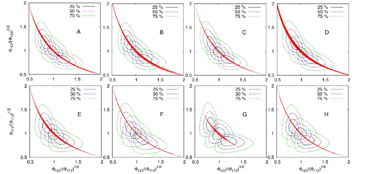
Figure 1: (Color online) 2D contours of constant joint probability density $\rho(X_{\bf r},Y_{\bf r})=\rho(\Phi_{23,{\bf r}}/(\Phi_{13,{\bf r}})^{1/2},\Phi_{12,{\bf r}}/(\Phi_{13,{\bf r}})^{1/2})$, computed using coarse graining boxes containing 125 particles on average. Each set of three concentric contours is chosen so that they enclose $25\%,50\%$ and $75\%$ of the total probability. Each panel from A to H contains results from the corresponding dataset, for $(X,Y)\approx(0.80,1.25),(1.00,1.00)$ and $(1.25,0.80)$, with the times chosen as late as possible within each dataset. The global values $(X(t_{1},t_{2},t_{3}),Y(t_{1},t_{2},t_{3}))$, for all times $t_{1}>t_{2}>t_{3}$ in each dataset, are shown with red points.

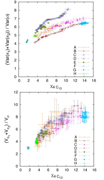
Figure 2: (Color online) Anisotropy ratios between transverse and longitudinal fluctuations, plotted as functions of $\chi_{4,C(t_{1},t_{3})}\equiv\chi_{4}(t_{1},t_{3})$ Toninelli2005 ; Parsaeian2008 , which measures the strength of the dynamical heterogeneity. Plotted for all datasets and all times consistent with $C(t_{1},t_{3})=0.23$ and $C(t_{1},t_{2})=C(t_{2},t_{3})$. Top panel: Ratio between the variances of the transverse and longitudinal fluctuations. Bottom panel: Ratio between the correlation volumes corr_vol of the transverse and longitudinal fluctuations.

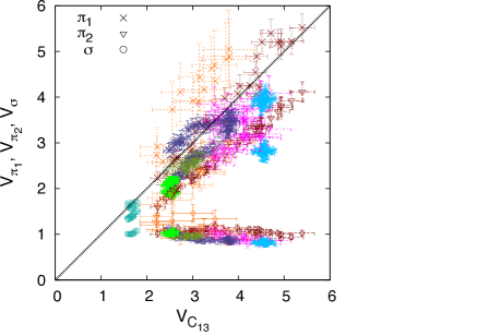
Figure 3: (Color online) Normalized correlation volumes $V_{\pi_{1}}$ (crosses), $V_{\pi_{2}}$ (triangles), and $V_{\sigma}$ (circles) for the transverse fluctuations ${\pi}_{1{\bf r}},{\pi}_{2{\bf r}}$ and the longitudinal fluctuations $\sigma_{\bf r}$, plotted as functions of the normalized correlation volume $V_{C_{13}}\equiv V_{C(t_{1},t_{3})}$ of the dynamical heterogeneities corr_vol . Plotted for all datasets and all times consistent with $C(t_{1},t_{3})=0.23$ and $C(t_{1},t_{2})=C(t_{2},t_{3})$. The color key for the datasets is as in Fig. 2.

To test the hypothesis given by Eq. (1), we will use the fact that for our data Bouchaud1997 :

$$C(t,t_{w})\approx f\left(h(t)/h(t_{w})\right),$$ (2)

where $f$ can be fitted with a form such that $C(t,t_{w})$ reduces to a stretched exponential in the equilibrium case: $f(x)=q_{EA}\exp\{-[\ln(x)/\theta_{0}]^{\beta}\}$ fit-parameters . Here $q_{EA}$, $\beta$ and $\theta_{0}$ are fitting parameters that vary little from one dataset to another. However, the dependence of the $\alpha$ relaxation time $\tau$ on $t_{w}$ is quite different in the different systems we consider triangular_long , and this leads to different forms for $h(t)$ Bouchaud1997 : for aging polymers $h(t)=\exp[\ln^{\alpha}(t/t_{0})]$, for aging particles $h(t)=\exp[(t/t_{0})^{\alpha}]$, and in equilibrium $h(t)=\exp(t/t_{0})$. We define $\Phi_{ab}\equiv f^{-1}\left[C(t_{a},t_{b})\right]$, with $a,b\in\{1,2,3\}$. If Eq. (2) is satisfied, we have $\Phi_{ab}\approx h(t_{a})/h(t_{b})$, and we therefore obtain a triangular relation Bouchaud1997 $\Phi_{13}\approx\Phi_{12}\Phi_{23}$. In terms of the variables $X\equiv\Phi_{23}/\sqrt{\Phi_{13}}$ and $Y\equiv\Phi_{12}/\sqrt{\Phi_{13}}$, this leads to the prediction that $1\approx XY$, which is satisfied to a good approximation for all times and all of our datasets triangular_long .

By using Eq. (2), we now re-express our hypothesis, Eq. (1), in the form $C_{\bf r}(t,t_{w})=f\left({h_{\bf r}(t)}/{h_{\bf r}(t_{w})}\right)$. We now define $\Phi_{ab,{\bf r}}\equiv f^{-1}\left[C_{\bf r}(t_{a},t_{b})\right]$, with $a,b\in\{1,2,3\}$, $X_{\bf r}(t_{1},t_{2},t_{3})\equiv\Phi_{23,{\bf r}}/\sqrt{\Phi_{13,{\bf r}}}$ and $Y_{\bf r}(t_{1},t_{2},t_{3})\equiv\Phi_{12,{\bf r}}/\sqrt{\Phi_{13,{\bf r}}}$, whose fluctuations also encode the properties of the dynamical heterogeneities. If the hypothesis in Eq. (1) is satisfied, then $1=X_{\bf r}Y_{\bf r}$, i.e., the relation holds locally not just globally. Since time reparametrization symmetry is a long time asymptotic effect associated with glassy behavior, we expect that as the temperature becomes lower, the timescales become longer, and the system becomes more glassy, the probability distribution $\rho(X_{\bf r},Y_{\bf r})$ should become anisotropic, and extend mostly in the direction of the global curve $1=XY$ and not away from it. In other words, if we decompose the fluctuations representing the dynamical heterogeneity into longitudinal and transverse variables Kardar2007 , the fluctuations of the longitudinal variable ${\sigma_{\bf r}}\equiv\frac{1}{\sqrt{3}}\ln(\Phi_{12,{\bf r}}\Phi_{23,{\bf r}}/\Phi_{13,{\bf r}})=\frac{1}{\sqrt{3}}\ln(X_{\bf r}Y_{\bf r})$ should become weaker than the fluctuations of the transverse variables ${\pi}_{1{\bf r}}\equiv\frac{1}{\sqrt{2}}\ln(\Phi_{12,{\bf r}}/\Phi_{23,{\bf r}})=\frac{1}{\sqrt{2}}\ln(Y_{\bf r}/X_{\bf r})$ and ${\pi}_{2{\bf r}}\equiv\frac{1}{\sqrt{6}}\ln(\Phi_{12,{\bf r}}\Phi_{23,{\bf r}}\Phi_{13,{\bf r}}^{2})$.

In Fig. (1) we show our results for $\rho(X_{\bf r},Y_{\bf r})$. Because we are trying to detect collective fluctuations, we coarse grain over moderately large regions, containing on average 125 particles. For each dataset, we find three triads of times $t_{1}>t_{2}>t_{3}$ such that $(X(t_{1},t_{2},t_{3}),Y(t_{1},t_{2},t_{3}))\approx(0.8,1.25),(1.00,1.00),$ and $(1.25,0.80)$ respectively. For each dataset and time triad, we show three contours of constant probability density $\rho(X_{\bf r},Y_{\bf r})$, respectively enclosing $25\%$, $50\%$ and $75\%$ of the total probability. For datasets A-D, with $T/T_{c}\sim 0.9$, the contours indeed follow the curve $1=XY$. This is more noticeable for the $25\%$ contour, which encloses the most likely fluctuations, than for the $50\%$ and $75\%$ contours, which additionally include rarer events. For datasets E and F, corresponding to $T/T_{c}=1.1$, the contours are still anisotropic and oriented along the direction of the global curve, but less so than in A-D, while for G and H, corresponding to $T/T_{c}=1.5$ the fluctuations away from the global curve are the strongest. For the higher temperatures, we find that the contours obtained in the aging regime (F, H) are similar to the ones obtained in the equilibrium regime (E, G) at the same temperatures Parsaeian2009 . These results can be directly connected to the fact that, as the temperature is increased, the separation of timescales is less pronounced, the finite time corrections to the time reparametrization symmetry become larger, and the effect of local time variable fluctuations become weaker.

We now turn to a more quantitative analysis of the connection between the transverse fluctuating variables $\pi_{1{\bf r}},\pi_{2{\bf r}}$, the longitudinal fluctuating variables $\sigma_{\bf r}$, and the dynamical heterogeneity. A more detailed version of this analysis will be presented elsewhere triangular_long . Here we report results for fixed $C(t_{1},t_{3})=0.23$, but similar results are obtained for other values of $C(t_{1},t_{3})$ triangular_long . In the top panel of Fig. (2) we show the ratio between the variances of the local transverse and longitudinal fluctuations as a function of $\chi_{4,C(t_{1},t_{3})}$ Toninelli2005 ; Parsaeian2008 ; corr_vol , which quantifies the strength of the dynamical heterogeneities. Similarly, in the bottom panel of Fig. (2) we plot the ratio between the correlation volumes corr_vol of transverse and longitudinal fluctuations as a function of $\chi_{4,C(t_{1},t_{3})}$. In both cases, we find that there is an anisotropy in favor of the transverse fluctuations, which grows as the strength of the dynamical heterogeneity increases. In particular, both ratios grow as the temperature is decreased, and in the case of systems in the aging regime, both ratios grow as the system relaxes, since $\chi_{4,C(t_{1},t_{3})}$ is a growing function of $t_{w}$ at fixed $C(t_{1},t_{3})$ Parsaeian2008 .

Our hypothesis is that the dynamical heterogeneity originates in the Goldstone modes associated to fluctuations in the time reparametrization, as described by Eq. (1). We thus expect that the correlation length of the dynamical heterogeneity should be similar to the correlation lengths of the transverse variables $\pi_{1}$ and $\pi_{2}$, and that the longitudinal variable $\sigma$ should be short-range correlated. In Fig. (3), we show that this is indeed the case: the normalized correlation volumes corr_vol $V_{\pi_{1}},V_{\pi_{2}}$ for the transverse fluctuations are approximately proportional to those for the dynamical heterogeneities, $V_{C_{13}}$, and in particular they grow as the temperature is reduced or as aging systems relax. By contrast, the normalized correlation volume for longitudinal fluctuations $V_{\sigma}$ is essentially constant for all systems, temperatures and time regimes, and approximately equal to unity, indicating that the spatial correlations of the variable $\sigma$ do not extend beyond the coarse graining region.

In conclusion, we have applied a stringent microscopic test for the hypothesis that dynamical heterogeneity in structural glasses is associated with the presence of spatially correlated fluctuations in the time variables, and we have found that all our results are consistent with this hypothesis. We have used data from molecular dynamics simulations of atomistic systems to apply the test, but the same procedure can be applied to particle tracking data from colloidal Weeks2000 and granular systems Keys2007 , and slight modifications would allow the study of light scattering Cipelletti2003 or dielectric noise Russell2000 data. This opens the door to investigating the possibility of a unified theoretical explanation of dynamical heterogenity for molecular liquids, colloidal liquids and granular systems. Our results highlight the advantages of studying dynamical heterogeneity by probing fluctuations of regions of the system, rather than probing individual particle fluctuations, since the latter will necessarily contain both collective and non-collective components that are difficult to separate cleanly. They also highlight the fact that more complex correlations in the time domain contain information that is useful for the understanding of heterogeneous dynamical behavior.

H. E. C. thanks L. Cugliandolo and C. Chamon for suggestions and discussions. This work was supported in part by DOE under grant DE-FG02-06ER46300, by NSF under grants PHY99-07949 and PHY05-51164, and by Ohio University. Numerical simulations were carried out at the Ohio Supercomputing Center. H. E. C. acknowledges the hospitality of the Aspen Center for Physics and the Kavli Institute for Theoretical Physics, where parts of this work were performed.

References

- (1) P. G. Debenedetti and F. H. Stillinger, Nature 410, 259 (2001).
- (2) M. D. Ediger, Annu. Rev. Phys. Chem. 51, 99 (2000).
- (3) W. Kob, C. Donati, S. J. Plimpton, P. H. Poole, and S. C. Glotzer, Phys. Rev. Lett. 79, 2827 (1997).
- (4) E. R. Weeks, J. C. Crocker, A. C. Levitt, A. B. Schofield, and D. A. Weitz, Science 287, 627 (2000).
- (5) E. Vidal Russell and N. E. Israeloff, Nature 408, 695 (2000).
- (6) C. Toninelli, M. Wyart, L. Berthier, G. Biroli, and J.-P. Bouchaud, Phys. Rev. E 71, 041505 (2005).
- (7) L. Cipelletti, H. Bissig, V. Trappe, P. Ballesta, and S. Mazoyer, J. Phys.: Condens. Matter 15, S257 (2003).
- (8) A. S. Keys, A. R. Abate, S. C. Glotzer, and D. J. Durian, Nature Physics 2007, 260–264, (2007).
- (9) J. P. Garrahan and D. Chandler, Phys. Rev. Lett. 89, 035704 (2002).
- (10) V. Lubchenko and P. G. Wolynes, Annu. Rev. Phys. Chem. 58, 235 (2007).
- (11) H. E. Castillo, C. Chamon, L. F. Cugliandolo, J. L. Iguain, and M. P. Kennett, Phys. Rev. B 68, 134442 (2003).
- (12) L. D. C. Jaubert, C. Chamon, L. F. Cugliandolo, and M. Picco, J. Stat. Mech. 2007, P05001, (2007).
- (13) C. Chamon, M. P. Kennett, H. E. Castillo, and L. F. Cugliandolo, Phys. Rev. Lett. 89, 217201 (2002).
- (14) H. E. Castillo, C. Chamon, L. F. Cugliandolo, and M. P. Kennett, Phys. Rev. Lett. 88, 237201 (2002).
- (15) H. E. Castillo and A. Parsaeian, Nature Physics 3, 26 (2007).
- (16) H. E. Castillo, Phys. Rev. B 78, 214430 (2008); G. A. Mavimbela and H. E. Castillo, J. Stat. Mech. 2011 P05017 (2011).
- (17) A. Parsaeian and H. E. Castillo, arXiv:0811.3190(2008).
- (18) A. Parsaeian and H. E. Castillo, Phys. Rev. E 78, 060105(R) (2008).
- (19) A. Parsaeian and H. E. Castillo, Phys. Rev. Lett. 102, 055704 (2009).
- (20) M. Kardar, Statistical Physics of Fields (Cambridge University Press, 2007).
- (21) L. Berthier and G. Tarjus, Phys. Rev. Lett 103, 170601 (2009).
- (22) W. Kob and J. L. Barrat, Phys. Rev. Lett. 78, 4581 (1997).
- (23) U. Bengtzelius, W. Götze, and A. Sjölander, J. Phys. C 17, 5915 (1984).
- (24) J.-P. Bouchaud, L. F. Cugliandolo, J. Kurchan, and M. Mézard, arXiv:condmat/9702070(1997).
- (25) The fitting parameters are reported at EPAPS.
- (26) K. E. Avila, H. E. Castillo, and A. Parsaeian, in preparation.
- (27) We estimate normalized correlation volumes by the formula , where , , is a local coarse grained variable, is the spatial average of , is the total volume of the system, is the coarse graining volume, and denotes an average over MD runs triangular_long .