Abstract

When Einstein formulated his special relativity in 1905, he established the law of Lorentz transformations for point particles. It is now known that particles have internal space-time structures. Particles, such as photons and electrons, have spin variables. Protons and other hadrons are regarded as bound states of more fundamental particles called quarks which have their internal variables. It is still one of the most outstanding problems whether these internal space-time variables are transformed according to Einstein’s law of Lorentz transformations. It is noted that Wigner, Dirac, and Feynman made important contributions to this problem. By integrating their efforts, it is then shown possible to construct a picture of the internal space-time symmetry consistent with Einstein’s Lorentz covariance.

1 Introduction

It took Issac Newton twenty years to extend his law of gravity from two particles to two extended objects, such as the sun and the earth. To do this, he had to develop a new mathematics now called integral calculus.

When Einstein formulated his special relativity in 1905, his transformation law was for point particles. We still do not know what happens to classical rigid bodies, but quantum mechanics allows us to replace those by standing waves. In the case of hydrogen atom, one can argue that the circular orbit appears as an ellipse to a moving observer [1], but not much has been done beyond this.

In quantum mechanics, the hydrogen atom is a localized probability distribution constructed from a standing wave solution of Schrödinger’s wave equation. We do not observe too often hydrogen atoms moving with relativistic speed, but relativistic-speed protons are abundantly produced from accelerators. Like the hydrogen atom, the proton is a bound state. The constituents are the quarks.

In 1939 [2], Eugene Wigner published a paper on the little groups of the Lorentz group whose transformations leave the four-momentum of a given particle invariant. He showed that the little groups for particles with non-zero mass are isomorphic to the three-dimensional rotation group. If the particle is at rest, this symmetry group is the three-dimensional rotation group. In this way, Wigner was able to define the particle’s spin as a space-time variable in the Lorentz covariant world. In 1939, composite particles, such as hadrons in the quark model, were unthinkable.

In a series of papers from 1927 to 1963, Paul A. M. Dirac attempted to construct a Lorentz-covariant picture of localized wave functions. In 1927 [3], he produced the concept of the c-number time-energy uncertainty relation and noted the basic space-time asymmetry. In 1945 [4], he considered the possibility of harmonic oscillators which can be Lorentz-transformed. In 1949 [5], he formulated the technique of light-cone variables to deal with Lorentz boosts. In 1963 [6], Dirac observed that two coupled oscillators can produce the symmetry of the Lorentz group of three space coordinates and two time variables.

In 1971 [7], Feynman et al. attempted to understand the hadronic mass spectra in terms of the degeneracies of the three-dimensional harmonic oscillator. In so doing they wrote down a harmonic oscillator differential equation which takes the same form for all Lorentz frames. This Lorentz-invariant differential equation has many different solutions, but they chose a set of solutions that violate all the rules of quantum mechanics and relativity. We show in this paper that their equation can have solutions which are consistent with the observations made earlier by both Wigner and Dirac.

In 1969 [8, 9], Feynman had observed that the ultra-fast proton can appear like a collections of partons while the proton is like a bound state of quarks. Since the partons have properties quite different those of the quarks, Feynman’s parton picture presents a nontrivial covariance problem. In 1905, Einstein had the problem of showing that the energy-momentum relation takes different forms for slow and fast particles.

In this paper, we review the efforts made by Wigner, Dirac, and Feynman in Secs. 2, 3, and 4 respectively. We then integrate their contributions in Sec. 5 to produce a Lorent-covariant picture of quantum bound states. Finally, in Sec. 6, we discuss experimental consequences of this covariant formalism.

2 Wigner’s Little Groups

In his 1939 [2], Wigner constructed subgroups of the Lorentz group whose transformations leave the four-momentum of a given particle invariant. They are called the little groups. The little groups are isomorphic to the $O(3)$ and to $O(2,1)$ groups if the particle momentum is time-like and space-like respectively. If the four-momentum is light-like, the little group is isomorphic to the two-dimensional Euclidean group. Since the momentum remains invariant, the little groups dictate the internal space-time symmetries of particles in the Lorentz-covariant world.

Since it is well known that the $SL(2,c)$ group serves as the covering group of the Lorentz group, it is possible to explain Wigner’s little groups in terms of two-by-two matrices. Let us consider the unimodular matrix

$$\pmatrix{A&B\cr C&D}$$ (1)

where all four elements are real numbers with $(AD-BC)=1.$ There are thus three independent parameters. This matrix can then be rotated to one of the following equi-diagonal matrices.

$$\pmatrix{\cos\theta&-e^{-\eta}\sin\theta\cr e^{\eta}\sin\theta&\cos\theta},\qquad\pmatrix{\cosh\lambda&e^{-\eta}\sinh\lambda\cr e^{\eta}\sinh\lambda&\cosh\lambda},\qquad\pmatrix{1&0\cr\gamma&1}.$$ (2)

This is purely a mathematical statement. However, they form the basis for Wigner’s little groups for massive particles, imaginary-mass particles, and massless particles respectively [10].

Let us look at the first matrix in Eq.(2). It can be written as

$$\pmatrix{e^{-\eta/2}&0\cr 0&e^{\eta/2}}\pmatrix{\cos\theta&\sin\theta\cr\sin\theta&\cos\theta}\pmatrix{e^{\eta/2}&0\cr 0&e^{-\eta/2}},$$ (3)

which corresponds to a Lorentz boost of the rotation matrix along the $z$ direction. The rotation matrix performs a rotation around the $y$ axis. The little group for the massive particle is a Lorentz-boosted rotation group.

Wigner noted in 1939 that, for a massive particle, there is a Lorentz frame where the particle is at rest. In this frame, rotations leave the particle four-momentum invariant, it can rotate internal space-time variables. The particle spin is the prime example. Wigner noted further that the third matrix of Eq.(2) corresponds to the little group for massless particles. Then there are two questions. The first question is what physical variable does $\gamma$ correspond to? The second question is whether this triangular matrix is a limiting case of the first matrix.

Let us answer the second question first. If the particle mass approaches zero, the $\eta$ parameter becomes infinitely large. If it is allowed to become large with $\theta e^{\eta/2}=\gamma,$ the angle $\theta$ has to become zero with $\cos\theta=1.$ The variable $\gamma$ is for the gauge transformation. These answers have a stormy history, but a geometric picture was developed by Kim and Wigner in 1990 [11]. Wigner’s little group is compared with Einstein’s energy-momentum relation in Table I.

Table I. Covariance of the energy-momentum relation, and covariance of the internal space-time symmetry groups.

Massive, Slow	COVARIANCE	Massless, Fast
$E=p^{2}/2m$	Einstein’s $E=mc^{2}$	$E=cp$
$S_{3}$		$S_{3}$
	Wigner’s Little Group
$S_{1},S_{2}$		Gauge Trans.

In 1939, it was unthinkable that the proton is a composite particle and is a bound state of the quarks. It can also move with a speed very close to that of light. In Sec. 4, we shall see whether this quantum bound state has the symmetry of Wigner’s little group using harmonic oscillators. This plan is illustrated in Fig. 1.

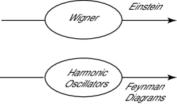
Figure 1: According to Einstein, point particles obey the Lorentz transformation law. We expect that the extended particles should obey the same law. Transformations of Wigner’s little groups leave the external momentum invariant, but change the internal space-time variables. In quantum field theory, Feynman diagrams describe running waves according to Einstein’s Lorentz covariance. It is possible to construct an oscillator-based model for internal space-time structure consistent with Wigner and thus with Einstein.

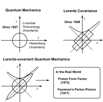
Figure 2: Space-time picture of quantum mechanics. In his 1927 paper, Dirac noted that there is a c-number time-energy uncertainty relation, in addition to Heisenberg’s position-momentum uncertainty relations, with quantum excitations. This idea is illustrated in the first figure (upper left). In his 1949 paper, Dirac produced his light-cone coordinate system as illustrated in the second figure (upper right). It is then not difficult to produce the third figure, for a Lorentz-covariant picture of quantum mechanics.

3 Dirac’s Attempts to make Quantum
Mechanics Lorentz Covariant

Paul A. M. Dirac made it his lifelong effort to make quantum mechanics consistent with special relativity. In 1927 [3], Dirac notes that there is an uncertainty relation between the time and energy variables which manifests itself in emission of photons from atoms. He notes further that there are no excitations along the time or energy axis, unlike Heisenberg’s uncertainty relation which allows quantum excitations. Thus, there is a serious difficulty in combining these relations in the Lorentz-covariant world.

In 1945 [4], Dirac considered a four-dimensional harmonic oscillator and attempted to construct a representation of the Lorentz group using the oscillator wave functions. However, he ends up with wave functions which do not appear to be Lorentz-covariant.

In 1949 [5], Dirac considered three forms of relativistic dynamics which can be constructed from the ten generators of the Poincaré group. He then imposed subsidiary conditions necessitated by the existing form of quantum mechanics. In so doing, he ends up with inconsistencies in all three of the cases he considers. On the other hand, he introduced the light-cone coordinate system which allows us to perform Lorentz boosts as squeeze transformations [12]

In 1963 [6], he constructed a representation of the $O(3,2)$ deSitter group using two harmonic oscillators. Using step-up and step-down operators, he constructs a beautiful algebra, but he made no attempt to exploit the physical contents of his algebra. Indeed, his representation now serves as the fundamental scientific language for squeezed states of light, further enforcing the point that Lorentz boosts are squeeze transformations [13].

We can combine Dirac’s time-energy uncertainty relations and his light-cone coordinate system to obtain a Lorentz-covariant picture of quantum mechanics, as shown in Fig. 2.

4 Feynman’s Phenomenological Equation for both Scattering and Bound States

In order to explain the hadron as a bound state of quarks, Feynman et al. start with two quarks whose space-time coordinates are $x^{a}_{\mu}$ and $x^{b}_{\mu}$ respectively [7] by using the equation

$$\left\{-\frac{1}{2}\left[\left(\frac{\partial}{\partial x^{a}_{\mu}}\right)^{2}+\left(\frac{\partial}{\partial x^{b}_{\mu}}\right)^{2}\right]+\frac{1}{16}\left(x^{a}_{\mu}-x^{b}_{\mu}\right)^{2}+m_{0}^{2}\right\}\phi\left(x^{a}_{\mu},x^{b}_{\mu}\right)=0.$$ (4)

If we use the hadronic and the quark separation coordinates as

$$X_{\mu}=\frac{1}{2}\left(x^{a}_{\mu}+x^{b}_{\mu}\right),\qquad x_{\mu}=\frac{1}{2\sqrt{2}}\left(x^{a}_{\mu}-x^{b}_{\mu}\right),$$ (5)

respectively, it is possible to consider the separation of the variables:

$$\phi\left(x^{a}_{\mu},x^{b}_{\mu}\right)=f\left(X_{\mu}\right)\psi\left(x_{\mu}\right).$$ (6)

Then the differential equation can be separated into the following two equations.

$$\left\{\left(\frac{\partial}{\partial X_{\mu}}\right)^{2}+m_{0}^{2}+(\lambda+1)\right\}f\left(X_{\mu}\right)=0$$ (7)

for the hadronic coordinate, and

$$\frac{1}{2}\left\{-\left(\frac{\partial}{\partial x_{\mu}}\right)^{2}+x_{\mu}^{2}\right\}\psi\left(x_{\mu}\right)=(\lambda+1)\psi\left(x_{\mu}\right),$$ (8)

for the coordinate of quarks inside the hadron.

The differential equation of Eq.(7) is a Klein-Gordon equation for the Lorentz-invariant hadronic coordinate. The differential equation of Eq.(4) contains the scattering-state equation for the hadron, and the bound-state equation for the quarks inside the hadron. Additionally, it is Lorentz-invariant.

However, in their paper [7], Feynman et al. did not consider whether their solutions are consistent with the symmetry of Wigner’s little group explained in Sec. 2 of the present paper. Let us now construct a representation of Wigner’s little group using the oscillator solutions. As noted earlier [14, 15], a set of solutions for the oscillator equation of Eq.(8) corresponds to a representation of Wigner’s $O(3)$-like little group for massive particles. If the hadron is at rest, its wave function should satisfy the $O(3)$ symmetry. We can achieve this goal by keeping the time-like oscillation in its ground state, and construct an $O(3)$-symmetric spatial wave function using the spherical coordinate system. We can then write the solution as

$$\psi(x,y,z,t)=\left[\left(\frac{1}{\pi}\right)^{1/4}\exp{\left(\frac{-t^{2}}{2}\right)}\right]\psi(x,y,z),$$ (9)

where the form of $\psi(x,y,z)$ in the spherical coordinate system is well known. This spherical solution can also be written as a linear combination of solutions in the Cartesian coordinate system, which take the form

$$\left[\frac{1}{\pi\sqrt{\pi}2^{(a+b+n)}a!b!n!}\right]^{1/2}H_{a}(x)H_{b}(y)H_{n}(z)\exp{\left\{-\left(\frac{x^{2}+y^{2}+z^{2}}{2}\right)\right\}},$$ (10)

where $H_{n}(z)$ is the Hermite polynomial.

It is now possible to boost this solution along the z direction. Since the transverse $x$ and $y$ coordinates are not affected by this boost, we can separate out these variables in the oscillator differential equation of Eq.(8), and consider the differential equation

$$\frac{1}{2}\left\{\left[-\left(\frac{\partial}{\partial z}\right)^{2}+z^{2}\right]-\left[-\left(\frac{\partial}{\partial t}\right)^{2}+t^{2}\right]\right\}\psi(z,t)=n\psi(z,t).$$ (11)

This differential equation remains invariant under the Lorentz boost

$$z^{\prime}=(\cosh\eta)z-(\sinh\eta)t,\qquad t^{\prime}=(\cosh\eta)t-(\sinh\eta)z,$$ (12)

where

$$e^{\eta}=\sqrt{\frac{1+\beta}{1-\beta}}$$

with $\beta=v/c$.

If we suppress the excitations along the $t$ coordinate, the normalized solution of this differential equation is

$$\psi(z,t)=\left(\frac{1}{\pi 2^{n}n!}\right)^{1/2}H_{n}(z)\exp{\left\{-\left(\frac{z^{2}+t^{2}}{2}\right)\right\}}.$$ (13)

We can boost this wave function by replacicing $z$ and $t$ by $z^{\prime}$ and $t^{\prime}$ of Eq.(12) respectively.

5 Lorentz-covariant Wave Functions with
Physical Interpretation

While the oscillator equation given in Eqs. (13) and (LABEL:sol55) of Sec. 4 are solutions of the equation of Feynman et al., we should exact meaningful physics from them. To do this we examine whether it is possible to construct localized quantum probability distributions. In terms of the light-cone variables defined in [5], Eqs. (13) and (LABEL:sol55) can be written as

$$\psi_{0}^{n}(x,t)=\left[\frac{1}{\pi n!2^{n}}\right]^{1/2}H_{n}\left(\frac{u+v}{\sqrt{2}}\right)\exp{\left\{-\left(\frac{u^{2}+v^{2}}{2}\right)\right\}},$$ (14)

and

$$\psi_{\eta}^{n}(x,t)=\left[\frac{1}{\pi n!2^{n}}\right]^{1/2}H_{n}\left(\frac{e^{-\eta}u+e^{\eta}v}{\sqrt{2}}\right)\exp{\left\{-\left(\frac{e^{-2\eta}u^{2}+e^{2\eta}v^{2}}{2}\right)\right\}},$$ (15)

for the rest and moving hadrons respectively. This form can be expanded as [15]

$$\psi_{\eta}^{n}(z,t)=\left(\frac{1}{\cosh\eta}\right)^{(n+1)}\sum_{k}\left[\frac{(n+k)!}{n!k!}\right]^{1/2}(\tanh\eta)^{k}\chi_{n+k}(z)\chi_{n}(t),$$ (16)

where $\chi_{n}(z)$ is the $n$-th excited state oscillator wave function which takes the familiar form

$$\chi_{n}(z)=\left[\frac{1}{\sqrt{\pi}2^{n}n!}\right]^{1/2}H_{n}(z)\exp{\left(\frac{-z^{2}}{2}\right)}.$$ (17)

If the hadron is at rest, there are no time-like oscillations, but for a moving hadron there are. This is the way in which the space and time variable mix covariantly and also provides a resolution of the space-time asymmetry pointed out by Dirac in his 1927 paper [3].

5.1 Probability Interpretations

The Lorentz-covariant solution given in Eq.(13) is totally self-consistent with the quantum probability interpretation. However, this requires an interpretation of oscillator excitations along the time-separation coordinate $t$[15, 16]. We shall study this in terms of two harmonic oscillators. Let us start with a two-oscillator system with the Hamiltonian of the form

$$H_{+}=\frac{1}{2}\left\{\left[-\left(\frac{\partial}{\partial x_{1}}\right)^{2}+x_{1}^{2}\right]+\left[-\left(\frac{\partial}{\partial x_{2}}\right)^{2}+x_{2}^{2}\right]\right\},$$ (18)

and the equation

$$H_{+}\psi\left(x_{1},x_{2}\right)=\left(n_{1}+n_{2}+1\right)\psi\left(x_{1},x_{2}\right).$$ (19)

This is the Schrödinger equation for the two-dimensional harmonic oscillator. The differential equation is separable in the $x_{1}$ and $x_{2}$ variables, and the wave function can be written

$$\psi\left(x_{1},x_{2}\right)=\chi_{n_{1}}\left(x_{1}\right)\chi_{n_{2}}\left(x_{2}\right),$$ (20)

where $\chi_{n}(z)$ is the $n^{th}$ excited-state oscillator wave function which takes the form

$$\chi_{n}(x)=\left[\frac{1}{\sqrt{\pi}2^{n}n!}\right]^{1/2}H_{n}(x)\exp{\left(\frac{-x^{2}}{2}\right)}.$$ (21)

Thus

$$\psi\left(x_{1},x_{2}\right)=\left[\frac{1}{\pi 2^{(n_{1}+n_{2})}n_{1}!n_{2}!}\right]^{1/2}H_{n_{1}}\left(x_{1}\right)H_{n_{2}}\left(x_{2}\right)\exp{\left[-\frac{1}{2}\left(x_{1}^{2}+x_{2}^{2}\right)\right]}.$$ (22)

If the system is in ground state with $n_{1}=n_{2}=0$, the above wave function becomes

$$\psi\left(x_{1},x_{2}\right)=\left[\frac{1}{\pi}\right]^{1/2}\exp{\left[-\frac{1}{2}\left(x_{1}^{2}+x_{2}^{2}\right)\right]}.$$ (23)

If only the $x_{2}$ coordinate is in its ground state, the wave function (with $n=n_{1}$) becomes

$$\psi\left(x_{1},x_{2}\right)=\left[\frac{1}{\pi 2^{n}n!}\right]^{1/2}H_{n}\left(x_{1}\right)\exp{\left[-\frac{1}{2}\left(x_{1}^{2}+x_{2}^{2}\right)\right]}.$$ (24)

If we introduce the normal coordinate system with

$$y_{1}=\frac{1}{\sqrt{2}}\left(x_{1}+x_{2}\right),\qquad y_{2}=\frac{1}{\sqrt{2}}\left(x_{1}-x_{2}\right),$$ (25)

and set

$$y_{1}\rightarrow e^{\eta}y_{1},\qquad y_{2}\rightarrow e^{-\eta}y_{1},$$ (26)

we can derive the equation[15, 13]

$$\psi_{\eta}^{n}\left(x_{1},x_{2}\right)=\left(\frac{1}{\cosh\eta}\right)^{(n+1)}\sum_{k}\left[\frac{(n+k)!}{n!k!}\right]^{1/2}(\tanh\eta)^{k}\chi_{n+k}\left(x_{1}\right)\chi_{n}\left(x_{2}\right).$$ (27)

This wave function is a linear combination of the eigen functions which satisfies the eigenvalue equation with the Hamiltonian $H_{-}$, where

$$H_{-}=\frac{1}{2}\left\{\left[-\left(\frac{\partial}{\partial x_{1}}\right)^{2}+x_{1}^{2}\right]-\left[-\left(\frac{\partial}{\partial x_{2}}\right)^{2}+x_{2}^{2}\right]\right\}.$$ (28)

Then

$$H_{-}\chi_{n}\left(x_{1}\right)\chi_{m}\left(x_{2}\right)=(n-m)\chi_{n}\left(x_{1}\right)\chi_{m}\left(x_{2}\right).$$ (29)

If the $x_{2}$ coordinate is in its ground state,

$$H_{-}\psi\left(x_{1},x_{2}\right)=n\psi\left(x_{1},x_{2}\right).$$ (30)

If we replace the notations $x_{1}$ and $x_{2}$ by $z$ and $t$ respectively, this Hamiltonian becomes that of Eq.(11).

5.2 Time-separation variable

We now understand the covariant harmonic oscillators in terms of the two coupled oscillators. In the case of the coupled oscillators, coordinates for both oscillators are well defined and carry their physical interpretation. However, in the covariant oscillators, the time-separation variable is still problematic.

This variable exists according to Einstein, and the differential equation of Eq.(8) is Lorentz-invariant because of this time-separation variable. Yet, its role has not been defined in the present form of quantum mechanics. On the other hand, it is possible to explain this variable in terms of Feynman’s rest of the universe [17, 18, 19]. The failure to observe this variable causes an increase in entropy and an additon of statistical uncertainty to the system.

6 Lorentz-covariant Quark Model

We started this paper with the Lorentz-invariant differential equation of Eq.(4). This phenomenological equation can explain the hadron spectra based on Regge trajectories and hadronic transition rates.

If we separate this equation using hadronic and quark variables, the equation can describe a hadron with a definite value for its four-momentum and its internal angular momentum. Furthermore, the hadronic mass is determined by the internal dynamics of the quarks. Our next question is whether these wave functions, particularly their Lorentz covariance properties, are consistent with what we observe in the real world.

The number of quarks inside a static proton is three, while Feynman observed that in a rapidly moving proton the number of partons appears to be infinite [9, 15]. The question then is how the proton looking like a bound state of quarks to one observer can appear different to an observer in a different Lorentz frame? Feynman made the following systematic observations:

• The picture is valid only for hadrons moving with velocity close to that of light.

• The interaction time between the quarks becomes dilated, and partons behave as free independent particles.

• The momentum distribution of partons becomes widespread as the hadron moves fast.

• The number of partons seems to be infinite or much larger than that of quarks.

Because the hadron is believed to be a bound state of two or three quarks, each of the above phenomena appears as a paradox, particularly b) and c) together. How can a free particle have a wide-spread momentum distribution? We have addressed this question extensively in the literature, and concluded that Gell-Mann’s quark model and Feynman’s parton model are two different manifestations of the same Lorentz-covariant quantity [15, 16, 20, 21, 22].

As for experimental observations of hadronic wave functions, it was noted by Hofstadter and McAllister in 1955 that the proton is not a point particle but has a space-time extension [23]. This discovery led to the study of electromagnetic form factor of the proton. As early as in 1970, Fujimura et al. calculated the electromagnetic form factor of the proton using the wave functions given in this paper and obtained the so-called “dipole” cut-off of the form factor [24].

In our 1973 paper [12], we attempted to explain the covariant oscillator wave function in terms of the coherence between the incoming signal and the width of the contracted wave function. This aspect was explained in the overlap of the energy-momentum wave function in our book [15]. Without this coherence, the form factor could decrease exponentially for increasing $(momentum~{}transfer)^{2}$. With this coherence, the decrease is slower and as shown experimentally, inversely proportional to the $(momentum~{}transfer)^{2}$.

Conclusions

The focal point of this paper is the Lorentz-invariant differential equation of Feynman et al. given in Sec. 4. This equation can be separated into the Klein-Gordon equation for the hadron and a harmonic-oscillator equation for the quarks inside the hadron.

From the solutions of this equation, it is possible to construct a representation of Wigner’s little group for massive particles. These solutions are consistent with both quantum mechanics and special relativity. Those oscillator solutions also explain Dirac’s efforts summarized in Fig. 2. In this way, we have combined the contributions made by Wigner, Dirac and Feynman to make quantum mechanics of bound states consistent with relativity.

We have also compared the covariant formalism with what we observe in high-energy physics, specifically the proton form factor and Feynman’s parton picture.

References

- [1] Bell, J. S. 2004 Speakable and Unspeakable in Quantum Mechanics, pp 71. Cambridge: Cambridge University Press.
- [2] Wigner, E. 1939 On Unitary Representations of the Inhomogeneous Lorentz Group. Ann. Math. 40, 149-204.
- [3] Dirac, P. A. M. 1927 The Quantum Theory of the Emission and Absorption of Radiation. Proc. Roy. Cocks. (London) A114, 243-265.
- [4] Dirac, P. A. M. 1945 Unitary Representations of the Lorentz Group. Proc. Roy. Cocci. (London) A183, 284-295.
- [5] Dirac, P. A. M. 1949 Forms of Relativistic Dynamics. Rev. Mod. Phys. 21, 392-399.
- [6] Dirac, P. A. M. 1963 A Remarkable Representation of the 3 + 2 de Sitter Group. J. Math. Phys. 4, 901-909.
- [7] Feynman, R. P., Kislinger, M. and Ravndal F. 1971 Current Matrix Elements from a Relativistic Quark Model. Phys. Rev. D 3, 2706-2732.
- [8] Feynman, R. P. 1969 Very High-Energy Collisions of Hadrons. Phys. Rev. Lett. 23, 1415-1417.
- [9] Feynman, R. P. 1969 The Behavior of Hadron Collisions at Extreme Energies in High Energy Collisions. In Proceedings of the Third International Conference, Stony Brook, NY (ed. C. N. Yang, et al.), pp 237-249. New York, NY: Gordon and Breach.
- [10] Kim, Y. S. 2010 Optical activities as computing resources for space-time symmetries. J. Mod. Optics 57, 17-22.
- [11] Kim, Y. S. and Wigner, E. P. 1990 Space-time geometry of relativistic particles. J. Math. Phys 31, 55-59.
- [12] Kim, Y. S., and Noz, M. E. 1973 Covariant harmonic oscillators and the quark model Phys. Rev. D 8, 3521-3627.
- [13] Kim, Y. S. and Noz, M. E. 1991 Phase Space Picture of Quantum Mechanics Singapore: World Scientific Publishing Company.
- [14] Kim, Y. S., Noz, M. E. and Oh, S. H. 1979 Representations of the Poincaré group for relativistic extended hadrons. J. Math. Phys.20, 1341-1344.
- [15] Kim, Y. S. and Noz, M. E. 1986 Theory and Applications of the Poincaré Group Dordrecht, The Netherlands: D. Reidel Publishing Company.
- [16] Kim, Y. S. and Noz, M. E. 1977 Covariant Harmonic Oscillators and the Parton Picture. Phys. Rev. D 15, 335-338.
- [17] Feynman, R. P. 1972 Statistical Mechanics, Reading, MA: Benjamin/Cummings.
- [18] Kim, Y. S. and Wigner, E. P. 1990 Entropy and Lorentz Transformations. Phys. Lett. A 147, 343-347.
- [19] Han, D., Kim, Y. S. & Noz, M. E. 1999 Illustrative Example of Feynman’s Rest of the Universe. Am. J. Phys. 67, 61-66.
- [20] Hussar, P. E. 1981 Valons and harmonic oscillators Phys. Rev. D 23, 2781-2783.
- [21] Kim, Y. S. 1989 Observable gauge transformations in the parton picture. Phys. Rev. Lett. 63, 348-351.
- [22] Kim, Y. S. and Noz, M. E. 2005 Coupled oscillators, entangled oscillators, and Lorentz-covariant harmonic oscillators. J. Opt. B: Quantum and Semiclass. Opt. 7, S458-S467.
- [23] Hofstadter, R. and McAllister, R. W. 1955 Electron Scattering from the Proton. Phys. Rev. 98, 217-218.
- [24] Fujimura, K., Kobayashi, T. and Namiki, M. 1970 Nucleon Electromagnetic Form Factors at High Momentum Transfers in an Extended Particle Model Based on the Quark Model. Prog. Theor. Phys. 43, 73-79.