Measurement of $C\!P$ observables in $B^{\pm}\rightarrow D_{C\!P}K^{\pm}$ decays and constraints on the CKM angle $\gamma$

Abstract

Using the entire sample of 467 million $\mathchar 28935\relax{(4S)}\rightarrow B\kern 1.79993pt\overline{\kern-1.79993ptB}{}$ decays collected with the BABAR detector at the PEP-II asymmetric-energy $B$ factory at SLAC, we perform an analysis of $B^{\pm}\rightarrow DK^{\pm}$ decays, using decay modes in which the neutral $D$ meson decays to either $C\!P$-eigenstates or non-$C\!P$-eigenstates. We measure the partial decay rate charge asymmetries for $C\!P$-even and $C\!P$-odd $D$ final states to be $A_{C\!P\!+}=0.25\pm 0.06\pm 0.02$ and $A_{C\!P\!-}=-0.09\pm 0.07\pm 0.02$, respectively, where the first error is the statistical and the second is the systematic uncertainty. The parameter $A_{C\!P\!+}$ is different from zero with a significance of 3.6 standard deviations, constituting evidence for direct $C\!P$ violation. We also measure the ratios of the charged-averaged $B$ partial decay rates in $C\!P$ and non-$C\!P$ decays, $R_{C\!P\!+}=1.18\pm 0.09\pm 0.05$ and $R_{C\!P\!-}=1.07\pm 0.08\pm 0.04$. We infer frequentist confidence intervals for the angle $\gamma$ of the unitarity triangle, for the strong phase difference $\delta_{B}$, and for the amplitude ratio $r_{B}$, which are related to the $B^{-}\rightarrow DK^{-}$ decay amplitude by $r_{B}e^{i(\delta_{B}-\gamma)}=A(B^{-}\rightarrow\kern 1.99997pt\overline{\kern-1.99997ptD}{}^{0}K^{-})/A(B^{-}\rightarrow D^{0}K^{-})$. Including statistical and systematic uncertainties, we obtain $0.24<r_{B}<0.45$ ($0.06<r_{B}<0.51$) and, modulo $180^{\circ}$, $11.3^{\circ}<\gamma<22.7^{\circ}$ or $80.8^{\circ}<\gamma<99.2^{\circ}$ or $157.3^{\circ}<\gamma<168.7^{\circ}$ ($7.0^{\circ}<\gamma<173.0^{\circ}$) at the 68% (95%) confidence level.

I Introduction

In the standard model (SM) of fundamental particles, $C\!P$ violation in weak interactions is allowed by a single, irreducible phase in the $3\times 3$ Cabibbo-Kobayashi-Maskawa (CKM) quark flavor-mixing matrix cabibbo ; ckmmatrix . The unitarity of the CKM matrix, $V$, implies a set of relations among its elements $V_{ij}$, in particular the condition $V_{ud}V_{ub}^{*}+V_{cd}V_{cb}^{*}+V_{td}V_{tb}^{*}=0$, which can be depicted in the complex plane as a “unitarity” triangle, whose sides and angles are related to the magnitudes and phases of the six elements $V_{id}$ and $V_{ib}$, where $i=u,c,t$. Overconstraining the unitarity triangle by means of precise measurements of all its sides and angles allows tests of whether the CKM mechanism is the correct description of $C\!P$ violation. Any inconsistencies among the various experimental constraints would reveal effects of physics beyond the standard model.

After a decade of successful operation and a total of about 1.3 billion $B\kern 1.79993pt\overline{\kern-1.79993ptB}{}$ pairs collected by the BABAR and Belle experiments, the three CKM angles have been measured with varied precision. The angle $\beta$ has been measured with the highest precision, to around $1^{\circ}$, using $B^{0}\rightarrow(c\bar{c})K^{(*)0}$ decays. Using a variety of two-body $B$ decays ($B\rightarrow\pi\pi,\ \rho\pi,\ \rho\rho$ and $a_{1}(1260)\pi$) the angle $\alpha$ has been measured to a precision of around $4^{\circ}$. The angle $\gamma$ has a relatively large uncertainty, around $14^{\circ}$, compared with $\alpha$ and $\beta$. The lack of precision in our knowledge of $\gamma$ reflects the difficulty in measuring this angle. The uncertainties of the CKM angles quoted in this paragraph are taken from CKMfitter .

Several techniques for measuring $\gamma$ in a theoretically clean way are based on $B$ meson decays to open-charm final states, $D^{(*)0}X_{s}$ and $\kern 1.99997pt\overline{\kern-1.99997ptD}{}^{(*)0}X_{s}$ ($X_{s}=K^{(*)\pm},\ K^{(*)0}$). In these decays, the interference between the $b\rightarrow c\bar{u}s$ and $b\rightarrow u\bar{c}s$ tree amplitudes, when the $D^{0}$ and $\kern 1.99997pt\overline{\kern-1.99997ptD}{}^{0}$ decay to a common final state, leads to observables that depend on the relative weak phase $\gamma$. The size of the interference also depends on the magnitude of the ratio $r_{B}$ and the relative phase strong phase $\delta_{B}$ of the two amplitudes, which can not be precisely calculated from theory. They can be extracted directly from data by simultaneously reconstructing several related $B\rightarrow DK$ decays. Many methods have been proposed to extract $\gamma$ from $B$ decays using $D^{(*)}K^{(*)\pm}$ and $D^{(*)}K^{(*)0}$ final states (here and in the following $D$ refers to any admixture of the neutral $D^{0}$ meson and its $C\!P$-conjugate $\kern 1.99997pt\overline{\kern-1.99997ptD}{}^{0}$). The three methods that have been used most productively to date are the “GLW” method GLW1 ; GLW2 , based on Cabibbo-suppressed $D$ decays to $C\!P$-eigenstates, such as $K^{+}K^{-}$ or $K^{0}_{S}\pi^{0}$; the “ADS” method ADS1 ; ADS2 , where the $D$ is reconstructed in Cabibbo-favored and doubly-Cabibbo-suppressed final states such as $K^{\pm}\pi^{\mp}$; and the “GGSZ” method DALITZ , which studies the Dalitz-plot distribution of the products of $D$ decays to multi-body self-conjugate final states, such as $K^{0}_{S}\pi^{+}\pi^{-}$. A common problem with these methods is the small overall branching fraction of these decays ranging from $5\times 10^{-6}$ to $5\times 10^{-9}$. Therefore a precise determination of $\gamma$ requires a very large data sample. BABAR has published several $\gamma$ related measurements: GLW analyses of $B^{\pm}\rightarrow DK^{\pm}$ babar_d0k_GLW_PRD , $D^{*}K^{\pm}$ babar_dstar0k_GLW_PRD and $DK^{*\pm}$ babar_d0kstar_GLWADS_PRD decays; ADS analyses of $B^{\pm}\rightarrow D^{(*)}K^{\pm}$ babar_dk_kpi_ADS_PRD ; babar_dk_kpipi0_ADS_PRD , $DK^{*\pm}$ babar_d0kstar_GLWADS_PRD and $B^{0}\rightarrow DK^{*0}$ babar_d0kstar0_ADS_PRD ; and GGSZ analyses of $B^{\pm}\rightarrow D^{(*)}K^{(*)\pm}$ babar_dk_DALITZ_PRD ; babar_dk_DALITZ_PRL and $B^{0}\rightarrow DK^{*0}$ decays babar_d0kstar0_DALITZ_PRD . To date, the single most precise experimental determination of $\gamma$ from BABAR is $\gamma=(68\pm 14\pm 4\pm 3)^{\circ}$ and $39^{\circ}<\gamma<98^{\circ}$, obtained from the GGSZ analysis of $B^{\pm}\rightarrow D^{(*)}K^{(*)\pm}$ decays babar_dk_DALITZ_PRL . In this measurement, the first error represents the statistical uncertainty, the second is the experimental systematic uncertainty, and the third reflects the uncertainty on the description of the $D$ Dalitz-plot distributions.

II GLW analysis of $B\rightarrow DK$ decays

In this paper we present the update of the GLW analysis of $B^{\pm}\rightarrow DK^{\pm}$ decays based on the full BABAR dataset collected near the $\mathchar 28935\relax{(4S)}$ resonance. In addition to a 22% increase in statistics of the data sample, this study benefits from other significant improvements compared to our previous result babar_d0k_GLW_PRD :

• More refined charged track reconstruction and particle identification algorithms, with higher purity and efficiency, have been employed;

• The event shape variable $\mathcal{F}$, used to discriminate the signal from the continuum $e^{+}e^{-}\rightarrow q\bar{q}$ background (described in detail in Section IV) has been removed from the selection criteria and has instead been included in the final fit to the selected $B$ candidates. This allows us to increase the signal efficiency by about 30%. At the same time it provides a larger sample of continuum background events, thus allowing for the determination of the background properties directly from data (see Section V);

• Better kaon/pion separation, which is needed to distinguish $B^{\pm}\rightarrow DK^{\pm}$ candidates from the twelve times more abundant $B^{\pm}\rightarrow D\pi^{\pm}$ decays, is achieved through the use of a global likelihood based not only on the Cherenkov angle $\theta_{C}$ reconstructed by the Cherenkov detector, but also on the specific energy loss ${\rm d}E/{\rm d}x$ measured by the tracking devices. The inclusion of ${\rm d}E/{\rm d}x$ in the likelihood increases the kaon identification efficiency and decreases the pion misidentification both at low momentum and outside of the geometrical acceptance of the Cherenkov detector (which is 10% lower than the acceptance of the tracking devices).

In order to determine $\gamma$ from $B^{\pm}\rightarrow DK^{\pm}$ decays with the GLW method, we measure the two direct-$C\!P$-violating partial decay rate asymmetries,

$$A_{C\!P\!\pm}\equiv\frac{\Gamma(B^{-}\rightarrow D_{C\!P\pm}K^{-})-\Gamma(B^{+}\rightarrow D_{C\!P\pm}K^{+})}{\Gamma(B^{-}\rightarrow D_{C\!P\pm}K^{-})+\Gamma(B^{+}\rightarrow D_{C\!P\pm}K^{+})}\,,$$ (1)

and the two ratios of charge averaged partial rates using $D$ decays to $C\!P$ and flavor eigenstates,

$$R_{C\!P\!\pm}\equiv 2\,\frac{\Gamma(B^{-}\rightarrow D_{C\!P\pm}K^{-})+\Gamma(B^{+}\rightarrow D_{C\!P\pm}K^{+})}{\Gamma(B^{-}\rightarrow D^{0}K^{-})+\Gamma(B^{+}\rightarrow\kern 1.99997pt\overline{\kern-1.99997ptD}{}^{0}K^{+})}\,,$$ (2)

where $D_{C\!P\!\pm}$ refer to the $C\!P$ eigenstates of the $D$ meson system. We then extract $\gamma$, together with the other two unknowns $r_{B}$ and $\delta_{B}$, by means of a frequentist procedure, which exploits the following relations GLW1 ; GLW2 , neglecting $D^{0}$–$\kern 1.99997pt\overline{\kern-1.99997ptD}{}^{0}$ mixing MIXING :

$$R_{C\!P\pm} = 1+r_{B}^{2}\pm 2r_{B}\cos\delta_{B}\cos\gamma\,,$$ (3)

$$A_{C\!P\pm} = \frac{\pm 2r_{B}\sin\delta_{B}\sin\gamma}{1+r_{B}^{2}\pm 2r_{B}\cos\delta_{B}\cos\gamma}.$$ (4)

Here, $r_{B}{\equiv}\left|A(B^{-}{\rightarrow}{\kern 1.99997pt\overline{\kern-1.99997ptD}{}^{0}}K^{-})/A(B^{-}{\rightarrow}{D^{0}}K^{-})\right|$ is the magnitude of the ratio of the amplitudes for $B^{-}{\rightarrow}{\kern 1.99997pt\overline{\kern-1.99997ptD}{}^{0}}K^{-}$ and $B^{-}{\rightarrow}{D^{0}}K^{-}$ and $\delta_{B}$ the difference of their strong phases. Taking into account the CKM factor ($|V_{ub}V_{cs}/V_{cb}V_{us}|\approx 0.4$) and color-suppression of the $B^{-}{\rightarrow}{\kern 1.99997pt\overline{\kern-1.99997ptD}{}^{0}}K^{-}$ amplitude, $r_{B}$ is expected to be around 0.1. The current world averages for the $B^{\pm}\rightarrow DK^{\pm}$ GLW observables from the measurements in babar_d0k_GLW_PRD ; belle_dk_GLW_PRD ; CDF_d0k_GLW are summarized in Table 1.

Table 1: World averages at 68% confidence level HFAG for the GLW observables in $B\rightarrow DK$ decays.

$C\!P$ of the $D$	$R_{C\!P}$	$A_{C\!P}$
$+1$	$1.10\pm 0.09$	$\phantom{-}0.24\pm 0.07$
$-1$	$1.06\pm 0.10$	$-0.10\pm 0.08$

The world averages for the parameters $r_{B}$ and $\delta_{B}$ are $r_{B}{=}0.104^{+0.015}_{-0.025}$ and $\delta_{B}{=}(117^{+17}_{-24})^{\circ}$ at 68% confidence level (CL) CKMfitter .

To reduce the systematic uncertainties from branching fractions and reconstruction efficiencies of different $D$ channels appearing in the numerator and denominator of Eq. 2, we approximate $R_{C\!P\!\pm}$ with the double ratios

$$R_{C\!P\pm}\approx\frac{R_{K/\pi}^{\pm}}{R_{K/\pi}}\ ,$$ (5)

where

$$R_{K/\pi}^{\pm}\equiv\frac{\Gamma(B^{-}\rightarrow D_{C\!P\pm}K^{-})+\Gamma(B^{+}\rightarrow D_{C\!P\pm}K^{+})}{\Gamma(B^{-}\rightarrow D_{C\!P\pm}\pi^{-})+\Gamma(B^{+}\rightarrow D_{C\!P\pm}\pi^{+})}\,,$$ (6)

and

$$R_{K/\pi}\equiv\frac{\Gamma(B^{-}\rightarrow D^{0}K^{-})+\Gamma(B^{+}\rightarrow\kern 1.99997pt\overline{\kern-1.99997ptD}{}^{0}K^{+})}{\Gamma(B^{-}\rightarrow D^{0}\pi^{-})+\Gamma(B^{+}\rightarrow\kern 1.99997pt\overline{\kern-1.99997ptD}{}^{0}\pi^{+})}\,.$$ (7)

Equation 5 would be exact in the limit in which the Cabibbo-suppressed contributions to the $B^{\pm}\rightarrow D\pi^{\pm}$ amplitudes vanish, as well as terms proportional to $r_{B}r_{D}\approx 5\times 10^{-3}$, as we will discuss in Section VII. This approximation results in a systematic uncertainty on the final values of $R_{C\!P\pm}$.

The paper is organized as follows. In Section III we describe the data sample used for these measurements and the main features of the BABAR detector and of the PEP-II storage rings. In Section IV we summarize the procedure adopted to select $B^{\pm}\rightarrow Dh^{\pm}$ candidates and suppress the main backgrounds. In Section V we introduce the simultaneous extended maximum likelihood fit used to extract the observables $R_{C\!P\!\pm}$ and $A_{C\!P\!\pm}$. In Section VI we explain how, by applying the same fit procedure to selected control samples, we estimate the irreducible background present in the final samples. A discussion of the sources of systematic uncertainties and the evaluation of the uncertainties is presented in Section VII. Section VIII lists the final results on the GLW observables $R_{C\!P\pm}$ and $A_{C\!P\pm}$, including statistical and systematic uncertainties. It also contains a description of the statistical method used to construct frequentist confidence intervals for the parameters $\gamma$, $\delta_{B}$, and $r_{B}$. Section IX gives a summary of our results.

III Data sample and Detector

The measurements presented in this paper use the entire $B\kern 1.79993pt\overline{\kern-1.79993ptB}{}$ data sample collected with the BABAR detector at the PEP-II asymmetric-energy $B$ factory at the SLAC National Accelerator Laboratory. The $B\kern 1.79993pt\overline{\kern-1.79993ptB}{}$ pairs are produced from the decays of $\mathchar 28935\relax{(4S)}$ mesons that originate in collisions of 9.0$\mathrm{\,Ge\kern-1.00006ptV}$ electrons and 3.1$\mathrm{\,Ge\kern-1.00006ptV}$ positrons ($\sqrt{s}{=}10.58\mathrm{\,Ge\kern-1.00006ptV}{=}M_{\mathchar 28935\relax{(4S)}}c^{2})$. In total, $(467\pm 5)\times 10^{6}$ $B\kern 1.79993pt\overline{\kern-1.79993ptB}{}$ pairs, approximately equally divided into $B^{0}\kern 1.79993pt\overline{\kern-1.79993ptB}{}^{0}$ and $B^{+}B^{-}$, have been collected in the years from 1999 until early 2008. The $B$ meson pairs are produced almost at rest in the $\mathchar 28935\relax{(4S)}$ center-of-mass (CM) frame, but the asymmetric beam energies boost them in the laboratory frame by $(\beta\gamma)_{\rm CM}\approx 0.56$.

The BABAR detector is described in detail elsewhere babar_detector . Primary and secondary vertex reconstruction and charged-particle tracking are provided by a five layer double-sided silicon vertex tracker and a 40 layer drift chamber. Charged particle identification (PID) is provided by measurement of specific ionization energy loss in the tracking devices and of the Cherenkov radiation cone in a ring-imaging detector. Photons and electrons are identified by combining the information from the tracking devices and the energy deposits in the electromagnetic calorimeter, which consists of 6580 thallium-doped CsI crystals. These systems are located inside a $1.5\,\textrm{T}$ solenoidal superconducting magnet. Finally, the flux return of the magnet is instrumented with resistive plate chambers and limited streamer tubes in order to discriminate muons from pions. We use the GEANT4 geant software toolkit to simulate interactions of particles in the detector, taking into account the varying accelerator and detector conditions.

IV Event Selection

We reconstruct $B^{\pm}\rightarrow Dh^{\pm}$ decays, where the charged track $h$ is either a kaon or a pion. Neutral $D$ mesons are reconstructed in the $C\!P$-even eigenstates $\pi^{-}\pi^{+}$ and $K^{-}K^{+}$ ($D_{C\!P\!+}$), in the $C\!P$-odd eigenstates $K^{0}_{\scriptscriptstyle S}\pi^{0}$, $K^{0}_{\scriptscriptstyle S}\phi$ and $K^{0}_{\scriptscriptstyle S}\omega$ ($D_{C\!P\!-}$), and in the non-$C\!P$-eigenstate $K^{-}\pi^{+}$ ($D^{0}$ from $B^{-}\rightarrow D^{0}h^{-}$) or $K^{+}\pi^{-}$ ($\kern 1.99997pt\overline{\kern-1.99997ptD}{}^{0}$ from $B^{+}\rightarrow\kern 1.99997pt\overline{\kern-1.99997ptD}{}^{0}h^{+}$). $C\!P$ violation in the $K^{0}$–$\kern 1.99997pt\overline{\kern-1.99997ptK}{}^{0}$ system is neglected, $i.e.$ the $K^{0}_{\scriptscriptstyle S}$ is assumed to be a pure $C\!P=+1$ eigenstate. The $D_{C\!P}$ daughters are reconstructed in the decay modes $K^{0}_{\scriptscriptstyle S}\rightarrow\pi^{+}\pi^{-}$, $\phi\rightarrow K^{+}K^{-}$ and $\omega\rightarrow\pi^{-}\pi^{+}\pi^{0}$.

We optimize all our event selection requirements by maximizing the significance of the expected $B^{\pm}\rightarrow DK^{\pm}$ signal yield, defined as $N_{\rm sig}/\sqrt{N_{\rm sig}+N_{\rm bkg}}$, where $N_{\rm sig}$ ($N_{\rm bkg}$) is the expected signal (background) yield. The optimization is done for each $D$ decay channel using simulated signal and background events, which are generated with the EVTGEN software package evtgen .

Neutral pions are reconstructed by combining pairs of photon candidates with energy deposits larger than 30$\mathrm{\,Me\kern-1.00006ptV}$ that are not matched to charged tracks and whose energy deposition profile is consistent with that expected from a photon. The photon pair invariant mass is required to differ from the nominal $\pi^{0}$ mass PDG2008 by less than 2.5 times its resolution ($\sigma\approx 6{\mathrm{\,Me\kern-1.00006ptV\!/}c^{2}}$) and the total $\pi^{0}$ energy in the laboratory frame must be greater than 240$\mathrm{\,Me\kern-1.00006ptV}$ for $D\rightarrow K^{0}_{\scriptscriptstyle S}\pi^{0}$ and 210$\mathrm{\,Me\kern-1.00006ptV}$ for $\omega\rightarrow\pi^{+}\pi^{-}\pi^{0}$.

Neutral kaons are reconstructed from pairs of oppositely charged tracks with invariant mass within $2.5\sigma$ ($\sigma\approx 2.1{\mathrm{\,Me\kern-1.00006ptV\!/}c^{2}}$) of the nominal $K^{0}_{\scriptscriptstyle S}$ mass PDG2008 . The ratio between the $K^{0}_{\scriptscriptstyle S}$ signed 3-dimensional flight length and its uncertainty, determined from the position of the $K^{0}_{\scriptscriptstyle S}$ and the $D$ decay vertices and the $K^{0}_{\scriptscriptstyle S}$ momentum direction, must be greater than 1.9, 2.0, and 2.2 for $D\rightarrow K^{0}_{\scriptscriptstyle S}\pi^{0}$, $D\rightarrow K^{0}_{\scriptscriptstyle S}\phi$, and $D\rightarrow K^{0}_{\scriptscriptstyle S}\omega$, respectively.

The $\phi$ candidates are reconstructed from pairs of oppositely charged tracks passing kaon identification criteria with typical kaon selection efficiency of $\approx 98\%$ and pion misidentification of $\approx 15\%$. The two tracks are assigned the kaon mass hypothesis and their invariant mass is required to be within $6.5{\mathrm{\,Me\kern-1.00006ptV\!/}c^{2}}$ of the nominal $\phi$ mass PDG2008 (the resolution is $\sigma=1.0{\mathrm{\,Me\kern-1.00006ptV\!/}c^{2}}$ and the natural width is $\Gamma_{\phi}=4.3\mathrm{\,Me\kern-1.00006ptV}$). We also require that the helicity angle $\theta_{H}$ between the flight direction of one of the two kaons and the $D$ flight direction, in the $\phi$ rest frame, satisfies the condition $|\cos\theta_{H}|>0.4$. This requirement exploits the fact that in $D\rightarrow K^{0}_{\scriptscriptstyle S}\phi$ decays the $\phi$ is produced in a longitudinally polarized state, thus $\cos\theta_{H}$ follows a $\cos^{2}\theta_{H}$ distribution, while in $\phi$ candidates not from $D\rightarrow K^{0}_{\scriptscriptstyle S}\phi$ decays, $\cos\theta_{H}$ is approximately uniformly distributed.

The $\omega$ candidates are reconstructed from $\pi^{+}\pi^{-}\pi^{0}$ combinations with invariant mass within $17{\mathrm{\,Me\kern-1.00006ptV\!/}c^{2}}$ ($2\Gamma_{\omega}$) of the nominal $\omega$ mass PDG2008 (the resolution is $\sigma=6.9{\mathrm{\,Me\kern-1.00006ptV\!/}c^{2}}$). The charged pion candidates are required to pass pion identification criteria with pion selection efficiency around 98% and kaon misidentification rate around 12%. To improve the $\omega$ momentum resolution, the invariant mass of the two photons forming the $\pi^{0}$ candidate is constrained to the nominal $\pi^{0}$ mass. We define $\theta_{N}$ as the angle between the normal to the $\omega$ decay plane and the $D$ momentum in the $\omega$ rest frame, and $\theta_{\pi\pi}$ as the angle between the flight direction of one of the three pions in the $\omega$ rest frame and the flight direction of one of the other two pions in the two-pion rest frame. The quantities $\cos\theta_{N}$ and $\cos\theta_{\pi\pi}$ follow $\cos^{2}\theta_{N}$ and $(1-\cos^{2}\theta_{\pi\pi})$ distributions, respectively, for the signal, and are almost uniformly distributed for wrongly reconstructed $\omega$ candidates. We require the product $\cos^{2}\theta_{N}\sin^{2}\theta_{\pi\pi}>0.046$.

Neutral $D$ candidates are formed from two-body combinations of $K^{\pm}$, $\pi^{\pm}$, $K^{0}_{\scriptscriptstyle S}$, $\pi^{0}$, $\phi$ and $\omega$ candidates consistent with one of the six $D$ decay channels under study. To improve the $D_{C\!P\!-}$ momentum resolution, the invariant masses of the $\pi^{0}$ and $K^{0}_{\scriptscriptstyle S}$ daughters are constrained to the nominal $\pi^{0}$ and $K^{0}_{\scriptscriptstyle S}$ masses. To suppress poorly reconstructed $D$ candidates and candidates from random combinations, we perform a geometric fit of the $D$ daughters to a common origin, and reject $D$ candidates for which the $\chi^{2}$ probability of the vertex fit is lower than 0.01%. The invariant mass of a $D$ candidate $M_{D}$ must be within a range that corresponds to slightly more than twice the $M_{D}$ resolution, which varies from about 6${\mathrm{\,Me\kern-1.00006ptV\!/}c^{2}}$ for the $K^{0}_{\scriptscriptstyle S}\phi$ channel to about 44${\mathrm{\,Me\kern-1.00006ptV\!/}c^{2}}$ for the $K^{0}_{\scriptscriptstyle S}\pi^{0}$ channel. We apply the following particle identification criteria to the charged daughters of the $D$ meson: in $D\rightarrow\pi^{+}\pi^{-}$, the two pion candidates must pass the same pion identification criteria adopted in the reconstruction of $\omega\rightarrow\pi^{-}\pi^{+}\pi^{0}$; in $D\rightarrow K^{+}\kern-1.60004ptK^{-}$, the two kaon candidates are required to pass tighter kaon identification criteria than those applied to the $\phi$ daughters (typical kaon selection efficiency around 94%, and pion misidentification rate around 6%); in $D\rightarrow K^{-}\pi^{+}$, the kaon candidate must pass the same kaon identification criteria required for the $\phi$ daughters. In order to reduce the large combinatorial background from random combinations of tracks and photons in $e^{+}e^{-}\rightarrow q\bar{q}$ events ($q=u,d,s,c$), we put requirements on the cosine of the $D$ decay angle, $|\cos\theta_{D}|$. We define $\theta_{D}$ as the angle between one of the $D$ daughters in the $D$ rest frame, and the direction of the $D$ meson in the $B$ rest frame. Due to angular momentum conservation we expect the distribution of $\cos\theta_{D}$ to be uniform for $B^{\pm}\rightarrow Dh^{\pm}$, $D\rightarrow\pi^{+}\pi^{-}$ and $D\rightarrow K^{0}_{\scriptscriptstyle S}\pi^{0}$ signal events, while for $q\overline{q}$ events the distribution is strongly peaked at $\pm 1$. We require $|\cos\theta_{D}|<0.74$ (0.99) for the $B^{\pm}\rightarrow Dh^{\pm}$, $D\rightarrow\pi^{+}\pi^{-}$ ($D\rightarrow K^{0}_{\scriptscriptstyle S}\pi^{0}$) channel.

The invariant mass distributions of the reconstructed $D$ candidates, after all the other selection criteria described in this section have been applied, are shown in Fig. 1.

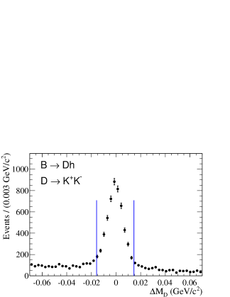
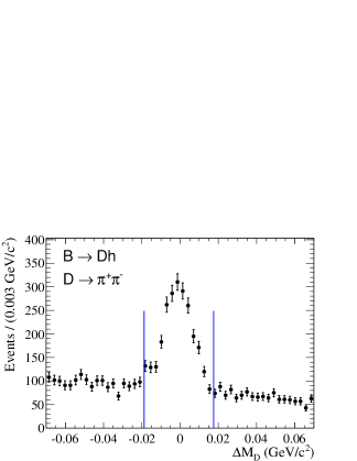
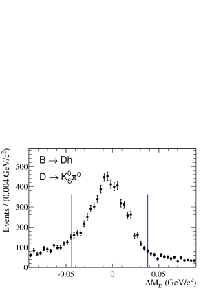
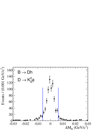
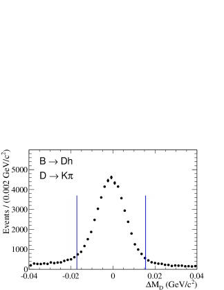
Figure 1: Distributions of the difference between the $D$ candidate’s invariant mass and the nominal $D^{0}$ mass PDG2008 , as measured in the $B^{\pm}\rightarrow Dh^{\pm}$ samples. All selection criteria described in Section IV, except that on the $D$ invariant mass $M_{D}$, have been applied, including the $\chi^{2}$-based candidate selection. In addition we reduce the background by requiring the fit variables to satisfy $\mbox{$m_{\rm ES}$}>5.27{\mathrm{\,Ge\kern-1.00006ptV\!/}c^{2}}$, $\mbox{$\Delta E$}>-0.05\mathrm{\,Ge\kern-1.00006ptV}$, and $\mathcal{F}>-0.25$. The $\Delta M_{D}$ selection requirements are depicted by the vertical lines.

We reconstruct $B^{\pm}$ meson candidates by combining a neutral $D$ candidate with a track $h^{\pm}$. For the $D{\rightarrow}K\pi$ mode, the charge of the track $h$ must match that of the kaon from the $D$ meson decay. This selects $b\rightarrow c$ mediated $B$ decays $B^{-}\rightarrow D^{0}h^{-}$ and $B^{+}\rightarrow\kern 1.99997pt\overline{\kern-1.99997ptD}{}^{0}h^{+}$. The contamination from $b\rightarrow u$ mediated $B$ decays followed by doubly-Cabibbo-suppressed $D$ decay, i.e. $B^{-}\rightarrow\kern 1.99997pt\overline{\kern-1.99997ptD}{}^{0}K^{-}$, $\kern 1.99997pt\overline{\kern-1.99997ptD}{}^{0}\rightarrow K^{-}\pi^{+}$, and from $D^{0}$–$\kern 1.99997pt\overline{\kern-1.99997ptD}{}^{0}$ mixing is negligible. In the $B^{\pm}\rightarrow Dh^{\pm}$, $D\rightarrow\pi^{+}\pi^{-}$ channel we require that the invariant mass of the $(h^{\pm}\pi^{\mp})$ system is greater than 1.9${\mathrm{\,Ge\kern-1.00006ptV\!/}c^{2}}$ to reject background from $B^{-}{\rightarrow}D^{0}\pi^{-}$, $D^{0}{\rightarrow}K^{-}\pi^{+}$ and $B^{-}{\rightarrow}K^{*0}\pi^{-}$, $K^{*0}{\rightarrow}K^{-}\pi^{+}$ decays and their $C\!P$ conjugates. Here $\pi$ is the pion from the $D$ and $h$ is the track from the $B$ candidate taken with the kaon mass hypothesis. To improve the $B$ momentum resolution, the neutral $D$ invariant mass is constrained to the nominal $D^{0}$ mass PDG2008 for all $D$ decay channels.

We identify signal $B\rightarrow DK$ and $B\rightarrow D\pi$ candidates using two kinematic variables: the difference between the CM energy of the $B$ meson ($E^{*}_{B}$) and the beam energy,

$$\Delta E=E^{*}_{B}-\sqrt{s}/2\ ,$$ (8)

and the beam-energy-substituted mass,

$$\mbox{$m_{\rm ES}$}=\sqrt{(s/2+\mathbf{p}_{ee}\cdot\mathbf{p}_{B})^{2}/E_{ee}^{2}-p_{B}^{2}},$$ (9)

where $(E_{B},\mathbf{p}_{B})$ and $(E_{ee},\mathbf{p}_{ee})$ are the four-momenta of the $B$ meson and of the initial $e^{+}e^{-}$ system, respectively, measured in the laboratory frame. The $m_{\rm ES}$ distributions for $B^{\pm}\rightarrow Dh^{\pm}$ signals are centered at the $B$ mass PDG2008 , have a root-mean-square of approximately 2.6${\mathrm{\,Me\kern-1.00006ptV\!/}c^{2}}$, and do not depend strongly on either the $D$ decay mode or the nature of the track $h$. In contrast, the $\Delta E$ distributions depend on the mass assigned to the track $h$. We evaluate $\Delta E$ with the kaon mass hypothesis so that the peaks of the distributions are centered near zero for $B^{\pm}\rightarrow DK^{\pm}$ events and are shifted by approximately $+50\mathrm{\,Me\kern-1.00006ptV}$ for $B^{\pm}\rightarrow D\pi^{\pm}$ events. The $\Delta E$ resolution depends on the kinematics of the decay, and is typically 16$\mathrm{\,Me\kern-1.00006ptV}$ for all $D$ decay modes under study after the $D$ invariant mass is constrained to its nominal value. We retain $B$ candidates with $m_{\rm ES}$ and $\Delta E$ within the intervals $5.20<\mbox{$m_{\rm ES}$}<5.29{\mathrm{\,Ge\kern-1.00006ptV\!/}c^{2}}$ and $-80<\mbox{$\Delta E$}<120\mathrm{\,Me\kern-1.00006ptV}$, which define the region for the fit described later.

In order to discriminate the signal from $e^{+}e^{-}\rightarrow q\bar{q}$ background events, denoted $q\bar{q}$ in the following, we construct a Fisher discriminant $\mathcal{F}$ based on the four event-shape quantities $L_{20}^{\rm ROE}$, $|\cos\theta_{T}^{*}|$, $|\cos\theta_{B}^{*}|$ and $H_{20}^{\rm ROE}$. These quantities, evaluated in the CM frame, are defined as:

• $L_{20}^{\rm ROE}=L_{2}/L_{0}$ is the ratio of the second and zeroth event shape moments of the energy flow in the rest of event (ROE), i.e. considering all the charged tracks and neutral clusters in the event that are not used to reconstruct the $B$ candidate. They are defined as $L_{2}=\sum_{i}p_{i}\cos^{2}\theta_{i}$ and $L_{0}=\sum_{i}p_{i}$, where $p_{i}$ are the momenta and $\theta_{i}$ the angles of the charged and neutral particles in the ROE, with respect to the thrust axis of the $B$ candidate’s decay products. The thrust axis is defined as the direction that maximizes the sum of the longitudinal momenta of the particles used to define it;

• $\theta_{T}^{*}$ is the angle between the thrust axis of the $B$ candidate’s decay products and the beam axis;

• $\theta_{B}^{*}$ is the angle between the $B$ candidate momentum and the beam axis;

• $H_{20}^{\rm ROE}=H_{2}/H_{0}$ is the ratio of the second and zeroth Fox-Wolfram moments $H_{2}$ and $H_{0}$ foxwolfram , computed using charged tracks and photons in the ROE.

The quantity $\mathcal{F}$ is a linear combination of the four aforementioned event-shape variables:

$$\mathcal{F}=c_{1}L_{20}^{\rm ROE}+c_{2}|\cos\theta_{T}^{*}|+c_{3}|\cos\theta_{B}^{*}|+c_{4}H_{20}^{\rm ROE}\,.$$ (10)

The values of the coefficients $c_{i}$ are the ones which maximize the separation between simulated signal events and a continuum background sample provided by off-resonance data, taken $\approx 40\mathrm{\,Me\kern-1.00006ptV}$ below the $\mathchar 28935\relax{(4S)}$ resonance. The maximum likelihood fit described in Section V is restricted to events with $\mathcal{F}$ within the interval $-1.5<\mathcal{F}<1.5$, to remove poorly reconstructed candidates.

For events with multiple $B^{\pm}\rightarrow Dh^{\pm}$ candidates (about 16% of the selected events), we choose the $B$ candidate with the smallest $\chi^{2}=\sum_{c}(M_{c}-M_{c}^{\rm PDG})^{2}/(\sigma^{2}_{M_{c}}+\Gamma^{2}_{c})$ formed from the measured and true masses, $M_{c}$ and $M_{c}^{\rm PDG}$, of all the unstable particles $c$ produced in the $B$ decay tree ($D$, $\pi^{0}$, $K^{0}_{\scriptscriptstyle S}$, $\phi$, $\omega$), scaled by the sum in quadrature of the resolution $\sigma_{M_{c}}$ of the reconstructed mass and the intrinsic width $\Gamma_{c}$. From simulated signal events, we find that this algorithm has a probability to select the correct candidate between 98.2% and 99.9% depending on the $D$ decay mode. We also find that the algorithm has negligible effect on the $M_{D}$ distributions.

We compare the distribution of each selection variable in data and simulated events after the requirements on all other variables have been applied. In order not to introduce biases that may artificially enhance the signal yield, we perform a blind study by explicitly removing, in this comparison, events consistent with the $B^{\pm}\rightarrow DK^{\pm}$ signal, $i.e.$ those with $|\mbox{$m_{\rm ES}$}-m_{B}|<10~{}{\mathrm{\,Me\kern-1.00006ptV\!/}c^{2}}$, $|\mbox{$\Delta E$}|<40~{}\mathrm{\,Me\kern-1.00006ptV}$, $\mathcal{F}>-0.8$ and track $h$ passing kaon identification criteria. We find excellent agreement between data and simulated events, both for events consistent with the $B^{\pm}\rightarrow D\pi^{\pm}$ signal ($|\mbox{$m_{\rm ES}$}-m_{B}|<10~{}{\mathrm{\,Me\kern-1.00006ptV\!/}c^{2}}$, $|\mbox{$\Delta E$}-50~{}\mathrm{\,Me\kern-1.00006ptV}|<40~{}\mathrm{\,Me\kern-1.00006ptV}$, $\mathcal{F}>-0.8$ and track $h$ failing the kaon identification criteria) and for background-like events. We correct for small differences in the means and widths of the distributions of the invariant masses of the unstable particles and of $m_{\rm ES}$ and $\Delta E$ both when applying to data the selection criteria obtained from simulated events and in the final fit described in the next section.

The total reconstruction efficiencies, based on simulated $B^{\pm}\rightarrow DK^{\pm}$ events, are summarized in the second column of Table 2.

Table 2: Reconstruction efficiency for $B\rightarrow DK$ from simulated events. We also quote the efficiency and purity in a signal-enriched subsample (see text for details).

$D^{0}$ mode	Efficiency after	Efficiency in	Purity in
	full selection	signal-enriched	signal-enriched
		subsample	subsample
$K^{-}\pi^{+}$	52%	22%	96%
$K^{+}\kern-1.60004ptK^{-}$	44%	18%	85%
$\pi^{+}\pi^{-}$	38%	17%	68%
$K^{0}_{\scriptscriptstyle S}\pi^{0}$	24%	10%	83%
$K^{0}_{\scriptscriptstyle S}\phi$	20%	9%	91%
$K^{0}_{\scriptscriptstyle S}\omega$	10%	4%	71%

For the reasons explained in Section II, the efficiencies are 40% to 60% higher than in our previous study of the same decay channels babar_d0k_GLW_PRD . The efficiencies obtained for $B^{\pm}\rightarrow D\pi^{\pm}$ events from the simulation are statistically consistent with those for $B^{\pm}\rightarrow DK^{\pm}$, where the $D$ meson is reconstructed in the same final state. For illustration purposes we define a signal-enriched sample for each $D$ decay mode, containing all $B^{\pm}\rightarrow Dh^{\pm}$ candidates satisfying the criteria $-40<\mbox{$\Delta E$}<100\mathrm{\,Me\kern-1.00006ptV}$, $0.2<\mathcal{F}<1.5$, $5.275<\mbox{$m_{\rm ES}$}<5.285{\mathrm{\,Ge\kern-1.00006ptV\!/}c^{2}}$, and whose daughter track $h$ passes charged kaon identification criteria. The typical kaon efficiency is $\approx 77\%$ and the pion misidentification rate is $\approx 2\%$. The reconstruction efficiencies and the expected purities for the signal-enriched subsamples, determined on simulated data, are listed in Table 2.

V Maximum Likelihood Fit

We measure $R_{K/\pi}^{(\pm)}$ and $A_{C\!P\!\pm}$ using simultaneous extended and unbinned maximum likelihood fits to the distributions of the three variables $\Delta E$, $m_{\rm ES}$, and $\mathcal{F}$ of $B$ candidates selected in data. The dataset is split into 24 subgroups by means of three discrete variables: the charge $\eta=\pm 1$ of the reconstructed $B$ meson ($\times$2 subgroups); the two-body $D$ decay final state $X$ ($\times 6$), allowing for a more accurate description of the corresponding probability density functions compared to the larger $C\!P\!\pm$ subgroups; and a PID variable denoting whether or not the track $h$ from the $B$ passes ($p$) or fails ($f$) charged kaon identification criteria ($\times 2$). The pion misidentification rate of these criteria is determined directly from data as described later, and is expected from simulation to be around 2%. The corresponding kaon identification efficiency is $(77\pm 1)\%$, as determined from the signal MC samples after weighting the bidimensional distribution of the momentum and polar angle of the track $h$ by the ratio of the analogous distributions observed in MC and data kaon control samples. The uncertainty on the kaon identification efficiency is dominated by the systematic contribution from the uncertainties on the weights. We perform in total three simultaneous fits to these 24 subgroups: one fit for the two $C\!P$-even $D$ final states (8 subgroups), one for the three $C\!P$-odd $D$ final states (12 subgroups), and one for the $D\rightarrow K\pi$ decay (4 subgroups).

The likelihood function $\mathcal{L}$ for each of these simultaneous fits has the form

$$\mathcal{L({\vec{\nu}})}=\frac{e^{-N}N^{n}}{n!}\prod_{s}\prod_{i=1}^{N_{s}}\mathcal{P}_{s}(m_{{\rm ES},i},\mbox{$\Delta E$}_{i},\mathcal{F}_{i};{\vec{\nu}}),$$ (11)

where $s$ ranges over the subgroups under consideration, $N_{s}$ is the number of events in subgroup $s$, $n$ is the total number of events in the fit $n=\sum_{s}N_{s}$, and $N$ is the expected number of events. We minimize $-\ln\mathcal{L}$ with respect to the set of fit parameters ${\vec{\nu}}$ specified later. The probability $\mathcal{P}_{s,i}\equiv\mathcal{P}_{s}(\mbox{$m_{\rm ES}$}_{i},\mbox{$\Delta E$}_{i},\mathcal{F}_{i})$ for an event $i$ is the sum of six signal and background components: $B^{\pm}\rightarrow DK^{\pm}$ signal, $B^{\pm}\rightarrow D\pi^{\pm}$ signal, background candidates from $e^{+}e^{-}\rightarrow q\overline{q}$ events, irreducible background arising from charmless $B^{\pm}\rightarrow XK^{\pm}$ and $B^{\pm}\rightarrow X\pi^{\pm}$ decays, and background candidates from other $B\kern 1.79993pt\overline{\kern-1.79993ptB}{}$ events (reducible $B\kern 1.79993pt\overline{\kern-1.79993ptB}{}$ background):

$$N_{s}\mathcal{P}_{s,i} = N_{s}^{D\pi}\mathcal{P}_{s,i}^{D\pi}+N_{s}^{DK}\mathcal{P}_{s,i}^{DK}+$$ (12)

$$N_{s}^{q\overline{q}}\mathcal{P}_{s,i}^{q\overline{q}}+N_{s}^{B\kern 1.25995pt\overline{\kern-1.25995ptB}{}}\mathcal{P}_{s,i}^{B\kern 1.25995pt\overline{\kern-1.25995ptB}{}}+$$

$$N_{s}^{X\pi}\mathcal{P}_{s,i}^{X\pi}+N_{s}^{XK}\mathcal{P}_{s,i}^{XK},$$

where the $N_{s}^{j}$ are the expected yields in each component $j$. In case of negligible correlations among the fit variables, each probability density function (PDF) $\mathcal{P}$ factorizes as:

$$\mathcal{P}(\mbox{$m_{\rm ES}$},\mbox{$\Delta E$},\mathcal{F})=\mathcal{P}(\mbox{$m_{\rm ES}$})\,\mathcal{P}(\mbox{$\Delta E$})\,\mathcal{P}(\mathcal{F}).$$ (13)

The irreducible $B\kern 1.79993pt\overline{\kern-1.79993ptB}{}$ background originates from events where a $B$ meson decays to the same final state $Xh$ as the signal, but without the production of an intermediate charmed meson in the decay chain. When exploiting the $\Delta E$, $m_{\rm ES}$, and $\mathcal{F}$ variables, this background is therefore indistinguishable from the signal. As an example, the decay $B^{\pm}\rightarrow K^{+}K^{-}K^{\pm}$ ($X=K^{+}\kern-1.60004ptK^{-}$) is an irreducible background for $B^{\pm}\rightarrow D_{C\!P+}K^{\pm}$, $D_{C\!P+}\rightarrow K^{+}\kern-1.60004ptK^{-}$. As described later in Section VI, the irreducible background yield can be estimated by studying sideband regions of the $D$ candidate invariant mass distribution, and can then be fixed in the final fit, where we assume $\mathcal{P}_{i}^{Dh}=\mathcal{P}_{i}^{Xh}$.

We express the signal yield parameters $N^{DK}_{s}$ and $N^{D\pi}_{s}$ through the $C\!P$ asymmetries $A^{X}_{DK}$ and $A^{X}_{D\pi}$ of $B^{\pm}\rightarrow DK^{\pm}$, $D{\rightarrow}X$ and $B^{\pm}\rightarrow D\pi^{\pm}$, $D{\rightarrow}X$, their branching fraction ratios, $R_{K/\pi}^{X}$, the total number $N^{D\pi}_{{\rm tot},X}$ of $B^{\pm}\rightarrow D\pi^{\pm}$, $D\rightarrow X$ signal events, the true kaon identification efficiency $\varepsilon$ of the PID selector, and the pion misidentification rate $m$ of the PID selector:

$$N^{DK}_{\eta,p,X} = \frac{1}{2}\left(1-\eta A^{X}_{DK}\right)\>N^{D\pi}_{{\rm tot},X}\>R_{K/\pi}^{X}\,\varepsilon\,,$$ (14)

$$N^{DK}_{\eta,f,X} = \frac{1}{2}\left(1-\eta A^{X}_{DK}\right)\>N^{D\pi}_{{\rm tot},X}\>R_{K/\pi}^{X}\,(1-\varepsilon)\,,$$ (15)

$$N^{D\pi}_{\eta,p,X} = \frac{1}{2}\left(1-\eta A^{X}_{D\pi}\right)\>N^{D\pi}_{{\rm tot},X}\>m\,,$$ (16)

$$N^{D\pi}_{\eta,f,X} = \frac{1}{2}\left(1-\eta A^{X}_{D\pi}\right)\>N^{D\pi}_{{\rm tot},X}\>(1-m)\,.$$ (17)

Because the ratios $R_{K/\pi}^{X}$ are small, the fit is not able to determine the value of $\varepsilon$. Therefore we fix it to the aforementioned value of $\varepsilon=(77\pm 1)\%$. The reconstruction and selection efficiencies for true $B^{\pm}\rightarrow DK^{\pm}$ and $B^{\pm}\rightarrow D\pi^{\pm}$ candidates, where the $D$ meson decays to the same final state, are assumed to be identical. A systematic uncertainty is assigned due to this assumption (see Section VII). The simultaneous fit to the two $C\!P$-even modes constrains

$$A^{\pi^{+}\pi^{-}}_{DK} = A^{K^{+}\kern-1.12003ptK^{-}}_{DK}\equiv A_{C\!P\!+}\,,$$ (18)

$$R_{K/\pi}^{\pi^{+}\pi^{-}} = R_{K/\pi}^{K^{+}\kern-1.12003ptK^{-}}\equiv R_{K/\pi}^{+}\,,$$ (19)

while the simultaneous fit to the three $C\!P$-odd modes constrains

$$A^{K^{0}_{\scriptscriptstyle S}\pi^{0}}_{DK} = A^{K^{0}_{\scriptscriptstyle S}\phi}_{DK}=A^{K^{0}_{\scriptscriptstyle S}\omega}_{DK}\equiv A_{C\!P\!-}\,,$$ (20)

$$R_{K/\pi}^{K^{0}_{\scriptscriptstyle S}\pi^{0}} = R_{K/\pi}^{K^{0}_{\scriptscriptstyle S}\phi}=R_{K/\pi}^{K^{0}_{\scriptscriptstyle S}\omega}\equiv R_{K/\pi}^{-}\,.$$ (21)

The $m_{\rm ES}$ distributions of the signal components are parameterized using an asymmetric Gaussian shape, i.e. a Gaussian with different widths on both sides of the peak. We use the same shape for $B^{\pm}\rightarrow DK^{\pm}$ and $B^{\pm}\rightarrow D\pi^{\pm}$, so the $m_{\rm ES}$ $B^{\pm}\rightarrow DK^{\pm}$ signal shape (whose parameters are floating in the fit) will mostly be determined by the much more abundant $B^{\pm}\rightarrow D\pi^{\pm}$ control sample. Since the selection efficiencies for the two channels are the same, we expect the number of reconstructed candidates from $B^{\pm}\rightarrow D\pi^{\pm}$ to be about twelve times higher than for $B^{\pm}\rightarrow DK^{\pm}$. We have checked that the $m_{\rm ES}$ shapes for $B^{\pm}\rightarrow DK^{\pm}$ and $B^{\pm}\rightarrow D\pi^{\pm}$ are consistent, and that the assumption that they are identical does not bias the parameters of interest.

The $\Delta E$ distribution of the $B^{\pm}\rightarrow DK^{\pm}$ signal component is parameterized with a double Gaussian shape. The core Gaussian has a mean close to zero, a width around 16$\mathrm{\,Me\kern-1.00006ptV}$ and, according to the simulation, accounts for about 90% of the true $B^{\pm}\rightarrow DK^{\pm}$ candidates. The second Gaussian accounts for the remaining 10% of candidates whose energy has been poorly measured. The mean and width of the core Gaussian are directly determined from data, while the remaining three parameters (the difference between the two means, the ratio between the two widths and the ratio of the integrals of the two Gaussian functions) are fixed from the simulation. In contrast to the $m_{\rm ES}$ case, the $B^{\pm}\rightarrow D\pi^{\pm}$ $\Delta E$ shape is not the same as for $B^{\pm}\rightarrow DK^{\pm}$. This is due to the fact that we always assign the kaon mass hypothesis to the track: the wrong mass assignment, in the case of $B^{\pm}\rightarrow D\pi^{\pm}$, introduces a shift to the reconstructed energy of the pion and thus to $\Delta E$, since $\mbox{$\Delta E$}=E^{*}_{B}-\sqrt{s}/2=E^{*}_{D}+E^{*}_{h}-\sqrt{s}/2$. The shift depends on the magnitude of the momentum ${\bf p}$ of the track $h$ in the laboratory frame,

$$\mbox{$\Delta E$}_{\tt shift}({\bf p})=\gamma_{\textrm{\small CM}}\left(\sqrt{m_{K}^{2}+{\bf p}^{2}}-\sqrt{m_{\pi}^{2}+{\bf p}^{2}}\right).$$ (22)

Therefore we parameterize the $B^{\pm}\rightarrow D\pi^{\pm}$ $\Delta E$ signal component with the sum of two Gaussians whose means are computed event-per-event by adding $\mbox{$\Delta E$}_{\tt shift}({\bf p})$ to the means of the Gaussian functions used to describe the $B^{\pm}\rightarrow DK^{\pm}$ $\Delta E$ signal. The other parameters of the $B^{\pm}\rightarrow D\pi^{\pm}$ and $B^{\pm}\rightarrow DK^{\pm}$ $\Delta E$ distributions (the two widths and the ratio of the integrals) are identical. Again, we exploit the $B^{\pm}\rightarrow D\pi^{\pm}$ control sample to determine the shape of the $B^{\pm}\rightarrow DK^{\pm}$ signal. In the case of the high statistics flavor mode $D\rightarrow K\pi$, we add a linear background component to the double Gaussian shape to account for misreconstructed events, which peak in $m_{\rm ES}$ but not in $\Delta E$. The ratio between the integral of the linear component and that of the two Gaussian functions is fixed from simulated signal events.

For the reducible $B\kern 1.79993pt\overline{\kern-1.79993ptB}{}$ background, Eq. 13 does not hold because of significant correlations between the $\Delta E$ and $m_{\rm ES}$ distributions. This reflects the fact that this background is composed of two categories of $B$ candidates with different $m_{\rm ES}$ and $\Delta E$ distribution:

• $B$ candidates formed from random combinations of charged tracks and neutral objects in the event, which populate the whole $m_{\rm ES}$-$\Delta E$ plane;

• $B$ candidates from $B^{\pm}\rightarrow D\rho^{\pm}$, $B^{\pm}\rightarrow DK^{*\pm}$, $B^{\pm}\rightarrow D^{*}h^{\pm}$ $(D^{*}\rightarrow D\pi)$, where a pion from the $\rho$, $K^{*}$ or $D^{*}$ decay is not reconstructed. These candidates peak in $m_{\rm ES}$ close to the $B$ mass, but with broader resolution compared to the signal, and are shifted towards negative $\Delta E$ values, typically peaking at $\mbox{$\Delta E$}\approx-m_{\pi}c^{2}$, therefore outside of the $\Delta E$ fit region; however, the tail on the positive side of the distribution extends into the $\Delta E$ fit region.

We parametrize the $m_{\rm ES}$-$\Delta E$ distribution of the $B\kern 1.79993pt\overline{\kern-1.79993ptB}{}$ background by means of two factorizing components:

$$\mathcal{P}_{B\kern 1.25995pt\overline{\kern-1.25995ptB}{}}(\mbox{$m_{\rm ES}$},\mbox{$\Delta E$})=f \times g_{\rm peak}(\mbox{$m_{\rm ES}$})h_{\rm peak}(\mbox{$\Delta E$})+$$

$$(1-f) \times g_{\rm cont}(\mbox{$m_{\rm ES}$})h_{\rm cont}(\mbox{$\Delta E$}).$$ (23)

The $m_{\rm ES}$ component of the peaking part, $g_{\rm peak}(\mbox{$m_{\rm ES}$})$, is parameterized with a Gaussian function for $X=\pi^{+}\pi^{-},\ K^{0}_{\scriptscriptstyle S}\omega,\ K^{0}_{\scriptscriptstyle S}\phi$. For $X=K^{+}\kern-1.60004ptK^{-},\ K^{0}_{\scriptscriptstyle S}\pi^{0}$ we use the “Crystal Ball” lineshape crystalball , an empirical smooth function that better describes the non-Gaussian tail on the negative side of the distribution,

$$C(x)=\left\{\begin{array}[]{ll}\frac{n^{n}}{|\alpha|^{n}}e^{-\frac{|\alpha|^{2}}{2}}\left(\frac{n}{|\alpha|}-|\alpha|-\bar{x}\right)^{-n}&\bar{x}<-|\alpha|\,,\\ \exp\left(-\frac{1}{2}\bar{x}^{2}\right)&\bar{x}\geq-|\alpha|\,,\end{array}\right.$$ (24)

with $\bar{x}=(x-\mu)/\sigma$ and $\bar{x}\rightarrow-\bar{x}$ for $\alpha<0$. For $X=K\pi$ we use an empirical function of the form:

$$N(x)=\exp\left(-\frac{1}{2\tau^{2}}\,\left\{\ln^{2}[1+\mathchar 28931\relax\tau(x-\mu)]+\tau^{4}\right\}\right)\,,$$ (25)

with $\mathchar 28931\relax=\sinh(\tau\sqrt{\ln 4})/(\sigma\tau\sqrt{\ln 4})$. Here $\mu$ is the position of the peak, while $\sigma$ and $\tau$ are parameters related to the width of the distribution on the two sides of the peak. The $\Delta E$ component of the peaking part $h_{\rm peak}(\mbox{$\Delta E$})$ is described with a simple exponential function for the five $C\!P$ self-conjugate $D$ final states, and with a Landau function for the non-$C\!P$-eigenstate final state. The $B\kern 1.79993pt\overline{\kern-1.79993ptB}{}$ purely combinatorial background component is described by the 2-dimensional product of a linear background, $h_{\rm cont}(\mbox{$\Delta E$})$, and an empirical function introduced by the ARGUS collaboration argus , $g_{\rm cont}(\mbox{$m_{\rm ES}$})=A(\mbox{$m_{\rm ES}$}/m_{0})$:

$$A(x)=x(1-x^{2})^{p}\exp\left(-\zeta\left[1-x^{2}\right]\right)\ ,$$ (26)

where $m_{0}=\sqrt{s}/(2c^{2})=5.29{\mathrm{\,Ge\kern-1.00006ptV\!/}c^{2}}$ is the kinematic endpoint of the $m_{\rm ES}$ distribution. All the parameters of the $B\kern 1.79993pt\overline{\kern-1.79993ptB}{}$ background $m_{\rm ES}$-$\Delta E$ distribution are fixed from simulated $B\kern 1.79993pt\overline{\kern-1.79993ptB}{}$ events. The only exception is the width of the Landau function used for $h_{\rm peak}(\mbox{$\Delta E$})$ in $X=K^{-}\pi^{+}$. This parameter controls the behaviour at low $\Delta E$ values, $\mbox{$\Delta E$}\approx-80\mathrm{\,Me\kern-1.00006ptV}$, where we find the simulation not to be sufficiently precise given the high statistics of this channel. We note that the shape parameters differ across the six final states, but are similar across the charge and PID selector subgroups belonging to one final state.

In $q\overline{q}$ events, $B$ candidates arise from random combinations of charged tracks and neutral particles produced in the hadronization of the light quark-antiquark pairs produced in $e^{+}e^{-}$ collisions. Similarly to the combinatorial component of the $B\kern 1.79993pt\overline{\kern-1.79993ptB}{}$ background, the $q\overline{q}$ background distribution in the $m_{\rm ES}$-$\Delta E$ plane is parameterized by the product of an ARGUS function in $m_{\rm ES}$ and a linear background in $\Delta E$. We float the slope of the linear components, while the parameters of the ARGUS function are fixed, in each $D$ final state, from simulated $q\overline{q}$ events. They are in good agreement across the final states and other subgroups.

The $\mathcal{F}$ distributions are parameterized in a similar way for all fit components. We find that the distributions of $B^{\pm}\rightarrow DK^{\pm}$ and $B^{\pm}\rightarrow D\pi^{\pm}$ signal events are consistent with each other, as expected since their kinematics are very similar, and choose to parameterize them with the same shape. For this we use the sum of two asymmetric Gaussian functions. Some channels with lower statistics don’t require the full complexity of this parameterization: in those cases we use a single asymmetric Gaussian, a double Gaussian, or a single Gaussian. In particular we use: for the signal components a double asymmetric Gaussian, except for $X=K^{0}_{\scriptscriptstyle S}\phi$, where a double Gaussian function is adopted; for the $B\kern 1.79993pt\overline{\kern-1.79993ptB}{}$ background components a double asymmetric Gaussian in case of $X=K^{0}_{\scriptscriptstyle S}\pi^{0},K^{-}\pi^{+}$, a double Gaussian in case of $X=K^{0}_{\scriptscriptstyle S}\omega$, and a single Gaussian otherwise; for the $q\overline{q}$ background components a double asymmetric Gaussian, except for $X=K^{0}_{\scriptscriptstyle S}\phi$, where we use a single Gaussian.

In summary, the floating parameters of the fits are: all parameters related to the signal yields, and therefore to the GLW parameters, as given in Eqns. 14-17, except $\varepsilon$; all background yields and $C\!P$-asymmetries except the irreducible background yields and asymmetries, the $B\kern 1.79993pt\overline{\kern-1.79993ptB}{}$ asymmetries for $C\!P\!-$ modes and for the $(C\!P\!+,p)$ subgroups ($B\rightarrow D_{C\!P+}h$ candidates where the track $h$ passes the kaon identification criteria), and the $B\kern 1.79993pt\overline{\kern-1.79993ptB}{}$ yield in the $(K^{0}_{\scriptscriptstyle S}\phi,p)$ subgroup; selected shape parameters, namely the overall width and mean of the $\Delta E$ signal, the $m_{\rm ES}$ signal shape, and the $\Delta E$ and $\mathcal{F}$ shape for $q\overline{q}$ background. A full list of the floating parameters can be found in Table 8. The non-floating parameters are fixed to their expectations obtained from simulation or, in case of the irreducible background yields, to values obtained from data control samples (see next section). Non-floating $C\!P$ asymmetries are fixed to zero. We assign systematic uncertainties due to the fixed parameters.

We check that the fitter is correctly implemented by generating and fitting a large number of test datasets using the final PDFs. In this study, we include an analytic description for the conditional variable $\mbox{$\Delta E$}_{\tt shift}$. The residuals for a given parameter, divided by the measured parameter error, should follow a Gaussian distribution with zero mean ($\mu$) and unitary width ($\sigma$). We observe no significant deviations from the expected distribution. In particular, $R_{K/\pi}^{+}$ shows the largest shift from zero mean ($\mu=-0.06\pm 0.07$) and $A_{C\!P\!+}$ shows the largest deviation from unity width ($\sigma=1.13\pm 0.06$) among the parameters of interest.

We investigate fit biases, arising from possible discrepancies between the true signal distribution and the chosen fit model, by fitting a large number of test datasets, in which the $B^{\pm}\rightarrow DK^{\pm}$ and $B^{\pm}\rightarrow D\pi^{\pm}$ signal components are taken from simulated samples of sufficient statistics, while the background components are randomly generated according to their PDFs. Of all floating parameters, only $R_{K/\pi}$ acquires a significant bias, resulting in corrections of 0.5 and 1.0 times the expected statistical uncertainties on these parameters in the $C\!P$ and flavor modes, respectively. This bias is caused by small differences in the $\Delta E$ distributions of the signal components across the kaon PID subgroups ($p$ and $f$), which the final PDF does not account for. A second, smaller contribution to this bias is a small discrepancy between the $\mbox{$\Delta E$}(\pi)$ signal shape of $B^{\pm}\rightarrow D\pi^{\pm}$ events and the $\mbox{$\Delta E$}(K)$ shape of $B^{\pm}\rightarrow DK^{\pm}$ events. The biases in the $R_{K/\pi}$ parameters are correlated, and partly cancel in the ratio, resulting in a smaller bias on the GLW parameters $R_{C\!P\!\pm}$. The largest (smallest) remaining bias is 0.12 (0.05) times the expected statistical uncertainty for $R_{C\!P\!+}$ ($A_{C\!P\!-}$). We correct the final values of the parameters $A_{C\!P}$ and $R_{K/\pi}$ for the observed biases, and assign systematic uncertainties to these corrections.

VI Irreducible background determination

As discussed in the previous section, the irreducible background arises from charmless $B^{\pm}\rightarrow Xh^{\pm}$ decays, which have the same final states as the $B^{\pm}\rightarrow D(\rightarrow X)h^{\pm}$ signal and therefore the same distribution of the three fit variables $\Delta E$, $m_{\rm ES}$, and $\mathcal{F}$.

In the $D^{0}\rightarrow K^{-}\pi^{+}$ flavor mode, the irreducible background – taking into account the measured branching fractions for $B^{\pm}\rightarrow K^{\pm}\pi^{\mp}K^{\pm}$ and $B^{\pm}\rightarrow K^{\pm}\pi^{\mp}\pi^{\pm}$ PDG2008 and a selection efficiency of $\approx 1\%$, estimated from simulated events – is negligible compared to the expected signal yields (about 3400 $B^{\pm}\rightarrow DK^{\pm}$ and 45000 $B^{\pm}\rightarrow D\pi^{\pm}$ expected signal events). On the other hand, in the $C\!P$ modes, where the signal yields are expected to be an order of magnitude lower than in $K^{-}\pi^{+}$, and the upper limits for the branching ratios of $B^{\pm}\rightarrow Xh^{\pm}$ decays are at the $10^{-5}$ level, we cannot a priori exclude a relevant irreducible background contribution.

We estimate the irreducible background yields in our sample by exploiting the fact that the $D$ invariant mass distribution for this background is approximately uniform, while for the signal it is peaked around the nominal $D$ mass. Therefore we can select a control sample containing irreducible background candidates, but with the signal strongly suppressed, by applying the same selection as for the signal, with the only difference that the $D$ invariant mass is required to lie in a region ($D$ invariant mass sidebands) which is separated by at least a few $\sigma_{M_{D}}$ from the nominal $D$ mass (see Table 3). We then perform an extended maximum likelihood fit to the $m_{\rm ES}$, $\Delta E$, and $\mathcal{F}$ distributions of the control sample in order to measure the irreducible background yields in the $D$ invariant mass sidebands. The fit is similar to the nominal one described in the previous section. However, due to the limited statistics available in the sidebands, we are forced to fix more parameters compared to the nominal fit; in particular, we fix any possible charge asymmetry of the $B^{\pm}\rightarrow Xh^{\pm}$ decays to zero (a systematic uncertainty is assigned to this assumption). Finally, since the $D$ candidate invariant mass distribution of the irreducible background is approximately uniform, we scale the obtained yields by the ratio of the widths of the $D$ signal and control sideband mass regions to obtain the irreducible background yield $N^{Xh}$ (scale factor in Table 3). Table 4 shows the scaled irreducible background yields that enter the final fit.

Table 3: $D$ mass sideband definitions, the scale factor defined as the ratio of the widths of the $D$ mass signal and sideband regions.

$D$ decay	$M_{D}$ sideband region	Scale
mode	(${\mathrm{\,Me\kern-1.00006ptV\!/}c^{2}}$)	factor
$K^{+}\kern-1.60004ptK^{-}$	$[1794.5-1834.5]$, $[1884.5-1914.5]$	0.43
$\pi^{+}\pi^{-}$	$[1814.5-1839.5]$, $[1889.5-1934.5]$	0.48
$K^{0}_{\scriptscriptstyle S}\pi^{0}$	$[1774.5-1804.5]$, $[1924.5-1954.5]$	1.67
$K^{0}_{\scriptscriptstyle S}\omega$	$[1794.5-1829.5]$, $[1899.5-1934.5]$	0.69
$K^{0}_{\scriptscriptstyle S}\phi$	$[1794.5-1834.5]$, $[1894.5-1934.5]$	0.28

Table 4: Irreducible background yields estimated from $M_{D}$ sidebands in data.

$D$ decay mode	$N^{XK}$		$N^{X\pi}$
$K^{+}\kern-1.60004ptK^{-}$	93 $\pm$	10	$-5$ $\pm$	8
$\pi^{+}\pi^{-}$	4 $\pm$	6	0 $\pm$	9
$K^{0}_{\scriptscriptstyle S}\pi^{0}$	$-4$ $\pm$	9	65 $\pm$	23
$K^{0}_{\scriptscriptstyle S}\omega$	3 $\pm$	6	0 $\pm$	8
$K^{0}_{\scriptscriptstyle S}\phi$	0.5 $\pm$	0.7	1.4 $\pm$	1.0

VII Systematic Uncertainties

We consider nine sources of systematic uncertainty that may affect the GLW parameters $A_{C\!P\!\pm}$ and $R_{C\!P\!\pm}$. Their contributions are summarized in Table 5.

First, we estimate the influence of fixed parameters of the nominal PDF. We perform a large number of test fits to the data, similar to the nominal fit. In each of these test fits the fixed parameters are varied according to their covariance matrices. From the resulting distributions we calculate the systematic covariances of the fit parameters $A_{C\!P\!\pm}$ and $R_{K/\pi}$. The parameters responsible for the largest uncertainty are the $m_{\rm ES}$ endpoint $m_{0}$, and parameters related to the measured yields, e.g. $b\overline{b}$ background asymmetries and the efficiency of the kaon selector.

The uncertainties in the irreducible background event yields introduce a systematic uncertainty in the $B^{\pm}\rightarrow D_{C\!P}h^{\pm}$ yields and therefore in $R_{C\!P\!\pm}$. Likewise, any charge asymmetry in this background would affect the measured values of $A_{C\!P\!\pm}$. We again perform a series of test fits to on-peak data, where we vary the $B^{\pm}\rightarrow Xh^{\pm}$ yields and asymmetries by their uncertainties. For the latter, we take the uncertainties to be $\pm 10\%$ for $X=K^{+}\kern-1.60004ptK^{-}$ and $\pm 20\%$ for the other modes, which are conservative estimates consistent with the existing upper limits on the $C\!P$ asymmetries in those decays HFAG . For $A_{C\!P\!+}$, the possible $C\!P$ asymmetries in the peaking background dominate the systematic error.

As explained in Section V, we correct the fit results for biases observed in Monte Carlo studies. We take the associated systematic uncertainties to be half the size of the bias corrections, summed in quadrature with the statistical uncertainties on the biases. The latter are due to the limited number of test fits used to estimate the corrections.

We investigate a potential charge asymmetry of the BABAR detector, due to a possible charge bias in tracking efficiency (e.g. $K^{+}$ vs $K^{-}$) and/or particle identification. Our analysis includes a number of control samples, in which the $C\!P$ asymmetry is expected to be negligible: the six $B^{\pm}\rightarrow D\pi^{\pm}$ samples and the $B^{\pm}\rightarrow DK^{\pm}$ flavor mode ($D\rightarrow K\pi$). The weighted average of the charge asymmetry in the control samples is $(-0.95\pm 0.44)\%$, from which we assign uncertainties of 1.4% to both $A_{C\!P\!+}$ and $A_{C\!P\!-}$. We consider these uncertainties to be 100% correlated.

The measured $C\!P$ asymmetry in $B^{\pm}\rightarrow DK^{\pm}$, $D\rightarrow K^{0}_{\scriptscriptstyle S}\phi$, can be diluted by the presence of $B^{\pm}\rightarrow DK^{\pm}$ decays followed by $D$ decays to the same final state $K^{0}_{\scriptscriptstyle S}K^{+}\kern-1.60004ptK^{-}$ as the signal but with opposite $C\!P$ content, such as $D\rightarrow K^{0}_{\scriptscriptstyle S}a_{0}$, $a_{0}\rightarrow K^{+}\kern-1.60004ptK^{-}$. The same can happen in the $B^{\pm}\rightarrow DK^{\pm}$, $D\rightarrow K^{0}_{\scriptscriptstyle S}\omega$ analysis with backgrounds from $B^{\pm}\rightarrow DK^{\pm}$, $D\rightarrow K^{0}_{\scriptscriptstyle S}\pi^{-}\pi^{+}\pi^{0}$. This background can also affect the ratios $R_{C\!P\!-}$. It is possible to obtain correction factors to both $A_{C\!P\!-}$ and $R_{C\!P\!-}$ from a fit to the distributions of the relevant helicity angles, $\cos\theta_{N}$ and $\cos\theta_{H}$ for $K^{0}_{\scriptscriptstyle S}\omega$ and $K^{0}_{\scriptscriptstyle S}\phi$, respectively. The fit is performed on dedicated $B^{\pm}\rightarrow D\pi^{\pm}$ samples, in which the selection requirements on the helicity angles have not been applied. It can be shown tesiGM that for these two final states the observed charge asymmetries and ratios should be corrected by a factor

$$A_{C\!P}^{\rm true} = A_{C\!P}^{\rm obs}\cdot\frac{1+f_{\epsilon}|z|^{2}R^{\prime}}{1-f_{\epsilon}|z|^{2}},$$ (27)

$$R_{K/\pi}^{\rm true} = R_{K/\pi}^{\rm obs}\cdot\frac{1+f_{\epsilon}|z|^{2}}{1+f_{\epsilon}|z|^{2}R^{\prime}}.$$ (28)

Here, $R^{\prime}$ is the ratio of the $R_{K/\pi}^{\pm}$ values, where $R_{K/\pi}^{-}$ is taken from a single fit to the $D^{0}\rightarrow K^{0}_{\scriptscriptstyle S}\pi^{0}$ final state only (as opposed to using all three $C\!P\!-$ final states under study), $R^{\prime}=R_{K/\pi}^{+}/R_{K/\pi}^{K^{0}_{\scriptscriptstyle S}\pi^{0}}$, and $f_{\epsilon}=\epsilon_{\rm sig}/\epsilon_{\rm bkg}$ is the ratio of the efficiencies of the selection criterion on the helicity angles: $f_{\epsilon,K^{0}_{\scriptscriptstyle S}\omega}=0.71$ and $f_{\epsilon,K^{0}_{\scriptscriptstyle S}\phi}=0.64$. To apply these corrections, we first perform a fit of the $K^{0}_{\scriptscriptstyle S}\pi^{0}$ final state alone to obtain $R_{K/\pi}^{K^{0}_{\scriptscriptstyle S}\pi^{0}}$. We then perform the simultaneous fit of the $C\!P\!+$ final states, from which we take the value of $R_{K/\pi}^{+}$. Finally, we include the correction factors into the $C\!P\!-$ final PDF, which will allow the likelihood fitter to correctly estimate their influence. The parameter $|z|^{2}$ in Eqns. 27 and 28 is extracted from fits of the helicity angle distributions in the $D^{0}\rightarrow K^{0}_{\scriptscriptstyle S}\omega$ and $D^{0}\rightarrow K^{0}_{\scriptscriptstyle S}\phi$ subsamples to the function $|z|^{2}+3\cos^{2}\theta$ tesiGM . We subtract the background expected from the Monte Carlo simulation, which has been rescaled to match the data. We find $|z|^{2}=0.065\pm 0.033$ in the case of $K^{0}_{\scriptscriptstyle S}\omega$, and $|z|^{2}=0.217\pm 0.063$ in the case of $K^{0}_{\scriptscriptstyle S}\phi$. The uncertainties contain propagated uncertainties due to the background subtraction. The resulting corrections are:

$$A_{C\!P(K^{0}_{\scriptscriptstyle S}\omega)}^{\rm true} = A_{C\!P(K^{0}_{\scriptscriptstyle S}\omega)}^{\rm obs}\times(1.105\pm 0.056)\,,$$ (29)

$$A_{C\!P(K^{0}_{\scriptscriptstyle S}\phi)}^{\rm true} = A_{C\!P(K^{0}_{\scriptscriptstyle S}\phi)}^{\rm obs}\times(1.35\pm 0.12)\,,$$ (30)

$$R_{K/\pi(K^{0}_{\scriptscriptstyle S}\omega)}^{\rm true} = R_{K/\pi(K^{0}_{\scriptscriptstyle S}\omega)}^{\rm obs}\times(0.9929\pm 0.0066)\,,$$ (31)

$$R_{K/\pi(K^{0}_{\scriptscriptstyle S}\phi)}^{\rm true} = R_{K/\pi(K^{0}_{\scriptscriptstyle S}\phi)}^{\rm obs}\times(0.981\pm 0.016)\,.$$ (32)

In order to assign systematic uncertainties, we propagate the uncertainties on the correction factors into the final result.

When calculating $R_{C\!P}$ through Eq. 5 one has to take into account that this equation is an approximation. We define the double ratios used to approximate $R_{C\!P\pm}$ as $R_{\pm}$. They are given by

$$R_{\pm} {=} \frac{\Gamma(B^{-}\rightarrow D_{C\!P\!\pm}K^{-})+\Gamma(B^{+}\rightarrow D_{C\!P\!\pm}K^{+})}{\Gamma(B^{-}\rightarrow D_{f}K^{-})+\Gamma(B^{+}\rightarrow\overline{D}_{f}K^{+})}$$ (33)

$${\times} \frac{\Gamma(B^{-}\rightarrow D_{f}\pi^{-})+\Gamma(B^{+}\rightarrow\overline{D}_{f}\pi^{+})}{\Gamma(B^{-}\rightarrow D_{C\!P\!\pm}\pi^{-})+\Gamma(B^{+}\rightarrow D_{C\!P\!\pm}\pi^{+})},$$

where $D_{f}$ denotes the $K^{-}\pi^{+}$ final state. These can be written as

$$R_{\pm} = \frac{1+r_{B}^{2}\pm 2r_{B}\cos\delta_{B}\cos\gamma}{1+r_{B}^{2}r_{D}^{2}+2r_{B}r_{D}\cos(\delta_{B}{-}\delta_{D})\cos\gamma}$$ (34)

$$\times \frac{1+r_{B\pi}^{2}r_{D}^{2}+2r_{B\pi}r_{D}\cos(\delta_{B\pi}{-}\delta_{D})\cos\gamma}{1+r_{B\pi}^{2}\pm 2r_{B\pi}\cos\delta_{B\pi}\cos\gamma},$$

where $r_{B\pi}$ and $\delta_{B\pi}$ are defined, in analogy to $r_{B}$ and $\delta_{B}$, as $r_{B\pi}e^{i(\delta_{B\pi}-\gamma)}=A(B^{-}\rightarrow\kern 1.99997pt\overline{\kern-1.99997ptD}{}^{0}\pi^{-})/A(B^{-}\rightarrow D^{0}\pi^{-})$, while $r_{D}$ and $\delta_{D}$ are defined as $r_{D}e^{i\delta_{D}}=A(\kern 1.99997pt\overline{\kern-1.99997ptD}{}^{0}\rightarrow K^{-}\pi^{+})/A(D^{0}\rightarrow K^{-}\pi^{+})$. We write Eq. 34 in the form $R_{\pm}=R_{C\!P\!\pm}\times(1+R_{c})$, and we assign a relative systematic uncertainty based on the value of the correction $R_{c}$. Taking $\sin\theta_{C}=0.2257\pm 0.0010$ (where $\theta_{C}$ is the Cabibbo angle) and $r_{B}{=}0.104^{+0.015}_{-0.025}$ from CKMfitter , and expressing $r_{D}=|V_{cd}V_{us}|/|V_{ud}V_{cs}|=\tan^{2}\theta_{C}$, and $r_{B\pi}=r_{B}\tan^{2}\theta_{C}$, we find $R_{c}\approx 4r_{B}\tan^{2}\theta_{C}\approx 2.2\%$. Here, we have conservatively assumed values for the cosine terms which maximize $R_{c}$. We thus assign a relative uncertainty of $2.2\%$ to the values of $R_{C\!P}$, fully correlated between $R_{C\!P\!+}$ and $R_{C\!P\!-}$.

We also consider the influence on the measured value of $A_{C\!P}$ of misreconstructed signal $B$ candidates, $i.e.$ candidates reconstructed, in events containing a true $B\rightarrow DK$ decay with $D$ decaying to the same final state $X$ as the reconstructed candidate, from random combinations of particles produced in the true $B\rightarrow DK$ decay and the particles of the ROE. The fraction of these candidates ranges from 0.3% to 12% in simulated $B^{\pm}\rightarrow D_{C\!P}K^{\pm}$ events, depending on the channel. Since we treat this component as signal, we implicitly assume that its charge asymmetry is equal to the asymmetry in the signal component. We use simulated signal events to estimate the ratio between misreconstructed and true $B^{+}\rightarrow DK^{+}$ candidates and the ratio between misreconstructed and true $B^{-}\rightarrow DK^{-}$ candidates, and find these two quantities to differ by less than 0.1%, from which we derive an upper limit on the difference between the observed and the true value of $A_{C\!P}$.

The yield double ratios $R_{C\!P\!\pm}$ should be corrected by the corresponding double ratio of selection efficiencies. We find from simulated events that the efficiency double ratios are compatible with each other, and their average value is very close to unity, $(99.46\pm 0.23)\%$. Thus we do not correct the central values but conservatively assign a relative uncertainty equal to $1-(0.9946-0.0023)=0.0077$.

The final PDF doesn’t contain an explicit description of the conditional parameter $\mbox{$\Delta E$}_{\tt shift}$, assuming implicitly that the distribution of $\mbox{$\Delta E$}_{\tt shift}$ observed in data is the same for all the components of the fit. However, the distributions are found to be slightly different across the components, thus introducing a possible bias in the fit results. To estimate the size of this bias, we use simulated events to obtain parameterizations of the $\mbox{$\Delta E$}_{\tt shift}$ distributions of all the fit components and repeat the fits to data. We assign the differences compared to the results of the nominal fits as the systematic uncertainty. We expect this effect to be highly correlated between $A_{C\!P}$ parameters, because the PDFs are similar in each $D$ decay channel. Thus they are affected by non-uniform $\mbox{$\Delta E$}_{\tt shift}$ distributions in a similar way. The same argument holds for the $R_{K/\pi}$ parameters. We studied the effect of assigning a 0%, 50%, and 100% correlation. The uncorrelated case gave the largest deviations from the nominal results, the fully correlated case gave the smallest. However, the variation was found to be at the 10% level. We assign the systematic uncertainty corresponding to a correlation of 50%.

Table 5 lists the contributions of the effects discussed above. Compared to our previous analysis babar_d0k_GLW_PRD , the systematic uncertainty on $A_{C\!P\!+}$ is reduced due to better understanding of the detector intrinsic charge asymmetry (the determination of which benefits from the larger dataset) and due to improved evaluation of the correlations among the different sources of systematic uncertainties. The uncertainty on $A_{C\!P\!-}$ is only slightly reduced. By contrast, the systematic uncertainties on $R_{C\!P\!\pm}$ are increased due to two additional sources of uncertainty that were not considered previously: the bias correction and the differences of the $\mbox{$\Delta E$}_{\tt shift}$ distributions among the fit components. The systematic correlations between the GLW parameters $\vec{y}=(A_{C\!P\!+},A_{C\!P\!-},R_{C\!P\!+},R_{C\!P\!-})^{T}$ are

$$C_{\mathrm{(syst)}}[\vec{y}]=\left(\begin{array}[]{cccc}1&0.56&-0.06&0\\ &1&0&0\\ &&1&0.13\\ &&&1\end{array}\right).$$ (35)

Table 5: Summary of systematic uncertainties.

Source	$A_{C\!P+}$	$A_{C\!P-}$	$R_{C\!P+}$	$R_{C\!P-}$
Fixed fit parameters	$0.004$	$0.005$	$0.026$	$0.022$
Peaking background	$0.014$	$0.005$	$0.017$	$0.013$
Bias correction	$0.004$	$0.004$	$0.006$	$0.005$
Detector charge asym.	$0.014$	$0.014$	-	-
Opposite-$C\!P$ background	-	$0.003$	-	$0.006$
$R_{C\!P\!\pm}$ vs. $R_{\pm}$	-	-	$0.026$	$0.023$
Signal self cross-feed	$0.000$	$0.001$	-	-
$\varepsilon(\pi)/\varepsilon(K)$	-	-	$0.009$	$0.008$
$\mbox{$\Delta E$}_{\tt shift}$ PDFs	$0.007$	$0.011$	$0.029$	$0.024$
Total	$0.022$	$0.020$	$0.051$	$0.043$

VIII Results

The signal yields returned from the fit for each of the $D$ decay mode under study are listed in Table 6. We reconstruct almost 1000 $B^{\pm}\rightarrow D_{C\!P}K^{\pm}$ decays and about four times more $B^{\pm}\rightarrow DK^{\pm}$, $D\rightarrow K\pi$ decays.

Table 6: Measured signal yields calculated from the fit results given in Table 8 using $N(B\rightarrow DK)=N^{{\rm sig}(\pi)}_{\rm tot}R_{K/\pi}$, $N(B\rightarrow D\pi)\equiv N^{{\rm sig}(\pi)}_{\rm tot}$, and error propagation neglecting small correlations.

$D^{0}$ mode	$N(B^{\pm}\rightarrow DK^{\pm})$	$N(B^{\pm}\rightarrow D\pi^{\pm})$
$K^{+}\kern-1.60004ptK^{-}$	$367\pm 27$	$4091\pm 70$
$\pi^{+}\pi^{-}$	$110\pm 9$	$1230\pm 41$
$K^{0}_{\scriptscriptstyle S}\pi^{0}$	$338\pm 24$	$4182\pm 73$
$K^{0}_{\scriptscriptstyle S}\omega$	$116\pm 9$	$1440\pm 45$
$K^{0}_{\scriptscriptstyle S}\phi$	$52\pm 4$	$648\pm 27$
$K^{-}\pi^{+}$	$3361\pm 82$	$44631\pm 232$

The final values of the GLW parameters that we measure are:

$$A_{C\!P\!+} = \phantom{-}0.25\pm 0.06\mathrm{(stat)}\pm 0.02\mathrm{(syst)}\,,$$ (36)

$$A_{C\!P\!-} = -0.09\pm 0.07\mathrm{(stat)}\pm 0.02\mathrm{(syst)}\,,$$ (37)

$$R_{C\!P\!+} = \phantom{-}1.18\pm 0.09\mathrm{(stat)}\pm 0.05\mathrm{(syst)}\,,$$ (38)

$$R_{C\!P\!-} = \phantom{-}1.07\pm 0.08\mathrm{(stat)}\pm 0.04\mathrm{(syst)}\,.$$ (39)

The statistical correlations among these four quantities are:

$$C_{\mathrm{(stat)}}[\vec{y}]=\left(\begin{array}[]{cccc}1&0.0&-0.08&0.0\\ &1&0.0&0.03\\ &&1&0.10\\ &&&1\end{array}\right).$$ (44)

The results are in good agreement with those from our previous analysis babar_d0k_GLW_PRD and the current world averages HFAG . Figure 2 shows the $\Delta E$ projections of the final fits to the $C\!P$ subsamples and Figures 3-5 show $m_{\rm ES}$ and $\mathcal{F}$ projections as well as projections of the fit to the $D^{0}\rightarrow K^{-}\pi^{+}$ flavor mode.

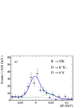
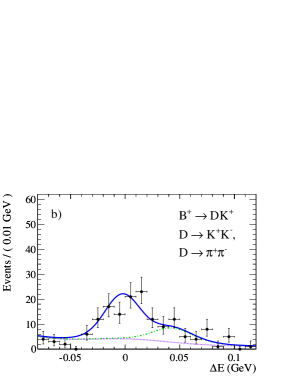
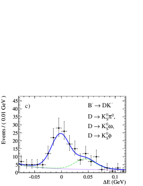
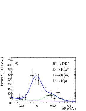
Figure 2: $\Delta E$ projections of the fits to the data, split into subsets of definite $C\!P$ of the $D$ candidate and charge of the $B$ candidate: a) $B^{-}{\rightarrow}D_{C\!P+}K^{-}$, b) $B^{+}{\rightarrow}D_{C\!P+}K^{+}$, c) $B^{-}{\rightarrow}D_{C\!P-}K^{-}$, d) $B^{+}{\rightarrow}D_{C\!P-}K^{+}$. The curves are the full PDF (solid, blue), and $B{\rightarrow}D\pi$ (dash-dotted, green) stacked on the remaining backgrounds (dotted, purple). The region between the solid and the dash-dotted lines represents the $B{\rightarrow}DK$ contribution. We show the subsets of the data sample in which the track $h$ from the $B$ decay is identified as a kaon. We require candidates to lie inside the signal-enriched region defined in Sec. IV, except for the plotted variable.

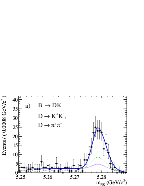
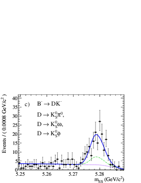
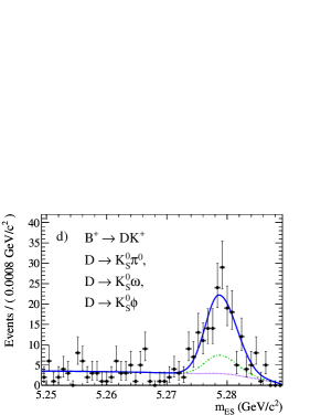
Figure 3: $m_{\rm ES}$ projections of the fits to the data, split into subsets of definite $C\!P$ of the $D$ candidate and charge of the $B$ candidate: a) $B^{-}\rightarrow D_{C\!P+}K^{-}$, b) $B^{+}\rightarrow D_{C\!P+}K^{+}$, c) $B^{-}\rightarrow D_{C\!P-}K^{-}$, d) $B^{+}\rightarrow D_{C\!P-}K^{+}$. We show the subsets of the data sample in which the track $h$ from the $B$ decay is identified as a kaon. See caption of Fig. 2 for line definitions. Only a subrange of the whole fit range is shown in order to provide a closer view of the signal peak.

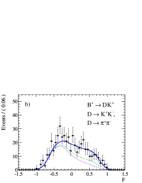
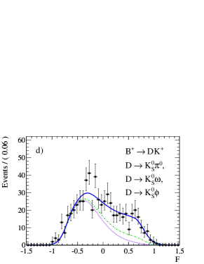
Figure 4: $\mathcal{F}$ projections of the fits to the data, split into subsets of definite $C\!P$ of the $D$ candidate and charge of the $B$ candidate: a) $B^{-}\rightarrow D_{C\!P+}K^{-}$, b) $B^{+}\rightarrow D_{C\!P+}K^{+}$, c) $B^{-}\rightarrow D_{C\!P-}K^{-}$, d) $B^{+}\rightarrow D_{C\!P-}K^{+}$. We show the subsets of the data sample in which the track $h$ from the $B$ decay is identified as a kaon. See caption of Fig. 2 for line definitions.

Figure 5: Projections of (a) $\Delta E$, (b) $m_{\rm ES}$, and (c) $\mathcal{F}$ variables of the fit to the $B^{\pm}\rightarrow Dh^{\pm}$, $D^{0}\rightarrow K^{-}\pi^{+}$ flavor mode. No requirements are put on the PID of the track $h$ from the $B$ decay and on the fit variables not plotted. See caption of Fig. 2 for line definitions.

The statistical significance of a non-zero $A_{C\!P\!+}$ value is determined from the maximum value of the likelihood function of the nominal fit and that of a dedicated null-hypothesis fit, where $A_{C\!P\!+}$ was fixed to zero,

$$S_{\rm stat}=\sqrt{2\ln(\mathcal{L}_{\rm nom}/\mathcal{L}_{\rm null})}=3.7.$$ (45)

Taking into account systematic uncertainties, the statistical significance of $A_{C\!P+}$ is slightly decreased to:

$$S_{{\rm stat}+{\rm syst}}=\frac{S_{\rm stat}}{\sqrt{1+\frac{\sigma_{\rm syst}^{2}}{\sigma_{\rm stat}^{2}}}}=3.6.$$ (46)

This constitutes evidence for direct $C\!P$ violation in charged $B$ decays and the first evidence of direct $C\!P$ violation in $B\rightarrow DK$.

We constrain the CKM angle $\gamma$, the strong phase $\delta_{B}$, and the amplitude ratio $r_{B}$ from the present measurement by adopting the frequentist procedure also exploited in babar_dk_DALITZ_PRD . We define a multivariate Gaussian likelihood function

$$\mathcal{L}(\gamma,\delta_{B},r_{B})=\frac{1}{N}\exp\left(-\frac{1}{2}(\vec{y}-\vec{y_{\rm t}})^{T}V_{\rm cov}^{-1}(\vec{y}-\vec{y_{\rm t}})\right)$$ (47)

relating the experimentally measured observables $\vec{y}$ and their statistical and systematic covariance matrices $V_{\rm cov}=V_{\rm stat}+V_{\rm syst}$ with the corresponding truth parameters $\vec{y_{\rm t}}=\vec{y_{\rm t}}(\gamma,\delta_{B},r_{B})$ calculated using Eqns. 3 and 4. The matrices $V_{\rm stat}$ and $V_{\rm syst}$ are constructed from Eqns. 35-44. The normalization is $N=(2\pi)^{2}\sqrt{|V_{\rm cov}|}$. We then define a $\chi^{2}$-function as

$$\chi^{2}(\gamma,\delta_{B},r_{B})=-2\ln\mathcal{L}(\gamma,\delta_{B},r_{B}).$$ (48)

Due to the inherent eight-fold ambiguity of the GLW method there are eight equivalent minima of the $\chi^{2}$-function, $\chi^{2}_{\min}$, which correspond to the same value of $r_{B}$ and to eight alternative solutions for $(\gamma,\delta_{B})$. To evaluate the confidence level of a certain truth parameter (for example $\gamma$) at a certain value ($\gamma_{0}$) we consider the value of the $\chi^{2}$-function at the new minimum, $\chi^{2}_{\min}(\gamma_{0},\delta_{B}^{\prime},r_{B}^{\prime})$, satisfying $\Delta\chi^{2}=\chi^{2}_{\min}(\gamma_{0},\delta_{B}^{\prime},r_{B}^{\prime})-\chi^{2}_{\min}\geq 0$. In a purely Gaussian situation for the truth parameters the CL is given by the probability that $\Delta\chi^{2}$ is exceeded for a $\chi^{2}$-distribution with one degree of freedom:

$${1-\rm CL}=\frac{1}{\sqrt{2}\,\Gamma(1/2)}\int_{\Delta\chi^{2}}^{\infty}e^{-t/2}t^{-1/2}\,{\rm d}t.$$ (49)

A more accurate approach is to take into account the non-linearity of the GLW relations, Eqns. 3 and 4. In this case one should consider $\Delta\chi^{2}$ as a test statistic, and calculate $(1-\rm CL)$ by means of a Monte Carlo procedure, described in the following. For a certain value of interest $(\gamma_{0})$, we:

1. calculate $\Delta\chi^{2}=\chi^{2}_{\min}(\gamma_{0},\delta_{B}^{\prime},r_{B}^{\prime})-\chi^{2}_{\min}$ as before;

2. generate a “toy” result $A_{C\!P\!\pm}^{\prime}$, $R_{C\!P\!\pm}^{\prime}$, using Eq. 47 with values $\gamma_{0}$, $\delta_{B}^{\prime}$, $r_{B}^{\prime}$ as the PDF;

3. calculate $\Delta\chi^{2\prime}$ of the toy result as in the first step, i.e. minimize again with respect to $\delta_{B}$ and $r_{B}$;

4. calculate $(1-\rm CL)$ as the fraction of toy results which perform better than the measured data, i.e. $1-\rm CL=N(\Delta\chi^{2}>\Delta\chi^{2\prime})/N_{\rm toy}$.

Figures 6 and 7 illustrate 1-CL as a function of $\gamma$ and $r_{B}$ as obtained from this study. From these distributions we extract 68% and 95% CL confidence intervals for $\gamma$ and $r_{B}$, as summarized in Table 7. Due to the $\gamma\leftrightarrow\delta_{B}$ ambiguity of the GLW method, the 1D CL intervals for $\delta_{B}$ are identical to those for $\gamma$. At the 68% CL we are able to distinguish six out of eight solutions for $\gamma$ (and $\delta_{B}$), two of which are in good agreement with the current world averages PDG2008 . At the 95% CL we are able to exclude the intervals $[0^{\circ},7.0^{\circ}]$, $[173.0^{\circ},187.0^{\circ}]$ and $[353.0^{\circ},360^{\circ}]$ for $\gamma$ and $\delta_{B}$. For $r_{B}$ we deduce at 68% CL:

$$r_{B}=0.35^{+0.10}_{-0.11}\mathrm{(stat+syst)}.$$ (50)

Table 7: 68% and 95% CL intervals for the parameters $\gamma$, and $r_{B}$, taking into account both statistical and systematic uncertainties. The confidence intervals for $\delta_{B}$ are identical to those for $\gamma$ due to the intrinsic $\gamma\leftrightarrow\delta_{B}$ ambiguity of the GLW method.

	$\gamma\mod 180\,[{}^{\circ}]$	$r_{B}$
68% CL	$[11.3,22.7]$	$[0.24,0.45]$
	$[80.8,99.2]$
	$[157.3,168.7]$
95% CL	$[7.0,173.0]$	$[0.06,0.51]$

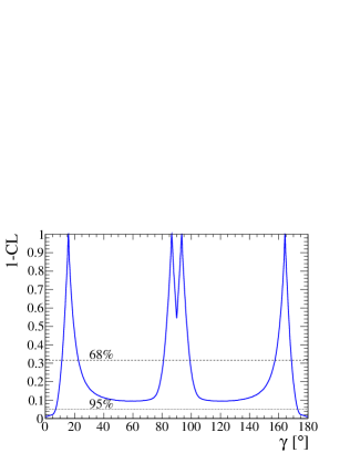
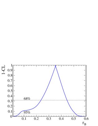
Figure 6: 1-CL as a function of $\gamma$ (top) and $r_{B}$ (bottom). Both statistical and systematic uncertainties are taken into account. For the angle $\gamma$, the plot is identical in the range $[180^{\circ},360^{\circ}]$. The horizontal lines show the 68% CL (dashed) and the 95% CL (dotted). Due to the symmetry of Eqns. 3 and 4 the plot for the strong phase $\delta_{B}$ is identical to the one for $\gamma$.

Figure 7: Contours at 68% (dotted, red) and 95% (solid, green) 2-dimensional CL in the $(\gamma,r_{B})$ and $(\gamma,\delta_{B})$ planes. See also the caption of Fig. 6 regarding symmetries.

In order to facilitate the future combination of these measurements with the results of the Dalitz plot analysis of $B^{\pm}\rightarrow DK^{\pm}$, $D\rightarrow K^{0}_{\scriptscriptstyle S}h^{+}h^{-}$ decays ($h=\pi,K$) babar_dk_DALITZ_PRL , we recompute the GLW parameters after excluding from the nominal fit the $D_{C\!P-}\rightarrow K^{0}_{\scriptscriptstyle S}\phi$ ($\phi\rightarrow K^{+}\kern-1.60004ptK^{-}$) subsample. The sample obtained in this way is statistically independent of that selected in babar_dk_DALITZ_PRL . The final values of the GLW parameters that we measure in this case are:

$$A_{C\!P\!+} = \phantom{-}0.25\pm 0.06\mathrm{(stat)}\pm 0.02\mathrm{(syst)}\,,$$ (51)

$$A_{C\!P\!-} = -0.08\pm 0.07\mathrm{(stat)}\pm 0.02\mathrm{(syst)}\,,$$ (52)

$$R_{C\!P\!+} = \phantom{-}1.18\pm 0.09\mathrm{(stat)}\pm 0.05\mathrm{(syst)}\,,$$ (53)

$$R_{C\!P\!-} = \phantom{-}1.03\pm 0.09\mathrm{(stat)}\pm 0.04\mathrm{(syst)}\,.$$ (54)

The statistical correlations among these four quantities are:

$$C_{\mathrm{(stat)}}[\vec{y}]=\left(\begin{array}[]{cccc}1&0&-0.08&0\\ &1&0&0.04\\ &&1&0.09\\ &&&1\end{array}\right)\ ,$$ (59)

and the systematic correlations are

$$C_{\mathrm{(syst)}}[\vec{y}]=\left(\begin{array}[]{cccc}1&0.56&-0.06&0\\ &1&0&0\\ &&1&0.12\\ &&&1\end{array}\right).$$ (64)

To compare the results obtained after removing the $D_{C\!P-}\rightarrow K^{0}_{\scriptscriptstyle S}\phi$ subsample with those from the $B^{\pm}\rightarrow DK^{\pm},D\rightarrow K^{0}_{\scriptscriptstyle S}h^{+}h^{-}$ analyses, which are expressed in terms of the variables $x_{\pm}=r_{B}\cos(\delta_{B}\pm\gamma)$ and $y_{\pm}=r_{B}\sin(\delta_{B}\pm\gamma)$, we use the GLW parameters measured in this way to determine the quantities $x_{\pm}$ through the relations:

$$x_{\pm}=\frac{1}{4}\left[R_{C\!P\!+}(1\mp A_{C\!P\!+})-R_{C\!P\!-}(1\mp A_{C\!P\!-})\right]\,.$$ (65)

We obtain

$$x_{+} = -0.057\pm 0.039\mathrm{(stat)}\pm 0.015\mathrm{(syst)}\,,$$ (66)

$$x_{-} = \phantom{-}0.132\pm 0.042\mathrm{(stat)}\pm 0.018\mathrm{(syst)}\,.$$ (67)

These results are in good agreement with the current world averages HFAG and have precision close to the single most precise measurements babar_dk_DALITZ_PRL . We also measure $r_{B}^{2}$, which provides a constraint on $x_{\pm}$ and $y_{\pm}$ via $r_{B}^{2}=x_{\pm}^{2}+y_{\pm}^{2}$, from

$$r_{B}^{2}=\frac{1}{2}(R_{C\!P\!+}+R_{C\!P\!-}-2)\,.$$ (68)

We determine:

$$r_{B}^{2}=0.105\pm 0.067\mathrm{(stat)}\pm 0.035\mathrm{(syst)}\,.$$ (69)

The constraints that could be placed on the quantities $y_{\pm}$ from these measurements, by exploiting the relation $r_{B}^{2}=x_{\pm}^{2}\pm y_{\pm}^{2}$, are much weaker than those provided by the $B^{\pm}\rightarrow DK^{\pm}$, $D\rightarrow K^{0}_{\scriptscriptstyle S}h^{+}h^{-}$ analysis.

As a final check of consistency we consider the quantity $a$,

$$a=A_{C\!P\!+}R_{C\!P\!+}+A_{C\!P\!-}R_{C\!P\!-}\,.$$ (70)

From Eqns. 3 and 4 one expects $a$ to satisfy $a=0$. We measure $a=0.19\pm 0.11\mathrm{(stat+syst)}$, which is compatible with 0.

IX Summary

Using the entire dataset collected by BABAR at the $e^{+}e^{-}$ center-of-mass energy close to the $\mathchar 28935\relax{(4S)}$ mass, we have reconstructed $B^{\pm}\rightarrow DK^{\pm}$ decays, with $D$ mesons decaying to non-$C\!P$ ($K\pi$), $C\!P$-even ($K^{+}\kern-1.60004ptK^{-}$, $\pi^{+}\pi^{-}$) and $C\!P$-odd ($K^{0}_{\scriptscriptstyle S}\pi^{0}$, $K^{0}_{\scriptscriptstyle S}\phi$, $K^{0}_{\scriptscriptstyle S}\omega$) eigenstates.

Through an improved analysis method compared to the previous BABAR measurement babar_d0k_GLW_PRD and through an enlarged dataset, corresponding to an increase in integrated luminosity at the $\mathchar 28935\relax{(4S)}$ peak from 348$\mbox{\,fb}^{-1}$ to 426$\mbox{\,fb}^{-1}$, we obtain the most precise measurements of the GLW parameters $A_{C\!P\!\pm}$ and $R_{C\!P\!\pm}$ to date:

$$A_{C\!P\!+} = \phantom{-}0.25\pm 0.06\mathrm{(stat)}\pm 0.02\mathrm{(syst)}\,,$$

$$A_{C\!P\!-} = -0.09\pm 0.07\mathrm{(stat)}\pm 0.02\mathrm{(syst)}\,,$$

$$R_{C\!P\!+} = \phantom{-}1.18\pm 0.09\mathrm{(stat)}\pm 0.05\mathrm{(syst)}\,,$$

$$R_{C\!P\!-} = \phantom{-}1.07\pm 0.08\mathrm{(stat)}\pm 0.04\mathrm{(syst)}\,.$$

We measure a value of $A_{C\!P\!+}$ which is 3.6 standard deviations from zero, which constitutes the first evidence for direct $C\!P$ violation in $B\rightarrow DK$ decays.

From the measured values of the GLW parameters, we extract confidence intervals for the CKM angle $\gamma$, the strong phase $\delta_{B}$, and the amplitude ratio $r_{B}$, using a frequentist approach, taking into account both statistical and systematic uncertainties. At the 68% CL we find that both $\gamma$ and $\delta_{B}$ (modulo $180^{\circ}$) belong to one of the three intervals $[11.3^{\circ},22.7^{\circ}]$, $[80.8^{\circ},99.2^{\circ}]$ or $[157.3^{\circ},168.7^{\circ}]$, and that

$$r_{B}\in[0.24,0.45].$$

At 95% CL, we exclude the intervals $[0^{\circ},7.0^{\circ}]$, $[173.0^{\circ},187.0^{\circ}]$ and $[353.0^{\circ},360^{\circ}]$ for $\gamma$ and $\delta_{B}$, and measure

$$r_{B}\in[0.06,0.51].$$

Our results are in agreement with the current world averages PDG2008 .

To facilitate the combination of these measurements with the results of our Dalitz plot analysis of $B^{\pm}\rightarrow DK^{\pm}$, $D\rightarrow K^{0}_{\scriptscriptstyle S}h^{+}h^{-}$ $(h=K,\ \pi)$ babar_dk_DALITZ_PRL , we exclude the $D\rightarrow K^{0}_{\scriptscriptstyle S}\phi$, $\phi\rightarrow K^{+}\kern-1.60004ptK^{-}$ channel from this analysis – thus removing events selected also in babar_dk_DALITZ_PRL – and then determine

$$A_{C\!P\!-} = -0.08\pm 0.07\mathrm{(stat)}\pm 0.02\mathrm{(syst)}\,,$$

$$R_{C\!P\!-} = \phantom{-}1.03\pm 0.09\mathrm{(stat)}\pm 0.04\mathrm{(syst)}\,.$$

For comparison with the results of the $B^{\pm}\rightarrow DK^{\pm}$, $D\rightarrow K^{0}_{\scriptscriptstyle S}h^{+}h^{-}$ analyses, which are expressed in terms of the variables $x_{\pm}=r_{B}\cos(\delta_{B}\pm\gamma)$ and $y_{\pm}=r_{B}\sin(\delta_{B}\pm\gamma)$, we express our results for the GLW observables in terms of $x_{+}$ and $x_{-}$. We measure

$$x_{+} = -0.057\pm 0.039\mathrm{(stat)}\pm 0.015\mathrm{(syst)}\,,$$

$$x_{-} = \phantom{-}0.132\pm 0.042\mathrm{(stat)}\pm 0.018\mathrm{(syst)}\,,$$

at 68% CL. These results are in good agreement with the current world averages HFAG and have precision comparable to the single most precise measurements babar_dk_DALITZ_PRL . We also evaluate $r_{B}$ after the exclusion of the $D\rightarrow K^{0}_{\scriptscriptstyle S}\phi$ channel, and obtain a weak constraint on $r_{B}^{2}=x_{\pm}^{2}\pm y_{\pm}^{2}$:

$$r_{B}^{2}=0.105\pm 0.067\mathrm{(stat)}\pm 0.035\mathrm{(syst)}$$

at 68% CL.

X Acknowledgements

We are grateful for the extraordinary contributions of our PEP-II colleagues in achieving the excellent luminosity and machine conditions that have made this work possible. The success of this project also relies critically on the expertise and dedication of the computing organizations that support BABAR. The collaborating institutions wish to thank SLAC for its support and the kind hospitality extended to them. This work is supported by the US Department of Energy and National Science Foundation, the Natural Sciences and Engineering Research Council (Canada), the Commissariat à l’Energie Atomique and Institut National de Physique Nucléaire et de Physique des Particules (France), the Bundesministerium für Bildung und Forschung and Deutsche Forschungsgemeinschaft (Germany), the Istituto Nazionale di Fisica Nucleare (Italy), the Foundation for Fundamental Research on Matter (The Netherlands), the Research Council of Norway, the Ministry of Education and Science of the Russian Federation, Ministerio de Ciencia e Innovación (Spain), and the Science and Technology Facilities Council (United Kingdom). Individuals have received support from the Marie-Curie IEF program (European Union), the A. P. Sloan Foundation (USA) and the Binational Science Foundation (USA-Israel).

Table 8: Fit result of the three final fits to data, before correcting for fit biases (see Section VII).

Parameter	$KK$	$\pi\pi$	$K^{0}_{\scriptscriptstyle S}\pi^{0}$	$K^{0}_{\scriptscriptstyle S}\omega$	$K^{0}_{\scriptscriptstyle S}\phi$	$K\pi$
$A_{C\!P}^{{\rm sig}(K)}$	$0.242\pm 0.065$		$-0.089\pm 0.066$			$-0.008\pm 0.022$
$A_{C\!P}^{{\rm sig}(\pi)}$	$0.003\pm 0.015$		$-0.009\pm 0.014$			$-0.0116\pm 0.0050$
$R_{K/\pi}$	$0.0897\pm 0.0063$		$0.0808\pm 0.0056$			$0.0753\pm 0.0018$
$m$	$0.0204\pm 0.0030$		$0.0206\pm 0.0029$			$0.02143\pm 0.00089$
$A_{C\!P,f}^{B\kern 1.25995pt\overline{\kern-1.25995ptB}{}}$	$-0.004\pm 0.045$	$-0.043\pm 0.047$	n/a	n/a	n/a	$-0.043\pm 0.017$
$A_{C\!P,p}^{q\overline{q}}$	$0.012\pm 0.016$	$-0.016\pm 0.018$	$-0.002\pm 0.011$	$0.012\pm 0.020$	$-0.069\pm 0.060$	$-0.027\pm 0.016$
$A_{C\!P,f}^{q\overline{q}}$	$-0.004\pm 0.011$	$-0.0044\pm 0.0098$	$0.0021\pm 0.0071$	$-0.004\pm 0.013$	$0.001\pm 0.039$	$-0.0016\pm 0.0068$
$f^{q\overline{q}}_{\mathcal{F}}$	$0.326\pm 0.026$	$0.49$ (fixed)	$0.520\pm 0.030$	$0.27$ (fixed)	n/a	$0.396\pm 0.018$
$\sigma^{q\overline{q}}_{\mathcal{F},l,1}$	$0.160\pm 0.016$	$0.258\pm 0.023$	$0.206\pm 0.014$	$0.175\pm 0.034$	$0.2758\pm 0.0092$	$0.198\pm 0.014$
$\sigma^{q\overline{q}}_{\mathcal{F},l,2}$	$0.1742\pm 0.0020$	$0.2047\pm 0.0024$	$0.1546\pm 0.0015$	$0.1963\pm 0.0028$	n/a	$0.1965\pm 0.0017$
$\sigma^{q\overline{q}}_{\mathcal{F},r,1}$	$0.312\pm 0.011$	$0.329\pm 0.011$	$0.3541\pm 0.0068$	$0.317\pm 0.019$	$0.447\pm 0.014$	$0.3068\pm 0.0061$
$\sigma^{q\overline{q}}_{\mathcal{F},r,2}$	$0.231\pm 0.014$	$0.268\pm 0.018$	$0.275\pm 0.020$	$0.238\pm 0.013$	n/a	$0.237\pm 0.010$
$\sigma_{\mbox{$\Delta E$},\mbox{$m_{\rm ES}$}}^{B\kern 1.25995pt\overline{\kern-1.25995ptB}{}}$	n/a	n/a	n/a	n/a	n/a	$0.01048\pm 0.00057$
$a_{\mbox{$\Delta E$}}^{q\overline{q}}$	$-0.96\pm 0.14$	$-0.71\pm 0.14$	$-0.924\pm 0.099$	$-1.04\pm 0.18$	$-0.48$ (fixed)	$-0.88\pm 0.10$
$\mu_{\mbox{$\Delta E$}}$	$-2.62\pm 0.32$	$-1.36\pm 0.57$	$-1.80\pm 0.35$	$-2.87\pm 0.59$	$-0.95\pm 0.75$	$-1.527\pm 0.092$
$\sigma_{\mbox{$\Delta E$}}$	$16.63\pm 0.27$	$14.82\pm 0.49$	$17.01\pm 0.29$	$16.10\pm 0.52$	$15.82\pm 0.60$	$15.424\pm 0.076$
$\mu_{\mbox{$m_{\rm ES}$}}$	$5278.56\pm 0.12$	$5278.61\pm 0.20$	$5278.62\pm 0.12$	$5278.50\pm 0.22$	$5278.99\pm 0.25$	$5278.586\pm 0.033$
$\sigma_{\mbox{$m_{\rm ES}$},l}$	$2.207\pm 0.081$	$2.12\pm 0.15$	$2.299\pm 0.084$	$2.11\pm 0.16$	$2.33\pm 0.17$	$2.210\pm 0.022$
$\sigma_{\mbox{$m_{\rm ES}$},r}$	$2.897\pm 0.081$	$2.83\pm 0.15$	$2.922\pm 0.084$	$3.08\pm 0.16$	$2.72\pm 0.17$	$2.852\pm 0.023$
$N_{p}^{B\kern 1.25995pt\overline{\kern-1.25995ptB}{}}$	$79\pm 29$	$346\pm 52$	$176\pm 43$	$180\pm 48$	$3$ (fixed)	$328\pm 40$
$N_{f}^{B\kern 1.25995pt\overline{\kern-1.25995ptB}{}}$	$1430\pm 82$	$1517\pm 142$	$1930\pm 102$	$1195\pm 109$	$119\pm 20$	$7717\pm 170$
$N_{p}^{q\overline{q}}$	$4005\pm 69$	$3456\pm 76$	$8587\pm 101$	$2675\pm 68$	$284\pm 17$	$4722\pm 77$
$N_{f}^{q\overline{q}}$	$10890\pm 125$	$13019\pm 176$	$21657\pm 172$	$6673\pm 124$	$716\pm 29$	$28007\pm 205$
$N^{{\rm sig}(\pi)}_{\rm tot}$	$4091\pm 70$	$1230\pm 41$	$4182\pm 73$	$1440\pm 45$	$648\pm 27$	$44631\pm 232$

References

• (1) N. Cabibbo, Phys. Rev. Lett. 10, 531 (1963).
• (2) M. Kobayashi and T. Maskawa, Prog. Theor. Phys. 49, 652 (1973).
• (3) J. Charles et al., Eur. Phys. J. C 41, 1 (2005), and updates at http://ckmfitter.in2p3.fr.
• (4) M. Gronau and D. Wyler, Phys. Lett. B265, 172 (1991).
• (5) M. Gronau and D. London, Phys. Lett. B253, 483 (1991).
• (6) D. Atwood, I. Dunietz, and A. Soni, Phys. Rev. Lett. 78, 3257 (1997).
• (7) D. Atwood, I. Dunietz, and A. Soni, Phys. Rev. D 63, 036005 (2001).
• (8) A. Giri, Y. Grossman, A. Soffer, and J. Zupan, Phys. Rev. D 68, 054018 (2003).
• (9) BABAR Collaboration, B. Aubert et al., Phys. Rev. D 77, 111102 (2008).
• (10) BABAR Collaboration, B. Aubert et al., Phys. Rev. D 78, 092002 (2008).
• (11) BABAR Collaboration, B. Aubert et al., Phys. Rev. D 80, 092001 (2009).
• (12) BABAR Collaboration, B. Aubert et al., Phys. Rev. D 72, 032004 (2005).
• (13) BABAR Collaboration, B. Aubert et al., Phys. Rev. D 76, 111101(R) (2007).
• (14) BABAR Collaboration, B. Aubert et al., Phys. Rev. D 80, 031102(R) (2009).
• (15) BABAR Collaboration, B. Aubert et al., Phys. Rev. D 78, 034023 (2008).
• (16) BABAR Collaboration, B. Aubert et al., arXiv:1005.1096, (2010), submitted to Phys. Rev. Lett.
• (17) BABAR Collaboration, B. Aubert et al., Phys. Rev. D 79, 072003 (2009).
• (18) Y. Grossman, A. Soffer, and J. Zupan, Phys. Rev. D 72, 031501 (2005).
• (19) Belle Collaboration, K. Abe et al., Phys. Rev. D 73, 051106 (2006).
• (20) CDF Collaboration, T. Aaltonen et al., Phys. Rev. D 81, 031105(R) (2010).
• (21) HFAG, E. Barberio et al., arXiv:0808.1297, and updates at http://www.slac.stanford.edu/xorg/hfag.
• (22) BABAR Collaboration, B. Aubert et al., Nucl. Instrum. Methods Phys. Res., Sect. A 479, 1 (2002).
• (23) GEANT4 Collaboration, S. Agostinelli et al., Nucl. Instrum. Methods Phys. Res., Sect. A 506, 250 (2003).
• (24) D. J. Lange, Nucl. Instrum. Methods Phys. Res., Sect. A 462, 152 (2001).
• (25) Particle Data Group, C. Amsler et al., Phys. Lett. B667, 1 (2008), and updates at http://pdg.lbl.gov.
• (26) G. C. Fox and S. Wolfram, Phys. Rev. Lett. 41, 1581 (1978).
• (27) M. J. Oreglia, Ph.D. thesis, SLAC-R-236 (1980), Appendix D.
• (28) ARGUS Collaboration, H. Albrecht et al., Phys. Lett. B 241, 278 (1990).
• (29) G. Marchiori, Ph.D. thesis, SLAC-R-947 (2005).