Impact of random obstacles on the dynamics of a dense colloidal fluid

Abstract

Using molecular dynamics simulations we study the slow dynamics of a colloidal fluid annealed within a matrix of obstacles quenched from an equilibrated colloidal fluid. We choose all particles to be of the same size and to interact as hard spheres, thus retaining all features of the porous confinement while limiting the control parameters to the packing fraction of the matrix, $\phi_{\mathrm{m}}$, and that of the fluid, $\phi_{\mathrm{f}}$. We conduct detailed investigations on several dynamic properties, including the tagged-particle and collective intermediate scattering functions, the mean-squared displacement, and the van Hove function. We show the confining obstacles to profoundly impact the relaxation pattern of various quantifiers pertinent to the fluid. Varying the type of quantifier (tagged-particle or collective) as well as $\phi_{\mathrm{m}}$ and $\phi_{\mathrm{f}}$, we unveil both discontinuous and continuous arrest scenarios. Furthermore, we discover subdiffusive behavior and demonstrate its close connection to the matrix structure. Our findings partly confirm the various predictions of a recent extension of mode-coupling theory to the quenched-annealed protocol.

I Introduction

Fluids that are brought into contact with a disordered porous matrix drastically change their physical properties. Over the past two or three decades numerous experimental and theoretical investigations have been dedicated to studying this phenomenon Gelb et al. (1999); Rosinberg (1999); McKenna (2000, 2003); Alcoutlabi and McKenna (2005); McKenna (2007). The remarkable efforts that have been undertaken to obtain a deeper understanding of the underlying mechanisms are not only motivated by academic interest. Fluids confined in disordered porous environments play a key role in a wide spectrum of applied problems ranging from technological applications over chemical engineering to biophysical systems. Thus, a deeper understanding of why fluids change their properties under such external conditions is of great practical relevance.

From a theoretical viewpoint, a quantitative description of such systems is a formidable challenge for several reasons. For one, it is difficult to reliably and realistically represent the matrices found in experiments or technological applications (such as aerogels or vycor). Having chosen some model for the confinement, an even more demanding task is to formulate a theoretical framework that is able to appropriately describe the interplay of connectivity and confinement of the pores pertinent to the matrix. Even after reducing such system to the so-called quenched-annealed (QA) model, where for simplicity the matrix is assumed to be an instantaneously-frozen configuration of an equilibrated fluid, an appropriate theory is highly intricate. Madden and Glandt Madden and Glandt (1988); Madden (1992), and later Given and Stell Given (1992); Given and Stell (1992, 1994), derived a formalism based on statistical mechanics that considers the system to be a peculiar mixture with the matrix being one of the components. Within their framework, Given and Stell derived Ornstein-Zernike-type integral equations (the so-called replica Ornstein-Zernike equations, ROZ) that—in combination with a suitable closure relation—allow to determine the static correlators and the thermodynamic properties of a QA system Rosinberg et al. (1994); Kierlik et al. (1995, 1997); Paschinger and Kahl (2000); Schöll-Paschinger et al. (2001). Their formalism is based on a twofold thermodynamic averaging procedure: one over all possible fluid configurations for a fixed matrix realization, the other one over all possible matrix configurations. This double-averaging procedure is adapted to the letter in computer simulation studies of fluids confined in disordered porous materials; in terms of computing time this is a demanding enterprise.

Until few years ago most theoretical and simulation studies focused on the static properties of QA systems such as structure and phase behavior. In contrast, comparatively little effort had been devoted to the dynamic properties. The main obstacles inhibiting such investigations were, on one side, the lack of a suitable theoretical framework that would have allowed to reliably evaluate the dynamic correlation functions of the fluid particles, and, on the other hand, limitations in computational power for simulations when explicitly performing the above-mentioned double-averaging procedure. To the best of our knowledge, the first simulation studies dedicated to the dynamic properties of fluids in disordered porous confinement were performed by Gallo and Rovere Gallo et al. (2002, 2003a, 2003b), followed shortly after by Kim Kim (2003). In this context it is worth mentioning similar investigations on the Lorentz gas model Höfling et al. (2006) and on binary mixtures in which particles are characterized by a large disparity in size Voigtmann and Horbach (2009); Moreno and Colmenero (2006) or mass Fenz et al. (2009), i.e., systems that can be viewed to be closely related to QA systems.

Over the past years, major breakthroughs have been achieved in describing theoretically the dynamic properties of fluids in confined in porous media. In particular, use was made of mode-coupling theory (MCT) Krakoviack (2005, 2007, 2009) and of the self-consistent generalized Langevin equation (SCGLE) theory Chávez-Rojo et al. (2008), both of which rely on inferring the dynamics of a system from its static structure. MCT has played over the last decades a central role in describing the dynamic properties of fluids Götze (1999), including in particular the glass transition. Krakoviack succeeded in deriving MCT-type equations for the dynamic correlation functions, which require as an input the static correlation functions of the annealed fluid, which in turn are obtained from the ROZ equations. Subsequently, Krakoviack solved these equations for the specific case of a hard-sphere fluid confined in a disordered matrix of hard-sphere particles of equal size and evaluated single-particle and collective correlation functions of the system. Based on this knowledge, a kinetic diagram was traced out in the parameter space spanned by the packing fraction of the fluid and that of the matrix, indicating the regions in which the system is in an arrested or in a nonarrested state. The resulting kinetic diagram is very rich and quite surprising: the regions of arrested and nonarrested states are separated by a line along which at small matrix packing fractions type-B transitions and at intermediate matrix packing fractions type-A transitions occur. As a peculiar feature of this line, a re-entrant glass transition is predicted for intermediate matrix and small fluid packing fractions. Additionally, in the region of nonarrested states a continuous diffusion-localization transition is observed. However, we emphasize that the combined ROZ+MCT framework predicts ideal transitions, whereas in experiment or simulation transitions will always be smeared out.

Throughout this contribution we employ the type-A/type-B terminology that is conventionally used to characterize the behavior of a dynamic correlator as an ideal transition occurs. This terminology refers to the decay pattern of the correlator as well as to the behavior of its long-time limit upon crossing a dynamic transition. In a “type-A” transition a correlator relaxes in a single step, and its long-time limit may assume arbitrarily small nonzero values. In a transition of “type-B,” on the other hand, a correlator decays in a distinct two-step pattern; upon crossing the transition the second decay step is delayed to infinity and the long-time limit of the correlator jumps from zero to a nonzero value. The type-B behavior is well-known from bulk glass formers Götze and Sjögren (1992) and is usually attributed to a “cage effect” imposed upon fluid particles by their neighbors.

This remarkably rich phase behavior has motivated simulation studies which—as a consequence of the considerable increase in available computation power—have meanwhile come within reach. Short accounts have been given in Kurzidim et al. (2009) and Kim et al. (2009). In this contribution we elaborate on our investigations on the dynamic behavior of a fluid confined in a disordered porous matrix within the QA picture. For simplicity, and for congruence with the theoretical studies Krakoviack (2005, 2007, 2009), we consider a fluid of hard spheres confined in a disordered matrix formed by hard spheres of the same size. Investigations are based on event-driven molecular dynamics simulations. Within the two-dimensional parameter space we focus mainly on three representative pathways to put the theoretical predictions to a thorough test: (i) a path at constant low matrix packing fraction, probing the existence of the continuous type-B transition, (ii) a path at constant intermediate matrix packing fraction, probing the discontinuous type-A transition and the re-entrant scenario, and (iii) a path at intermediate, constant fluid packing fraction, probing the diffusion-localization transition. Results are summarized in kinetic diagrams, where we consider—complementing our previous communication—different criteria to define dynamical arrest. We compare our simulation results with the predictions of MCT, which, however, is not straightforward due to the ideal nature of the latter.

The paper is organized as follows: in Sec. II we present the model and our simulation method, transferring the rather lengthy description of the system setup to Appendix A. Results are compiled in Sec. III: we start with the static structure of the system and then discuss various methods of how to define slowing down and the ensuing kinetic diagrams. In the subsequent three subsections we discuss the intermediate scattering functions and the mean-squared displacement along the three aforementioned paths through parameter space. The final subsection of Sec. III shall deal with the van Hove correlation function in order to discuss trapping. In Sec. IV we extend the analysis of the intermediate scattering functions to discuss the arrest scenarios in more detail. The paper closes with concluding remarks alongside with an outlook on future work required to settle questions yet open. The aforementioned Appendix A is succeeded by Appendix B in which we elaborate on the issue of the effects of system size on the dynamical correlation functions.

II Model and Methods

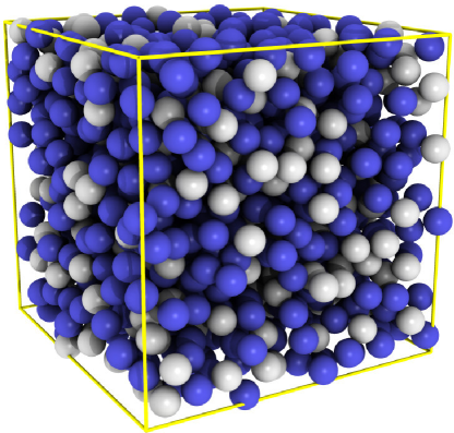
Figure 1: (Color online) Snapshot of a quenched-annealed mixture of hard spheres at $\phi_{\mathrm{m}}=0.25$ and $\phi_{\mathrm{f}}=0.10$. Dark (blue): matrix particles, light (gray): fluid particles.

For the purpose of this work we opted for the “quenched-annealed” (QA) protocol since it is well-defined, well-tractable by theory, and involves only a small number of parameters. In this protocol both the porous confinement and the confined fluid are represented by a set of particles, conventionally called “matrix” and “fluid” particles or—borrowing from the typology of metallurgy—as “quenched” and “annealed” component. In this, QA systems bear resemblance to mixtures; however, the matrix particles are pinned at particular positions and act as obstacles for the fluid particles. In this work, we exclusively consider systems containing one matrix and one fluid species; quantities pertaining to those species will be designated with the subscripts “m” and “f,” respectively.

Adopting the concept of immobile obstacle particles, there are still numerous schemes for their arrangement Zhang and van Tassel (2000); Zhao et al. (2006); Kim et al. (2009); Fenz et al. (2009); Gallo et al. (2009). The QA protocol specifies the positions of the matrix particles to be frozen from an equilibrium one-component fluid; the fluid particles merely move within this matrix and do not exert influence upon it . Notably, the fluid particles may also dwell in “traps”—finite spatial domains entirely bounded by infinite potential walls formed by the confining matrix.

Since for this work we are interested in a minimal approach to the dynamics of a fluid moving in disordered confinement, we decided to exclusively employ hard-sphere (HS) interactions among the particles. This deprives the system of any inherent energy scale, rendering the only relevant system attributes to be of geometrical nature. We further reduced the parameter space by requiring all particles involved to be of the same (monodisperse) diameter $\sigma$. This introduces $\sigma$ as the unit of length used throughout this study, and leaves the system to be governed by mere packing fractions, namely the matrix packing fraction $\phi_{\mathrm{m}}$ and the fluid packing fraction $\phi_{\mathrm{f}}$. As mentioned before, this particular choice of system was examined in Krakoviack (2005, 2007, 2009). A snapshot of a typical HS-QA system at large matrix density is shown in Fig. 1.

In this work we study QA systems utilizing molecular simulations. Since we are primarily interested in dynamical features, we applied molecular dynamics (MD) simulations to track the physical time evolution of a system. All MD computations were performed using the event-driven algorithm described in Alder and Wainwright (1959); modifications to that algorithm were essentially limited to fixing particles in space in order to adapt to the QA protocol. (Notably, this adjustment invalidates the conservation of momentum and angular momentum.) As is conventional, we employed periodic (toroidal) boundary conditions and the minimum-image convention in order to mimic an infinite system.

In addition to the usual thermodynamic averaging, $\langle\mathstrut\cdots\rangle$ , the QA protocol imposes another averaging procedure over disorder, $\overline{\mathstrut\cdots}$ , so as to restore homogeneity and isotropy. Depending on the state point $(\phi_{\mathrm{m}},\phi_{\mathrm{f}})$ and the number of particles in the system, we averaged our data over at least ten matrix configurations; for selected state points, we increased that number to as much as $40$.

A nontrivial task is to find an initial system configuration given some state point. In this work, we are interested in systems in which the $N_{\mathrm{f}}$ fluid particles comprise most of the space that is left accessible to them by the $N_{\mathrm{m}}$ immobile matrix particles—i.e., high-density systems. Generating instances of the porous confinement is effortless, since for all state points of interest, $\phi_{\mathrm{m}}$ is situated well within the fluid regime when used for a one-component system of mobile particles. The problem rests in determining permissible initial positions for the $N_{\mathrm{f}}$ fluid particles. Creating an amorphous high-density configuration of bulk monodisperse hard-sphere particles already represents an interesting task, with various elaborate algorithms having been developed to accomplish this task Bennett (1972); Jodrey and Tory (1985). However, none of these algorithms are suited for adaption to the setup of HS-QA systems. This unfortunate finding prompted us to devise a custom routine which is described in detail in Appendix A.

After successful setup of a system instance, the simulation time was set to $t=0$ and an attempt to equilibrate the system using the MD routine was made. The decision whether or not the particular system realization was considered equilibrated was based on the mean-squared displacement

$$\delta r^{2}(t)=\overline{\left\langle\left|{}\mathbf{r}^{\mathrm{t}}(t)-\mathbf{r}^{\mathrm{t}}(0)\right|^{2}\right\rangle}$$ (1)

where $\mathbf{r}^{\mathrm{t}}(t)$ is the location of a tagged (superscript “$\mathrm{t}$”) fluid particle at time $t$. Note that the above definition is the one used in Sec. III and hence involves an average over matrix configurations; of course this average has to be omitted when using $\delta r^{2}(t)$ to characterize a single system realization. Also, note that the notion of a “tagged particle” does not imply the presence of an additional tracer particle.

We defined a system realization to be in equilibrium if $\delta r^{2}(t_{*})>\delta r^{2}_{*}=100$ was fulfilled. We allowed at least $t_{*}=30\,000$ time units for the system to equilibrate; for certain state points we extended $t_{*}$ to as much as the tenfold value. The conventional unit of time $\tau=\sqrt{m\sigma^{2}/k_{\mathrm{B}}T}$ used throughout this work is based upon the mass $m$ of the fluid particles, their diameter $\sigma$ (see above), and their temperature $T$ Allen and Tildesley (1987).

Data were only compiled after equilibration was attempted, using the final configuration of the equilibration run as initial configuration of the data run. Generally, the final time for data collection, $t_{\mathrm{d}}$, was chosen to be equal to the final time of the equilibration attempt, $t_{\mathrm{e}}$; in particular in some nonequilibrated systems we also used $t_{\mathrm{d}}>t_{\mathrm{e}}$ to investigate particular features of the system. For most state points, we chose $N=N_{\mathrm{m}}{+}N_{\mathrm{f}}\simeq 1000$ to be the total particle number . In order to retain reasonable statistics even close to $\phi_{\mathrm{f}}=0$, we increased $N$ to as much as $12\,000$ for elevated $\phi_{\mathrm{m}}$, such that $N_{\mathrm{f}}\geq 50$ for all state points.

III Results

III.1 Static structure

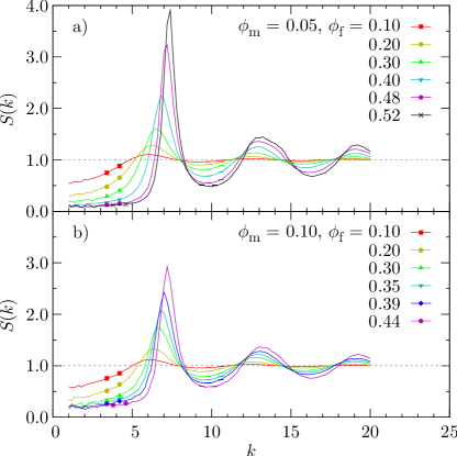
Figure 2: (Color online) Fluid-fluid static structure factor $S(k)$ for a series of $\phi_{\mathrm{f}}$ values at constant $\phi_{\mathrm{m}}$. (a) $\phi_{\mathrm{m}}=0.05$, (b) $\phi_{\mathrm{m}}=0.10$. Error bars represent one standard deviation of the mean for different system realizations.

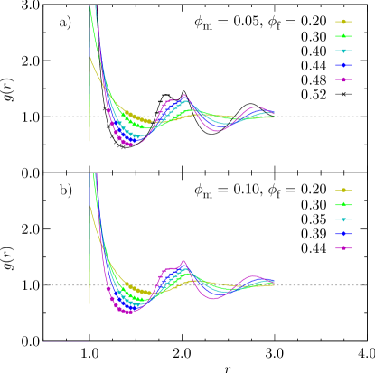
Figure 3: (Color online) Fluid-fluid radial distribution function $g(r)$ for a series of $\phi_{\mathrm{f}}$ values at constant $\phi_{\mathrm{m}}$. (a) $\phi_{\mathrm{m}}=0.05$, (b) $\phi_{\mathrm{m}}=0.10$. Error bars: see Fig. 2

The most obvious properties to inspect in our systems are simple static structural properties; this investigation was already carried out in great detail in Lomba et al. (1993). In the present context static properties are of use for a different reason: Since the particles were chosen to be of monodisperse diameter $\sigma$, crystallization might take place in the case of dilute matrices. Inspection of the radial distribution function $g(r)$ and the static structure factor $S(k)$ provides a means to determine whether or not this is the case. In fact, it is sufficient to investigate fluid-fluid correlations, $g_{\mathrm{ff}}(r)$ and $S_{\mathrm{ff}}(k)$, since only for $\phi_{\mathrm{f}}\gg\phi_{\mathrm{m}}$ systems are prone to crystallization. Therefore, the index “$\mathrm{ff}$” will henceforth be dropped.

We first consider the static structure factor

$$S(k)=\frac{4\pi}{N_{\mathrm{f}}}\leavevmode\nobreak\ \overline{\left\langle\sum_{i}^{N_{\mathrm{f}}}\sum_{j}^{N_{\mathrm{f}}}\frac{r_{ij}}{k}\sin\left({}k\,r_{ij}\right)\right\rangle}$$ (2)

where $r_{ij}=|\mathbf{r}^{\mathrm{f}}_{i}-\mathbf{r}^{\mathrm{f}}_{j}|$, and $\mathbf{r}^{\mathrm{f}}_{i}$ denotes the location of fluid particle $i$. Fig. 2 displays this function for moderate ($\phi_{\mathrm{m}}=0.1$) and for low ($\phi_{\mathrm{m}}=0.05$) matrix packing fractions, i.e., for systems particularly prone to crystallization. Clearly, all features of $S(k)$ evolve smoothly upon increasing $\phi_{\mathrm{f}}$, suggesting that no phase transition takes place. Moreover, the absence of sharp peaks for all state points indicates that no simple crystalline long-range order is present.

Related arguments hold for the radial distribution function

$$g(r)=\frac{V}{N_{\mathrm{f}}^{2}}\leavevmode\nobreak\ \overline{\left\langle\mathop{\sum\sum}_{i\neq j}^{N_{\mathrm{f}}}\delta\left({}r-r_{ij}\right)\right\rangle}$$ (3)

where $V$ is the system volume. Fig. 3 shows this function for the same matrix packing fractions as above ($\phi_{\mathrm{m}}\in\{0.1,0.05\}$). As for $S(k)$, the features of $g(r)$ develop continuously, which again supports the notion that a phase transition is absent.

Additional peaks in $g(r)$ at specific positions would be a hallmark of crystallization. For fcc- or bcc-like short-range order, the most pronounced additional peaks would be located at $r_{\mathrm{fcc}}=\Phi\sqrt{2}$ or $r_{\mathrm{bcc}}=\Phi\sqrt{3}$, where $\Phi=\{(\phi_{\mathrm{m}}+\phi_{\mathrm{f}})/\phi_{\mathrm{max}}\}^{1/3}$ and $\phi_{\mathrm{max}}=\pi/(3\sqrt{2})$ is the volume fraction of close-packed monodisperse hard spheres. For instance, for $\phi_{\mathrm{m}}=0.05$ and $\phi_{\mathrm{f}}=0.50$, crystallites would cause a peak at $r_{\mathrm{fcc}}\simeq 1.56$ or $r_{\mathrm{bcc}}\simeq 1.91$. Clearly, peaks at these positions are absent in Fig. 3. On the other hand, in both panel (a) and (b) an additional peak at $r\simeq 1.8$ emerges upon increasing $\phi_{\mathrm{f}}$. However, this peak is a well-known feature of glass-forming systems Kob and Andersen (1995) and thus provides further evidence for the absence of crystallization. We conclude that crystallites, albeit possibly temporarily present, do not play a major role in the systems under investigation.

III.2 Kinetic diagrams

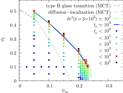
Figure 4: (Color online) Kinetic diagram based on single-particle properties (see text). Symbols: time $t_{\mathrm{s}}$ needed for $F_{\mathrm{s}}(k{=}7.0,t)$ to decay below $F_{\mathrm{s}}^{*}=0.1$. Thick solid (blue) line: interpolation through points for which $t_{\mathrm{s}}\simeq 10^{3}$. Thick dotted (green) line: arrest line based on $\delta r^{2}(t)$ from Kurzidim et al. (2009) (extended to low $\phi_{\mathrm{f}}$ values). Thin dashed and dotted (black) lines: MCT transition lines pertaining to single-particle properties from Krakoviack (2009).

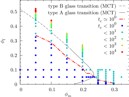
Figure 5: (Color online) Kinetic diagram based on collective properties (see text). Symbols: time $t_{\mathrm{c}}$ needed for $F_{\mathrm{c}}(k{=}7.0,t)$ to decay below $F_{\mathrm{c}}^{*}=0.1$. Thick dash-dotted (red) line: interpolation through points for which $t_{\mathrm{c}}\simeq 10^{0}$. Thin dashed and solid (black) lines: MCT transition lines pertaining to collective properties from Krakoviack (2009).

Many features of the system under investigation can be understood by means of kinetic diagrams in which the “state” of a dynamic property is indicated in the plane spanned by $\phi_{\mathrm{m}}$ and $\phi_{\mathrm{f}}$. In an earlier work Kurzidim et al. (2009) we presented a kinetic diagram based on the mean-squared displacement $\delta r^{2}(t)$. In order to classify the state of the system, we chose a mean-squared displacement $\delta r^{2}_{*}=100$ and a simulation time $t_{*}=30\,000$; if the system obeyed $\delta r^{2}(t_{*})>\delta r^{2}_{*}$ then it was considered “nonarrested,” and otherwise “arrested.” The so-constructed kinetic diagram qualitatively confirmed the behavior of the single-particle dynamics of the system at hand as predicted by MCT Kurzidim et al. (2009); Krakoviack (2009). The arrest line determined from this criterion is indicated in Fig. 4.

In Fig. 4 we present a kinetic diagram of the system under investigation based on the self-intermediate scattering function

$$F_{\mathrm{s}}(k,t)=\frac{\leavevmode\nobreak\ \leavevmode\nobreak\ \overline{\left\langle\rho_{\mathbf{k}}^{\mathrm{t}}(t)\rho_{\mathbf{-k}}^{\mathrm{t}}(0)\right\rangle}\leavevmode\nobreak\ \leavevmode\nobreak\ }{\leavevmode\nobreak\ \leavevmode\nobreak\ \overline{\left\langle\rho_{\mathbf{k}}^{\mathrm{t}}(0)\rho_{\mathbf{-k}}^{\mathrm{t}}(0)\right\rangle}\leavevmode\nobreak\ \leavevmode\nobreak\ }$$ (4)

where $\rho_{\mathbf{k}}^{\mathrm{t}}(t)=\exp\{i\mathbf{k}\cdot\mathbf{r}^{\mathrm{t}}(t)\}$ is the density of a tagged (superscript “$\mathrm{t}$”) fluid particle in $k$ space after some time $t$ has passed . The symbols in the figure indicate the times $t_{\mathrm{s}}$ needed for $F_{\mathrm{s}}(k{=}7.0,t)$ to decay below the value $F_{\mathrm{s}}^{*}=0.1$. The value $k=7.0$ was chosen to be close to the main peak in $S(k)$ in a typical high-density QA system—for instance, for $\phi_{\mathrm{m}}=0.05$ and $\phi_{\mathrm{f}}=0.50$ (cf. Fig. 2) the first peak in $S(k)$ is located at $k\simeq 7.2$; for $\phi_{\mathrm{m}}=0.25$ and $\phi_{\mathrm{f}}=0.10$ it is found at $k\simeq 6.6$.

If we let $t_{\mathrm{s}}^{*}\simeq 10^{3}$, discriminating whether for a state point $t_{\mathrm{s}}>t_{\mathrm{s}}^{*}$ (“arrested”) or $t_{\mathrm{s}}<t_{\mathrm{s}}^{*}$ (“nonarrested”) yields the thick solid (blue) line in Fig. 4. Obviously, the latter is only slightly different from the thick dotted (green) line that is obtained from the $\delta r^{2}(t)$ criterion described above. This is not unexpected since both $F_{\mathrm{s}}(k,t)$ and $\delta r^{2}(t)$ are single-particle properties, and in the Gaussian limit it is even $F_{\mathrm{s}}(k,t)=\exp\{k^{2}\delta r^{2}(t)/6\}$ Hansen and McDonald (1986). Thus, the validity of the approach chosen in Kurzidim et al. (2009) is confirmed.

In order to complement the kinetic diagrams based upon single-particle properties, in Fig. 5 we present for the first time a kinetic diagram for a collective property of the system. For comparison with the theory developed in Krakoviack (2005, 2007, 2009) we chose to operate with the connected part of the intermediate scattering function

$$F_{\mathrm{c}}(k,t)=\frac{\leavevmode\nobreak\ \leavevmode\nobreak\ \overline{\left\langle\delta\rho_{\mathbf{k}}(t)\delta\rho_{\mathbf{-k}}(0)\right\rangle}\leavevmode\nobreak\ \leavevmode\nobreak\ }{\leavevmode\nobreak\ \leavevmode\nobreak\ \overline{\left\langle\delta\rho_{\mathbf{k}}(0)\delta\rho_{\mathbf{-k}}(0)\right\rangle}\leavevmode\nobreak\ \leavevmode\nobreak\ }$$ (5)

where $\delta\rho_{\mathbf{k}}(t)=\rho_{\mathbf{k}}(t)-\langle\rho_{\mathbf{k}}(0)\rangle$ is the fluctuating part of $\rho_{\mathbf{k}}(t)=\sum_{i}\exp\{i\mathbf{k}\cdot\mathbf{r}^{\mathrm{f}}_{i}(t)\}$ (cf. Sec. IV). Very much like for the self-intermediate scattering function $F_{\mathrm{s}}(k,t)$, in this figure we display the times $t_{\mathrm{c}}$ needed for $F_{\mathrm{c}}(k{=}7.0,t)$ to decay below the value $F_{\mathrm{c}}^{*}=0.1$. The thick dash-dotted (red) line in Fig. 5 interpolates through points for which $t_{\mathrm{c}}\simeq 10^{0}$. The shape of this iso-$t_{\mathrm{c}}$ line clearly contradicts the MCT scenario Krakoviack (2005, 2007), which predicts a re-entrance regime (a “bending-back” of the collective glass transition line) for large values of $\phi_{\mathrm{m}}$.

Since the arrest line obtained from $t_{\mathrm{s}}$ is situated at considerably larger $\phi_{\mathrm{m}}$ than the diffusion-localization line predicted by MCT, it is reasonable to expect a similar shift for the glass transition line. Unfortunately, an estimate for such shift suggests that the re-entrant scenario may take place at combinations of $\phi_{\mathrm{m}}$ and $\phi_{\mathrm{f}}$ at which systems cannot be set up due to geometric constraints (cf. Appendix A). However, one should also bear in mind that the available MCT calculations are based on structure factors obtained from integral equations Krakoviack (2005, 2007, 2009) as it is still difficult to extract reliable blocked correlations from simulations Meroni et al. (1996); Schwanzer et al. (2009). Thus, it remains hard to disentangle the inherent deficiencies of MCT from those related to the input structural data, especially at high matrix densities.

Based on simple arguments, in Krakoviack (2009) it is concluded that the glass transition line has to coincide with the diffusion-localization line in the limit of vanishing fluid density. The data presented in Fig. 4 and 5 are ostensibly inconsistent with this expectation. We remark, however, that our simulations do not provide for this special case since we decided to retain a nonvanishing number of fluid particles in every system realization so as to always have finite fluid-fluid correlations. More importantly, in Sec. IV we will provide evidence that using the present definition of the decay times $t_{\mathrm{c}}$ and $t_{\mathrm{s}}$, the two quantities are not quite comparable to one another.

III.3 Path I: constant low matrix density

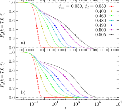
Figure 6: (Color online) Intermediate scattering functions for a series of $\phi_{\mathrm{f}}$ values at fixed $\phi_{\mathrm{m}}=0.05$ and $k=7.0$. (a) Connected correlator $F_{\mathrm{c}}(k,t)$, (b) single-particle correlator $F_{\mathrm{s}}(k,t)$. Error bars: see Fig. 2.

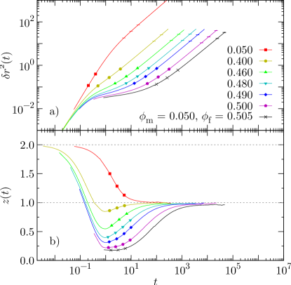
Figure 7: (Color online) Mean-squared displacement (a) and its logarithmic derivative (b) for a series of $\phi_{\mathrm{f}}$ values at fixed $\phi_{\mathrm{m}}=0.05$. Error bars [only panel (a)]: see Fig. 2.

In this subsection, as well as in Sec. III.4 and III.5, we refine our findings from Kurzidim et al. (2009) concerning $F_{\mathrm{s}}(k,t)$, $F_{\mathrm{c}}(k,t)$, and $\delta r^{2}(t)$. Additionally, we computed the logarithmic derivative

$$z(t)=\frac{d\left[{}\log\delta r^{2}(t)\right]}{d\left[{}\log t\right]}$$ (6)

which facilitates the discussion of $\delta r^{2}(t)$ since in an assumed subdiffusive law of the form $\delta r^{2}(t)\propto t^{z}$ it represents the momentary value of the power $z$. The first set of data we present for state points at various $\phi_{\mathrm{f}}$ at a common $\phi_{\mathrm{m}}=0.05$, which corresponds to a vertical line in the kinetic diagrams Fig. 4 and 5 that shall henceforth be referred to as “path I.”

In Fig. 6, the time dependence of $F_{\mathrm{c}}(k,t)$ and $F_{\mathrm{s}}(k,t)$ is depicted. For both observables, the wave vector was chosen to be $k=7.0$, which is close to the first peak in the static structure factor (cf. Fig. 2). For elevated $\phi_{\mathrm{f}}$ an intermediate-time plateau can be identified in both $F_{\mathrm{s}}(k,t)$ and $F_{\mathrm{c}}(k,t)$; as $\phi_{\mathrm{f}}$ is increased, this plateau extends to longer and longer times but does not change in height. Moreover, $F_{\mathrm{s}}(k,t)$ and $F_{\mathrm{c}}(k,t)$ decay on the same time scale as they approach this type-B transition. This is a well-known phenomenon in bulk glass formers Götze and Sjögren (1992), where the collective glass transition drives the arrest of the individual particles.

The bulklike behavior is also prevalent in $\delta r^{2}(t)$, as is evident from Fig. 7. For the lowest value of $\phi_{\mathrm{f}}$ depicted, $\delta r^{2}(t)$ crosses over directly from ballistic ($z=2$) to diffusive ($z=1$) behavior. Upon increasing $\phi_{\mathrm{f}}$ the ballistic range is followed by a distinct regime in which $\delta r^{2}(t)$ grows only very slowly, which is reflected by a drop of $z(t)$ below unity and as low as $0.15$ for the highest $\phi_{\mathrm{f}}$ considered. This is another manifestation of the cage effect (cf. Sec. I). For all such $\phi_{\mathrm{f}}$, ensuingly diffusive behavior is recovered in the long-time limit, with the time to approach $z=1$ increasing enormously with $\phi_{\mathrm{f}}$.

III.4 Path II: constant intermediate matrix density

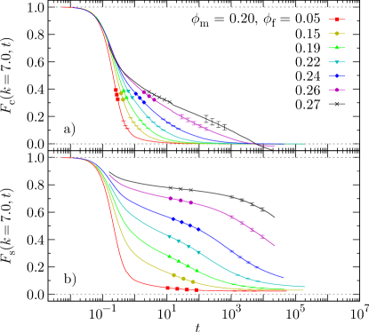
Figure 8: (Color online) Intermediate scattering functions for a series of $\phi_{\mathrm{f}}$ values at fixed $\phi_{\mathrm{m}}=0.20$ and $k=7.0$. (a) Connected correlator $F_{\mathrm{c}}(k,t)$, (b) single-particle correlator $F_{\mathrm{s}}(k,t)$. Error bars: see Fig. 2.

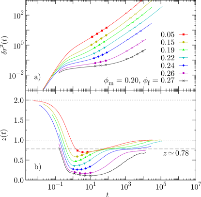
Figure 9: (Color online) Mean-squared displacement (a) and its logarithmic derivative (b) for a series of $\phi_{\mathrm{f}}$ values at fixed $\phi_{\mathrm{m}}=0.20$. Error bars [only panel (a)]: see Fig. 2.

In this subsection we present data for state points at various $\phi_{\mathrm{f}}$ at a common $\phi_{\mathrm{m}}=0.20$, i.e., along another vertical line in the kinetic diagrams presented in Sec. III.2. In the following we will refer to this line as “path II.”

In Fig. 8, the time dependence of $F_{\mathrm{c}}(k{=}7.0,t)$ and $F_{\mathrm{s}}(k{=}7.0,t)$ is depicted. As can easily be seen, the decay pattern of both correlators is quite unlike that in Sec. III.3 and Fig. 6 therein. Moreover, $F_{\mathrm{c}}(k,t)$ and $F_{\mathrm{s}}(k,t)$ deviate substantially from one another. Most strikingly, the time scales on which the correlators decay to their long-time value are vastly disparate, and increasingly so for larger values of $\phi_{\mathrm{f}}$. At $\phi_{\mathrm{f}}=0.22$, for instance, the decay times read $t_{\mathrm{c}}=7.9{\times}10^{0}$ and $t_{\mathrm{s}}=5.4{\times}10^{3}$. This represents a difference of almost three decades in time, with the collective correlator decaying faster.

$F_{\mathrm{c}}(k{=}7.0,t)$ seems to approach a transition since the time it needs to decay to its long-time value increases substantially as $\phi_{\mathrm{f}}$ is increased. However, it is difficult to pinpoint for sure whether $F_{\mathrm{c}}(k,t)$ exhibits a transition of type-A (single-step decay) or type-B (two-step decay, cf. Sec. III.3). For one, in simulations a type-A transition may show features that differ from the theoretical predictions Krakoviack (2007). Further, it is possible that an intermediate-time plateau would emerge upon increasing $\phi_{\mathrm{f}}$ above $0.27$ (the largest value of $\phi_{\mathrm{f}}$ depicted in Fig. 8). Note, however, that beyond $\phi_{\mathrm{f}}=0.27$ geometry strongly inhibits to realize system instances (see Appendix A). We conclude that using the current scheme of simulation and analysis, no definite statement can be made about the type of transition in $F_{\mathrm{c}}(k,t)$ in this part of the kinetic diagram.

$F_{\mathrm{s}}(k{=}7.0,t)$ shows an intermediate-time plateau for large values of $\phi_{\mathrm{f}}$, just as in Fig. 6. The times at which such plateau may be identified range from $10^{0}<t<10^{1}$ for $\phi_{\mathrm{f}}=0.15$ up to $10^{0}<t<10^{4}$ for $\phi_{\mathrm{f}}=0.27$. In contrast to Fig. 6, $F_{\mathrm{s}}(k,t)$ attains an additional nonzero long-time value that increases with $\phi_{\mathrm{f}}$. A tail can be identified even at the lowest fluid packing fraction considered ($\phi_{\mathrm{f}}=0.05$), whereas in this case no intermediate-time plateau is present. Therefore, for the sequence of state points at hand, two superposing decay behaviors exist in $F_{\mathrm{s}}(k,t)$: a type-A transition responsible for the long-time value, and another relaxation mechanism at higher $\phi_{\mathrm{f}}$ that leads to the intermediate-time plateau and is likely to be caused by a weak collective cage effect. The type-A transition is probably connected to the continuous diffusion-localization transition predicted by MCT Krakoviack (2009) and is discussed in more detail in Sec. III.5 and III.6.

Although not as obvious, Fig. 9 evidences that the mean-squared displacement $\delta r^{2}(t)$ differs from bulklike behavior as well. As is the case for $\phi_{\mathrm{m}}=0.05$, for $\phi_{\mathrm{m}}=0.20$ ballistic behavior is followed by a regime for which $z$ drops well below unity. Contrary to the bulklike case, this observation holds also for very low $\phi_{\mathrm{f}}$, suggesting that caging by fluid particles is not the only mechanism effective in this regime. Most likely, at low $\phi_{\mathrm{f}}$ the drop in $z$ is entirely due to the porous matrix, while at larger $\phi_{\mathrm{f}}$ both the pores and caging play a role.

For low $\phi_{\mathrm{f}}$, the range of decreasing $z$ is followed by an almost straight increase to $z=1$, i.e., a direct approach of the diffusive regime. Upon increasing $\phi_{\mathrm{f}}$, a distinct intermediate-time plateau with $z<1$ emerges in $z(t)$, which corresponds to a subdiffusive regime in $\delta r^{2}(t)$. The estimated value $z\simeq 0.78$ in the subdiffusive regime is only weakly dependent on $\phi_{\mathrm{f}}$; merely for $\phi_{\mathrm{f}}\geq 0.26$ the value of $z$ seems to systematically decrease. This decline, however, may be due to insufficient equilibration of the respective systems.

III.5 Path III: constant fluid density

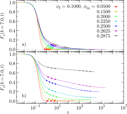
Figure 10: (Color online) Intermediate scattering functions for a series of $\phi_{\mathrm{m}}$ values at fixed $\phi_{\mathrm{f}}=0.10$ and $k=7.0$. (a) Connected correlator $F_{\mathrm{c}}(k,t)$, (b) single-particle correlator $F_{\mathrm{s}}(k,t)$. Error bars: see Fig. 2.

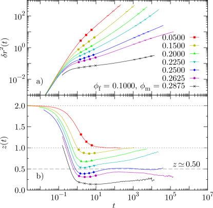
Figure 11: (Color online) Mean-squared displacement (a) and its logarithmic derivative (b) for a series of $\phi_{\mathrm{m}}$ values at fixed $\phi_{\mathrm{f}}=0.10$. Error bars [only panel (a)]: see Fig. 2.

Lastly we turn to a selection of state points at varying $\phi_{\mathrm{m}}$ for a relatively low fixed $\phi_{\mathrm{f}}=0.10$, i.e., along a horizontal straight line in the kinetic diagrams, perpendicular to paths I and II. This line will henceforth be called “path III.”

In Fig. 10 we present $F_{\mathrm{c}}(k{=}7.0,t)$ and $F_{\mathrm{s}}(k{=}7.0,t)$ for these state points. The correlators differ substantially from each other and from their bulklike counterparts—even more than was the case in Sec. III.4. Most notably, $F_{\mathrm{s}}(k,t)$ attains a sizeable nonzero value as time approaches infinity, and does so more pronouncedly as $\phi_{\mathrm{m}}$ increases. By contrast, for all $\phi_{\mathrm{m}}$ represented in Fig. 10 $F_{\mathrm{c}}(k,t)$ decays strictly to zero. On the other hand the actual pattern of the decay to the long-time value is quite similar in $F_{\mathrm{c}}(k,t)$ and $F_{\mathrm{s}}(k,t)$: unlike in Fig. 8, both correlators decay in a single step, suggesting only type-A transitions to be involved.

Comparison of Fig. 11 with Fig. 9 and 7 reveals the functional form of $\delta r^{2}(t)$ to be more sensitive to $\phi_{\mathrm{m}}$ than to $\phi_{\mathrm{f}}$. As observed in Sec. III.3, at low matrix densities the initial ballistic behavior is directly followed by diffusive behavior. For intermediate $\phi_{\mathrm{m}}<0.25$ (cf. Sec. III.4) a region of very slowly increasing particle displacement ($z<1$) succeeds the ballistic range. The value of the exponent $z$ in this region decreases as $\phi_{\mathrm{m}}$ increases. Subsequently, diffusive behavior is recovered as $z$ raises in an almost linear fashion.

Upon further increasing $\phi_{\mathrm{m}}$, at some $\phi_{\mathrm{m}}^{*}$ a geometric percolation transition takes place in the space accessible to the fluid particles (“voids”), with a void stretching through the whole system at $\phi_{\mathrm{m}}\leq\phi_{\mathrm{m}}^{*}$. This transition is intimately connected with the diffusion-localization transition predicted by MCT Krakoviack (2009) and observed in our simulations. As a hallmark of this transition, $\delta r^{2}(t)$ does not approach diffusive behavior for $\phi_{\mathrm{m}}\simeq 0.25$ but instead remains at an approximately constant $z\simeq 0.5$ for a window covering about three decades in time. Since for that matrix density $z(t)$ ultimately increases beyond $0.5$, one can expect the diffusion-localization transition to take place at slightly higher $\phi_{\mathrm{m}}$. An upper bound to that value is $\phi_{\mathrm{m}}=0.2625$, the smallest value presented that is larger than $0.25$. At this packing fraction of obstacles the window of constant $z$ extends over roughly two decades in time, with $z$ ultimately decreasing below that plateau.

Judging from these observations, the subdiffusion exponent $z$ at the diffusion-localization transition might be slightly lower than 0.5. Nevertheless, the observed value of $z$ is in striking agreement with MCT, which predicts that $z=0.5$ Krakoviack (2009). An additional agreement of numbers calls for investigation: It has long been known in theory Kärger (1992) and also verified in experiment Wei et al. (2000) that in a one-dimensional random walk—so-called “single-file diffusion”—the mean-squared displacement of the particles grows with precisely the same exponent as in our case. However, it remains an open question whether in QA systems the main effect in single-file diffusion—nonovertaking particles—is prevalent, or if other (possibly compensating) reasons lead to a coincidental agreement in $z$.

III.6 Trapping

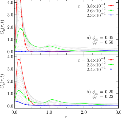
Figure 12: (Color online) self-part of the direction-averaged van Hove function $G_{\mathrm{s}}(r,t)$ for (a) $\phi_{\mathrm{m}}=0.05$, $\phi_{\mathrm{f}}=0.50$ (b) $\phi_{\mathrm{m}}=0.20$, $\phi_{\mathrm{f}}=0.22$. Curves are approximately logarithmically spaced in time; some are highlighted for visual guidance. Error bars: see Fig. 2.

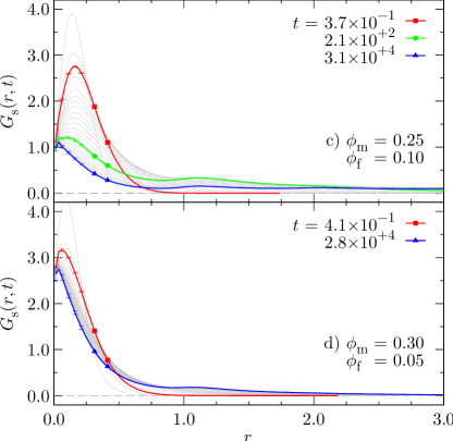
Figure 13: (Color online) self-part of the direction-averaged van Hove function $G_{\mathrm{s}}(r,t)$ for (c) $\phi_{\mathrm{m}}=0.25$, $\phi_{\mathrm{f}}=0.10$ (d) $\phi_{\mathrm{m}}=0.30$, $\phi_{\mathrm{f}}=0.05$. Curves are approximately logarithmically spaced in time; some are highlighted for visual guidance. Error bars: see Fig. 2.

In this subsection we will elucidate some aspects of the geometrical structure imposed by the quenched matrix upon the fluid immersed therein. The key concept involved is that of “voids,” i.e., domains of space that may be fully explored by a fluid particle if placed within. In HS-QA systems distinct voids are separated by infinite potential walls, and there exist voids of finite volume. Particles located in such finite void cannot travel infinitely far away from their initial location; such particles will henceforth be denoted as “trapped particles,” and the corresponding void as a “trap.” Due to the statistical nature of the matrix structure, at any nonzero matrix density there exist traps. Likewise, for any nonzero density of traps there will be trapped particles since the initial locations of the fluid particles are randomly distributed.

Two types of nontrivial questions remain to be assessed. First of all, there exists the aforementioned distinct $\phi_{\mathrm{m}}^{*}$ above which all fluid particles are trapped. Differently phrased (cf. Sec. III.5), upon varying $\phi_{\mathrm{m}}$, a percolation transition of the space accessible to the fluid particles takes place: for $\phi_{\mathrm{m}}\leq\phi_{\mathrm{m}}^{*}$, there exists an infinitely-large void, whereas for $\phi_{\mathrm{m}}>\phi_{\mathrm{m}}^{*}$ any void is of finite size. Naturally, the question arises what the precise value of $\phi_{\mathrm{m}}^{*}$ is. In the following we will investigate the behavior of fluid particles that explore the voids by studying the distribution of their displacements, as was done before for other types of confinement Höfling et al. (2006).

Our quantity of choice for the desired analysis is the self-part of the direction-averaged van Hove correlation function

$$G_{\mathrm{s}}(r,t)=\overline{\left\langle\delta\left({}r-\Delta r(t)\right)\right\rangle}$$ (7)

where $\Delta r(t)=|\mathbf{r}^{\mathrm{t}}(t)-\mathbf{r}^{\mathrm{t}}(0)|$ and by construction $\int_{0}^{\infty}G_{\mathrm{s}}(r,t)\,dr=1$. Strictly speaking, to assess the void structure only knowledge about the infinite-time limit $G_{\mathrm{s}}(r,t{\rightarrow}\infty)$ is required. However, since data are readily available, in the following we will also discuss some features of the time evolution of $G_{\mathrm{s}}(r,t)$ in order to corroborate and extend our findings from the previous sections.

Using the self-part of the van Hove function a number of quantities of interest can be assessed at least qualitatively. For instance, the matrix density at percolation, $\phi_{\mathrm{m}}^{*}$, can be estimated by exploiting the fact that as the system control parameter (here $\phi_{\mathrm{m}}$) is varied the average size of the “aggregates” (in this case the traps) diverges at the transition. For sufficiently small $r$, the distribution of trap sizes is reflected in $G_{\mathrm{s}}(r,t{\rightarrow}\infty)$ since in the infinite-time limit the nontrapped fluid particles have diffused far away. Concentrating on a particular distance $\tilde{r}\sim\sigma$, the function $G_{\mathrm{s}}(\tilde{r},t{\rightarrow}\infty;\phi_{\mathrm{m}})$ will exhibit two maxima as $\phi_{\mathrm{m}}$ is varied, one for $\phi_{\mathrm{m}}\lesssim\phi_{\mathrm{m}}^{*}$ and one for $\phi_{\mathrm{m}}\gtrsim\phi_{\mathrm{m}}^{*}$. The corresponding integral $\int_{0}^{\tilde{r}}G_{\mathrm{s}}(r,t{\rightarrow}\infty)\,dr$ represents an estimate for the fraction of fluid particles located in traps. Of course, in simulations $t{\rightarrow}\infty$ has to be approximated by some finite time $\tilde{t}$ greater than the structural relaxation time of the system.

In Fig. 12 and 13 the van Hove function is displayed at various $t$ as a function of $r$. For visual guidance, curves are highlighted for selected times. The times of successive light (gray) lines differ by ${\sim}\sqrt[6\,]{10}$, i.e., there are about six curves per time decade. In Fig. 12(a) $G_{\mathrm{s}}(r,t)$ is shown for $\phi_{\mathrm{m}}=0.05$ and $\phi_{\mathrm{f}}=0.50$, a bulklike state point like those discussed in Sec. III.3. At short times $G_{\mathrm{s}}(r,t)$ exhibits a single, approximately Gaussian peak. As $t$ increases, the maximum value of this peak decreases, but notably its $r$ position remains nearly constant even for large $t$. This is another manifestation of the cage effect prevalent in glassy systems Kob and Andersen (1995). Further support for this picture arises from the second peak in $G_{\mathrm{s}}(r,t)$ that emerges at $r\simeq 1.1$ for $t\gtrsim 10^{2}$, which indicates the presence of hopping processes. For very long times even a moderate third peak appears at $r\simeq 2$ as $G_{\mathrm{s}}(r,t)$ recovers a Gaussian-like shape centered at $r>3$.

The validity of these arguments becomes clear when considering Fig. 12(b) which depicts $G_{\mathrm{s}}(r,t)$ for $\phi_{\mathrm{m}}=0.20$ and $\phi_{\mathrm{f}}=0.22$. For this state point, representing intermediate matrix density, similar features can be observed for short and intermediate times, only with the first peak decreasing slower in height, the second peak being less pronounced, and the third peak missing. However, for large $t$ and small $r$ the shape of $G_{\mathrm{s}}(r,t)$ is markedly different from that in Fig. 12(a): even for $\tilde{t}=7.1{\times}10^{4}$ (the largest time considered) we find $G_{\mathrm{s}}(r,\tilde{t})$ to be nonzero for small $r$. Since curves of $G_{\mathrm{s}}(r,t)$ very much resemble each other for $t\lesssim\tilde{t}$ and $r<0.5$, it is reasonable to assume that in this range $G_{\mathrm{s}}(r,\tilde{t})$ represents a reliable approximation to $G_{\mathrm{s}}(r,t{\rightarrow}\infty)$. Hence we can infer the presence of trapped particles, with their fraction being $x\simeq\int_{0}^{\tilde{r}}G_{\mathrm{s}}(r,\tilde{t})\,dr=8\%$ using $\tilde{r}=0.5$. Moreover, since $G_{\mathrm{s}}(r,\tilde{t})$ is close to zero for $r>\tilde{r}$, there likely exist only few traps with a spatial extent exceeding $\tilde{r}$.

The trend seen from Fig. 12(a) to 12(b) is continued by the systems represented in Fig. 13. Panel (c) of that figure shows the state point at $\phi_{\mathrm{m}}=0.25$ and $\phi_{\mathrm{f}}=0.10$, that is, close to the diffusion-localization transition (discussed in Sec. III.5); the state point in panel (d) is situated well in the localized phase at $\phi_{\mathrm{m}}=0.30$ and $\phi_{\mathrm{f}}=0.05$. The change in shape over time becomes less pronounced as $\phi_{\mathrm{m}}$ increases, turning the second peak into a mere shoulder.

The largest times depicted in Fig. 13 again represent a sound approximation of $G_{\mathrm{s}}(r,t{\rightarrow}\infty)$. For the state point in panel (d) we numerically obtain $x\simeq\int_{0}^{\tilde{r}}G_{\mathrm{s}}(r,\tilde{t})\,dr=98\%$ using $\tilde{r}=3$ and $\tilde{t}=7.8{\times}10^{4}$, which is in excellent agreement with the figure $x=100\%$ that would be expected in an infinitely-large system residing beyond the percolation transition. For the state point in (c), using the same $\tilde{r}$ and $\tilde{t}$ we obtain $x\approx 58\%$, which, however, is rather imprecise since $G_{\mathrm{s}}(\tilde{r},\tilde{t})$ is considerably greater than zero.

In Fig. 13(c) and (d) the correlator $G_{\mathrm{s}}(r,t)$ differs markedly from that in Fig. 12(a) and (b). For one, in both (c) and (d) a second peak is present even for $t\rightarrow\infty$, suggesting that on average traps are large enough to allow for hopping. Another feature is less obvious but more important to the percolation transition: for large distances $G_{\mathrm{s}}(r,t{\rightarrow}\infty)$ is greater in (c) than in (d) for the same $r$. This implies that the mean trap size is larger in (c) than in (d), which is not unexpected—in fact this confirms the transition to take place between (b) and (d). Thus, using $G_{\mathrm{s}}(r,t)$ we find $0.22<\phi_{\mathrm{m}}^{*}<0.30$ as an estimate for the matrix packing fraction at the percolation transition, which is in accordance with our findings in the previous sections.

IV Discussion

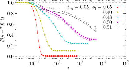
Figure 14: (Color online) Total intermediate scattering function $F(k,t)$ (lines) for selected $\phi_{\mathrm{f}}$ values at $\phi_{\mathrm{m}}=0.05$ and $k=7.0$. Symbols denote the right-hand side of Eq. (10). Error bars: see Fig. 2.

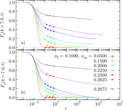
Figure 15: (Color online) self-intermediate scattering functions for a series of $\phi_{\mathrm{m}}$ values at fixed $\phi_{\mathrm{f}}=0.10$ and $k=7.0$. (a) self-correlator $F_{\mathrm{s}}(k,t)$, (b) self-correlator without long-time plateau $\tilde{F}_{\mathrm{s}}(k,t)$. For the two largest values of $\phi_{\mathrm{m}}$ in panel (b) it was not possible to reliably identify the long-time plateau. Therefore the corresponding self-correlators are left unshifted.

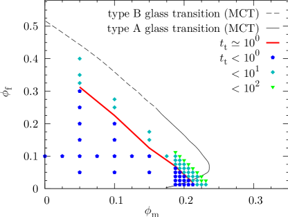
Figure 16: (Color online) Kinetic diagram based on $F(k,t)$. Symbols: time $t_{\mathrm{t}}$ needed for $F(k{=}7.0,t)$ to decay below $F^{*}=0.1$. Thick solid (red) line: interpolation through points for which $t_{\mathrm{t}}\simeq 10^{0}$.

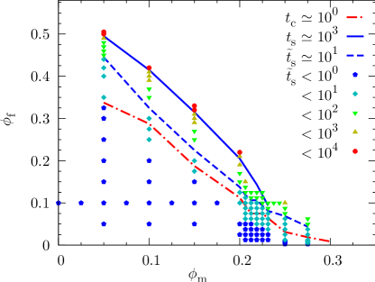
Figure 17: (Color online) Kinetic diagram based on $\tilde{F}_{\mathrm{s}}(k,t)$. Symbols: time $\tilde{t}_{\mathrm{s}}$ needed for $\tilde{F}_{\mathrm{s}}(k{=}7.0,t)$ to decay below $\tilde{F}_{\mathrm{s}}^{*}=0.1$. Dashed (blue) line: interpolation through points for which $\tilde{t}_{\mathrm{s}}\simeq 10^{1}$. Solid (blue) line: interpolation through points for which $t_{\mathrm{s}}\simeq 10^{3}$ (from Fig. 4). Dash-dotted (red) line: interpolation through points for which $t_{\mathrm{c}}\simeq 10^{0}$ (from Fig. 5).

In our presentation of the global aspects of the system’s dynamics, as well as of its behavior along selected paths in the $\{\phi_{\mathrm{m}},\phi_{\mathrm{f}}\}$ plane, we have focused our attention on self and connected density correlators as indicators of the single-particle and collective dynamics. This choice is motivated by the key role played by these dynamic correlation functions within the MCT framework for confined fluids, which provides detailed predictions for $F_{\mathrm{s}}(k,t)$ and $F_{\mathrm{c}}(k,t)$. Before discussing in more detail the comparison between the theoretical scenario of MCT and our simulations, it is instructive to study correlation functions related to $F_{\mathrm{s}}(k,t)$ and $F_{\mathrm{c}}(k,t)$. Namely, we will investigate here the total intermediate scattering function

$$F(k,t)=\frac{\overline{\left\langle\rho_{\mathbf{k}}(t)\rho_{\mathbf{-k}}(0)\right\rangle}}{S(k)}$$ (8)

as well as a modification of the self-intermediate scattering function in which the long-time plateau (as observable, for instance, along paths II and III) is subtracted out. This will allow to clarify aspects related to the kinetic diagram of the system and to facilitate the interpretation of the numerical results in the light of the MCT predictions.

By construction, fluids confined in porous media possess nonzero average density fluctuations, $\langle\rho_{\mathbf{k}}\rangle\neq 0$, induced by the matrix structure. This purely-static background becomes visible in the long-time limit of the total intermediate scattering function $F(k,t)$. Collective relaxation phenomena in confined fluids are therefore more conveniently described by the connected correlator, Eq. (5), in which only the fluctuations of the microscopic density are considered. Nevertheless it is interesting to also inspect the shape of $F(k,t)$ as a function of the state parameters. In Fig. 14 we show $F(k,t)$ for some selected densities along path I ($\phi_{\mathrm{m}}=0.05$) for the same value of $k$ considered in Fig. 6. Except for the lowest fluid density, $\phi_{\mathrm{f}}=0.05$, the $F(k,t)$ correlator attains a finite, sizeable plateau at long times. To check whether this long-time plateau is due to the purely-static background mentioned above or actually reflects a nonergodic behavior of the system, we also include in this figure the function $[S_{\mathrm{c}}(k)F_{\mathrm{c}}(k,t)+S_{\mathrm{b}}(k)]/S(k)$, where

$$S_{\mathrm{b}}(k)=\overline{\left\langle\rho_{\mathbf{k}}\right\rangle\left\langle\rho_{\mathbf{-k}}\right\rangle}$$ (9)

is the so-called blocked structure factor, and $S_{\mathrm{c}}(k)=S(k)-S_{\mathrm{b}}(k)$ is the connected structure factor. It is easy to show that, if the system is ergodic, the blocked structure factor is the infinite-time limit of the un-normalized total intermediate scattering function Krakoviack (2007) and that

$$F(k,t)=\frac{S_{\mathrm{c}}(k)F_{\mathrm{c}}(k,t)+S_{\mathrm{b}}(k)}{S(k)}$$ (10)

holds as an equality.

From Fig. 14 we see that this equality is indeed fulfilled for $\phi_{\mathrm{f}}\lesssim 0.48$, while slight deviations occur at the largest fluid packing fractions. Note, however, that the calculation of $S_{\mathrm{b}}(k)$ is also affected by statistical noise (see error bars in Fig. 14) and systematic effects Schwanzer et al. (2009). Nonetheless Eq. (10) provides an effective criterion to discriminate nonequilibrated samples as far as the collective relaxation is concerned. We also note that if we employ the criterion $F(k{=}7.0,t_{\mathrm{t}})=0.1$ to define the relaxation time $t_{\mathrm{t}}$, the latter strongly overestimates the slowness of the collective relaxations compared to $t_{\mathrm{c}}$ due to the emergence of the finite plateau in $F(k,t)$ upon increasing $\phi_{\mathrm{f}}$. This should be born in mind when discussing decoupling phenomena between single-particle and collective properties.

A similar, yet physically different long-time plateau is observed in the self-intermediate scattering functions along path II and III (see Fig. 8 and 10). As discussed in Sec. III.6, the finite value of $F_{\mathrm{s}}(k,t{\rightarrow}\infty)$ reflects the trapping of particles in disconnected voids of the matrix structure. Since the existence of a rising plateau affects the evaluation of the relaxation times $t_{\mathrm{s}}$, it is sensible to define a modified correlator $\tilde{F}_{\mathrm{s}}(k,t)=F_{\mathrm{s}}(k,t)-F_{\mathrm{s}}(k,t{\rightarrow}\infty)$, where the long-time limit $F_{\mathrm{s}}(k,t{\rightarrow}\infty)$ is identified by some construction . The results of this procedure are collected in Fig. 15 for selected state points at $\phi_{\mathrm{f}}=0.10$ (path III) and compared to the corresponding $F_{\mathrm{s}}(k,t)$. At the two largest $\phi_{\mathrm{m}}$ the relaxation to the finite plateau is not complete within the time range considered, and the correlators are left unshifted. Evaluation of the single-particle relaxation time $\tilde{t}_{\mathrm{s}}$, defined by $\tilde{F}_{\mathrm{s}}(k{=}7.0,\tilde{t}_{\mathrm{s}})=0.1$ as for the other correlators, allows to filter out the contribution to the single-particle dynamics due to trapping.

We constructed two alternative kinetic diagrams for the system at hand using the relaxation times $t_{\mathrm{t}}$ and $\tilde{t}_{\mathrm{s}}$ obtained from $F(k,t)$ and $\tilde{F}_{\mathrm{s}}(k,t)$. As in Sec. III.2, lines drawn in Fig. 16 and 17 correspond to a fixed, constant value of the relaxation times (isorelaxation times lines). Let us first focus on Fig. 16, displaying the kinetic diagram based on $t_{\mathrm{t}}$. In this case, the range of state points available to determine the isorelaxation times lines is more limited due to the incipient growth of the plateau in the region of large $\phi_{\mathrm{f}}$ and large $\phi_{\mathrm{m}}$. Nevertheless it is clear that the shape of the estimated arrest line is non-re-entrant, confirming the analysis based on the connected correlators (see Fig. 5).

A more interesting effect is observed in Fig. 17 where we show the kinetic diagram based on $\tilde{t}_{\mathrm{s}}$. For better comparison with the analysis in Sec. III.2 we also include the isorelaxation times lines obtained from the self and the connected correlators. Interestingly, the shape of the kinetic diagram for $\tilde{t}_{\mathrm{s}}$ strongly resembles that obtained from the connected correlator. In particular, the iso-$\tilde{t}_{\mathrm{s}}$ lines do not bend rapidly toward $\phi_{\mathrm{f}}=0$ as $\phi_{\mathrm{m}}$ is increased but rather stretch to larger $\phi_{\mathrm{m}}$ values, following the trend of the iso-$t_{\mathrm{c}}$ line. This effect can be understood as follows: after subtracting the long-time plateau, which is due to trapping, the residual relaxation of $F_{\mathrm{s}}(k,t)$ is governed by a weak, collective caging effect. The relaxation of $F_{\mathrm{s}}(k,t)$ toward the long-time limit occurs, in fact, on a similar time scale as the relaxation of $F_{\mathrm{c}}(k,t)$. This supports our interpretation of the complex relaxation pattern of $F_{\mathrm{s}}(k,t)$ for large matrix packing fractions (see Fig. 8) as a superposition of trapping and caging effects, and confirms the connection between the diffusion-localization transition and the appearance of a nontrivial decoupling between single-particle and collective properties Kurzidim et al. (2009).

V Conclusion

In this contribution we have investigated the dynamic properties of a fluid confined in a disordered porous matrix. In our investigations we have reduced such system to a simple QA model where the matrix is a quenched configuration of a liquid and the fluid particles equilibrate within that matrix. Both matrix and fluid particles are chosen to be hard spheres of equal size. Thus, the parameter space characterizing the system reduces to a two-dimensional plane spanned by the packing fraction of the matrix particles and that of the fluid particles. Investigations have been carried out via event-driven molecular dynamics simulations, observables were evaluated using the double-averaging recipe characteristic for QA systems. Specifically, we have evaluated the connected and the single-particle intermediate scattering functions, the mean-squared displacement, and the self-part of the van Hove function.

The data and conclusions summarized here represent a counterpart to the recently presented results obtained from a theoretical framework Krakoviack (2005, 2007, 2009). The latter approach—an extension of MCT to the QA protocol—had predicted a number of intriguing features in the kinetic diagram. Our investigations have complemented this scenario of ideal transitions, unveiling the properties of the real transitions: (i) At low matrix packing fractions we have undoubtedly confirmed the predicted type-B glass transition scenario. (ii) For intermediate matrix packing fractions we have found at least two arrest mechanisms of different nature, with the self-intermediate scattering function displaying a more complex behavior than its connected counterpart. This scenario can be rationalized as a superpositioning of the effect of trapping in disconnected voids and of a weak caging mechanism collective in nature. (iii) Varying at low fluid packing fractions the density of the matrix we found evidence for a diffusion-localization transition, reflected in the self-intermediate scattering function as well as in the mean-squared displacement and in the self-part of the van Hove function. (iv) Despite considerable effort we were unable to support the predicted re-entrant transition scenario.

In order to obtain deeper insights into the open questions we have additionally considered along path II the total intermediate scattering function, and along path III we have subtracted from the self-intermediate scattering functions the long-time plateau as there is evidence that the latter is due to trapping. Our analysis of these data supports the previously established notion of an interplay between the two phenomena dominating the arrest transition at intermediate matrix packing fractions, namely trapping and caging. Work to disentangle the effects of the latter on the dynamic correlation functions is currently underway.

Appendix A System setup details

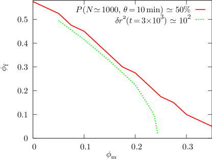
Figure 18: (Color online) Solid (red) line: probability $P(N,\theta)=50\%$ to set up a system instance with $N=N_{\mathrm{m}}{+}N_{\mathrm{f}}\simeq 1000$ particles within $\theta=10$ CPU minutes using the custom algorithm described in Appendix A. Lower left: $P(N,\theta)>50\%$, upper right: $P(N,\theta)<50\%$. Dotted (green) line: $\delta r^{2}(t)$ dynamic arrest criterion (see Sec. III.2 and Kurzidim et al. (2009)).

As mentioned in Sec. II the initial setup of a HS-QA system represents a formidable challenge. In this appendix we will point out algorithms known to succeed in setting up disordered one-component HS systems at high density, comment on problems in extending those algorithms to the QA protocol, and report on our custom solution to the problem.

The challenge is the following: Given the positions of the $N_{\mathrm{m}}$ immobile obstacle particles, permissible positions are sought for the $N_{\mathrm{f}}$ particles that during MD will be allowed to move. Unfortunately, to this respect multiple complications arise in HS-QA systems, the three most important of which are: (1) particle overlaps are strictly forbidden, (2) in the resulting configuration the matrix particles have to occupy precisely-specified locations, and (3) all voids—notably also the disconnected ones—have to be considered as locations for the fluid particles.

The simplest method—trial-and-error insertion of the fluid particles—is useless already for setting up bulk high-density systems of hard spheres. For the latter task a useful straight-forward method (although prone to crystallization) is compressing a low-density system, for instance by coordinate re-scaling combined with random particle displacements, or by applying a unidirectional force in a bounded system. However, there also exist elaborate algorithms to maximize the density in disordered HS systems; they employ for instance serial deposition Bennett (1972) or overlap elimination Jodrey and Tory (1985).

Unfortunately, the complications mentioned before render these methods difficult to adapt and/or ineffective. Therefore, in order to efficiently achieve high densities in HS-QA systems we devised a custom algorithm, which consists of the following three steps:

(1) Upon insertion of a fluid particle its “real” diameter (the diameter to be used during MD simulations) is reduced to some minute value (“deflated”) so that the probability of an insertion via trial-and-error is greatly increased. This way, throughout the search of an allowed configuration all particles can be present in the system simultaneously.

(2) In order to find such allowed configuration a simple Metropolis Monte-Carlo algorithm Metropolis et al. (1953) is employed using the HS potential. Since using this algorithm with the minute diameters is meaningless, at the beginning of each sweep (one displacement attempt for each fluid particle) the diameter of each deflated particle is increased (“inflated”) to the maximum value possible without overlapping another particle. If for a particle the latter value is greater than its real diameter then inflating is done for this particular particle and it is assigned its real diameter (“fully inflated”).

(3) A disconnected void may be filled with (almost) any number of deflated particles; however, the particular void may be too small to accommodate all of these particles if they were fully inflated. To remedy this problem, before certain sweeps all particles that are not yet fully inflated are removed from the simulation box and then re-deflated and re-inserted according to step 1. The number of sweeps separating two such removal-and-reinsertion procedures is gradually increased so as to allow for any number of sweeps to fully inflate a particle while still quickly “draining” crammed voids.

Obviously, as soon as all particles are fully inflated the setup routine is completed and a configuration fulfilling the QA requirements has been found. In step 2 the fluid particles are inflated serially. This leads to the distribution of diameters covering a wide range at all times during iteration, except when close to the approach of an allowed configuration. Since this introduces a “fluctuating polydispersity,” we found the generation of ordered states at high densities to be strongly suppressed even for bulk monodisperse systems.

Figure 18 gives an overview over the state points at which, according to the above-described steps, a system instance with $N=N_{\mathrm{m}}{+}N_{\mathrm{f}}\simeq 1000$ particles may be set up with probability $P(N,\theta)\simeq 50\%$ within $\theta=10$ CPU minutes (Intel Core 2 Duo E8400). Comparing the so-found line of discrimination (red solid line in Fig. 18) with the $\delta r^{2}(t)$ dynamic arrest criterion (green dotted line in Fig. 18; see Sec. III.2 and Kurzidim et al. (2009)) and other features of the kinetic diagrams, one can see that even using our custom routine the system setup represents a challenge to access the state points of interest.

Note that in practice a probability of 50% is unsatisfactory. Ideally, none of the setup attempts should be rejected since as little bias as possible should be exerted on the statistics. However, already at relatively low $\phi_{\mathrm{m}}$ achieving $P=100\%$ is strictly impossible, the reason being that there exist peculiar matrix configurations that prohibit all fluid particles to be inserted. Nonetheless, by prolonging the CPU time $\theta$ it is possible to increase $P$ since more theoretically possible system configurations can actually be realized. Throughout this paper only state points have been considered for which $P>90\%$ was achieved.

Appendix B Finite-size effects

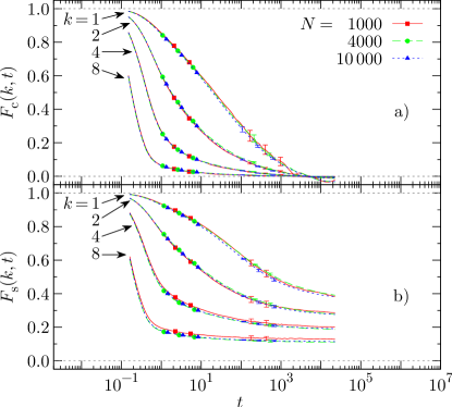
Figure 19: (Color online) Assessment of the finite-size effects present at $\phi_{\mathrm{m}}=0.2500$ and $\phi_{\mathrm{f}}=0.0125$. (a) $F_{\mathrm{c}}(k,t)$ and (b) $F_{\mathrm{s}}(k,t)$, both displayed for $k\in\{1,2,4,8\}$ as well as $N=1000$ (red solid line, squares), $N=4000$ (green dashed line, circles) and $N=10\,000$ (blue dotted line, triangles).

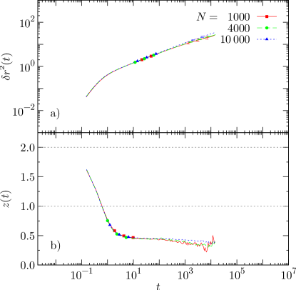
Figure 20: (Color online) Assessment of the finite-size effects present at $\phi_{\mathrm{m}}=0.2500$ and $\phi_{\mathrm{f}}=0.0125$. (a) $\delta r^{2}(t)$ and (b) $z(t)$, both displayed for $N=1000$ (red solid line, squares), $N=4000$ (green dashed line, circles) and $N=10\,000$ (blue dotted line, triangles).

As mentioned in Sec. II, throughout this work we chose to assign the same constant total number of particles $N=N_{\mathrm{m}}{+}N_{\mathrm{f}}=1000$ to most systems simulated. The purpose of this appendix is to determine for which state points this number is not sufficient to rule out the presence of finite-size effects, and to describe our pertinent solution.

Strictly adhering to the approach of constant $N$, state points with a large disparity of $\phi_{\mathrm{m}}$ and $\phi_{\mathrm{f}}$ attain low values of either $N_{\mathrm{m}}$ or $N_{\mathrm{f}}$. Neither is desirable since it will render the calculation of properties pertaining to either the matrix or the fluid inaccurate. In this work, the most extreme case for low $N_{\mathrm{m}}$ is the state point ($\phi_{\mathrm{m}}=0.050$, $\phi_{\mathrm{f}}=0.505$), with $N=1000$ entailing $N_{\mathrm{m}}=90$. The corresponding extremal case for $N_{\mathrm{f}}$ is the state point ($\phi_{\mathrm{m}}=0.3000$, $\phi_{\mathrm{f}}=0.0025$), leaving only eight fluid particles to move in a matrix of $992$ particles. Hence, in the present work the much more severe problem lies in low values of $N_{\mathrm{f}}$.

To remedy this problem we chose to adjust $N$ such that neither $N_{\mathrm{m}}$ nor $N_{\mathrm{f}}$ assume a value below a lower limit of $N^{*}=50$. The previous brief analysis shows that in none of our systems $N_{\mathrm{m}}<N^{*}$, which limits the discussion to state points with low $N_{\mathrm{f}}$. In the following, we assess whether or not the choice of $N^{*}$ is reasonable.

In order to limit the effort, we consider a single state point representative of the problem of low $N_{\mathrm{f}}$. Specifically, we inspect various observables at $\phi_{\mathrm{m}}=0.2500$ and $\phi_{\mathrm{f}}=0.0125$, i.e., at a state point close to both $\phi_{\mathrm{f}}=0$ and the percolation transition in the voids (cf. Sec. III.5 and III.6). Using $N=1000$ this system attains $N_{\mathrm{f}}=48$ which is reasonably close to $N^{*}$. To investigate finite-size effects we computed $F_{\mathrm{c}}(k,t)$, $F_{\mathrm{s}}(k,t)$, $\delta r^{2}(t)$, and $z(t)$ for $N=1000$, $4000$, and $10\,000$ while in each case averaging over ten matrix configurations.

In Fig. 19 the dependence of $F_{\mathrm{c}}(k,t;N)$ and $F_{\mathrm{s}}(k,t;N)$ upon $N$ is visualized. The intermediate scattering functions are shown for selected wave vectors, where any finite-size effects should be most prominent at small $k$. Indeed, for $k=1.0$ and $t>10^{1}$ there are noticeable discrepancies between $F_{\mathrm{c}}(k,t;N{=}1000)$, $F_{\mathrm{c}}(k,t;N{=}4000)$, and $F_{\mathrm{c}}(k,t;N{=}10\,000)$; however, this is hardly surprising considering that even for $N=10\,000$ the corresponding length scale $2\pi/k=2\pi$ is only slightly smaller than half the edge length of the simulation cell. In fact, already for $k=2$, there is no distinguishable difference between $F_{\mathrm{c}}(k,t;N{=}1000)$, $F_{\mathrm{c}}(k,t;N{=}4000)$, and $F_{\mathrm{c}}(k,t;N{=}10\,000)$. On the other hand, $F_{\mathrm{s}}(k,t;N)$ displays small consistent discrepancies between $N=1000$, $4000$, and $10\,000$; however, the worst deviation between $F_{\mathrm{s}}(k,t;N{=}1000)$ and $F_{\mathrm{s}}(k,t;N{=}10\,000)$ (which is at $k=8.0$ and $t=t_{\mathrm{max}}=2.25{\times}10^{4}$) is no more than ${\sim}12\%$. It is not surprising that the $F_{\mathrm{s}}(k,t;N)$ curves in this case exhibit larger deviations from one another than the $F_{\mathrm{c}}(k,t;N)$ curves considering that the latter approach zero rather quickly whereas $F_{\mathrm{s}}(k,t;N)$ does not completely relax. Also, we point out that any discrepancies in $F_{\mathrm{s}}(k,t;N)$ for different $N$ values are well within the range of the error bars.

Similarly, Fig. 20 illustrates the dependence of $\delta r^{2}(t;N)$ and $z(t;N)$ upon $N$. The mean-squared displacement displays only minor differences for $N=1000$, $4000$, and $10\,000$: The discrepancy between $\delta r^{2}(t;1000)$ and $\delta r^{2}(t;10\,000)$ at $t=t_{\mathrm{max}}$ amounts to ${\sim}24\%$; however, since throughout this work we are interested in $\delta r^{2}(t;N)$ on logarithmic scales, the above deviation can be considered sufficiently accurate. $z(t;N)$, on the other hand, is clearly more susceptible to stochastic errors than $\delta r^{2}(t;N)$, leading those errors to dominate finite-size effects in $z(t{>}3.6{\times}10^{3};N{=}1000)$. For $t=3.6{\times}10^{3}$, we find a difference of mere $17\%$ between $z(t;N{=}1000)$ and $z(t;N{=}10\,000)$, which permits almost quantitative interpretation.

We conclude that $N_{\mathrm{f}}=N^{*}$ is sufficient to yield reliable results for all observables considered. None of the latter exhibited a deviation of more than $20\%$ between $N=1000$ and the tenfold value for $N$, which validates all conclusions presented in this work.

References

- Gelb et al. (1999) L. D. Gelb, K. E. Gubbins, R. Radhakrishnan, and M. Sliwinska-Bartkowiak, Rep. Prog. Phys. 62, 1573 (1999).
- Rosinberg (1999) M.-L. Rosinberg, in New Approaches to Problems in Liquid State Theory, edited by C. Caccamo, J.-P. Hansen, and G. Stell (Kluwer Academic Publishers, Dordrecht, The Netherlands, 1999).
- McKenna (2000) G. B. McKenna, J. Phys. IV France 10, 343 (2000).
- McKenna (2003) G. B. McKenna, Eur. Phys. J. E 12, 191 (2003).
- Alcoutlabi and McKenna (2005) M. Alcoutlabi and G. B. McKenna, J. Phys.: Condens. Matter 17, R461 (2005).
- McKenna (2007) G. B. McKenna, Eur. Phys. J. Special Topics 141, 291 (2007).
- Madden and Glandt (1988) W. G. Madden and E. D. Glandt, J. Stat. Phys. 51, 537 (1988).
- Madden (1992) W. G. Madden, J. Chem. Phys. 96, 5422 (1992).
- Given (1992) J. A. Given, Phys. Rev. A 45, 816 (1992).
- Given and Stell (1992) J. A. Given and G. Stell, J. Chem. Phys. 97, 4573 (1992).
- Given and Stell (1994) J. A. Given and G. R. Stell, Physica A 209, 495 (1994).
- Rosinberg et al. (1994) M.-L. Rosinberg, G. Tarjus, and G. Stell, J. Chem. Phys. 100, 5172 (1994).
- Kierlik et al. (1995) E. Kierlik, M.-L. Rosinberg, G. Tarjus, and P. A. Monson, J. Chem. Phys. 103, 4256 (1995).
- Kierlik et al. (1997) E. Kierlik, M.-L. Rosinberg, G. Tarjus, and P. A. Monson, J. Chem. Phys. 106, 264 (1997).
- Paschinger and Kahl (2000) E. Paschinger and G. Kahl, Phys. Rev. E 61, 5330 (2000).
- Schöll-Paschinger et al. (2001) E. Schöll-Paschinger, D. Levesque, J.-J. Weis, and G. Kahl, Phys. Rev. E 64, 011502 (2001).
- Gallo et al. (2002) P. Gallo, R. Pellarin, and M. Rovere, EPL 57, 212 (2002).
- Gallo et al. (2003a) P. Gallo, R. Pellarin, and M. Rovere, Phys. Rev. E 67, 041202 (2003a).
- Gallo et al. (2003b) P. Gallo, R. Pellarin, and M. Rovere, Phys. Rev. E 68, 061209 (2003b).
- Kim (2003) K. Kim, EPL 61, 790 (2003).
- Höfling et al. (2006) F. Höfling, T. Franosch, and E. Frey, Phys. Rev. Lett. 96, 165901 (2006).
- Voigtmann and Horbach (2009) T. Voigtmann and J. Horbach, Phys. Rev. Lett. 103, 205901 (2009).
- Moreno and Colmenero (2006) A. J. Moreno and J. Colmenero, Phys. Rev. E 74, 021409 (2006).
- Fenz et al. (2009) W. Fenz, I. M. Mryglod, O. Prytula, and R. Folk, Phys. Rev. E 80, 021202 (2009).
- Krakoviack (2005) V. Krakoviack, Phys. Rev. Lett. 94, 065703 (2005).
- Krakoviack (2007) V. Krakoviack, Phys. Rev. E 75, 031503 (2007).
- Krakoviack (2009) V. Krakoviack, Phys. Rev. E 79, 061501 (2009).
- Chávez-Rojo et al. (2008) M. A. Chávez-Rojo, R. Juárez-Maldonado, and M. Medina-Noyola, Phys. Rev. E 77, 040401 (2008).
- Götze (1999) W. Götze, J. Phys.: Condens. Matter 11, A1 (1999).
- Götze and Sjögren (1992) W. Götze and L. Sjögren, Rep. Prog. Phys. 55, 241 (1992).
- Kurzidim et al. (2009) J. Kurzidim, D. Coslovich, and G. Kahl, Phys. Rev. Lett. 103, 138303 (2009).
- Kim et al. (2009) K. Kim, K. Miyazaki, and S. Saito, EPL 88, 36002 (2009).
- Zhang and van Tassel (2000) L. Zhang and P. R. van Tassel, J. Chem. Phys. 112, 3006 (2000).
- Zhao et al. (2006) S. L. Zhao, W. Dong, and Q. H. Liu, J. Chem. Phys. 125, 244703 (2006).
- Gallo et al. (2009) P. Gallo, A. Attili, and M. Rovere, Phys. Rev. E 80, 061502 (2009).
- Alder and Wainwright (1959) B. J. Alder and T. E. Wainwright, J. Chem. Phys. 31, 459 (1959).
- Bennett (1972) C. H. Bennett, J. Appl. Phys. 43, 2727 (1972).
- Jodrey and Tory (1985) W. S. Jodrey and E. M. Tory, Phys. Rev. A 32, 2347 (1985).
- Allen and Tildesley (1987) M. P. Allen and D. J. Tildesley, Computer Simulation of Liquids (Oxford University Press, Oxford, 1987).
- Lomba et al. (1993) E. Lomba, J. A. Given, G. Stell, J.-J. Weis, and D. Levesque, Phys. Rev. E 48, 233 (1993).
- Kob and Andersen (1995) W. Kob and H. C. Andersen, Phys. Rev. E 51, 4626 (1995).
- Hansen and McDonald (1986) J.-P. Hansen and I. R. McDonald, Theory of Simple Liquids (Elsevier Academic Press, London, 1986).
- Meroni et al. (1996) A. Meroni, D. Levesque, and J.-J. Weis, J. Chem. Phys. 105, 1101 (1996).
- Schwanzer et al. (2009) D. Schwanzer, D. Coslovich, J. Kurzidim, and G. Kahl, Mol. Phys. 107, 433 (2009).
- Kärger (1992) J. Kärger, Phys. Rev. A 45, 4173 (1992).
- Wei et al. (2000) Q.-H. Wei, C. Bechinger, and P. Leiderer, Science 287, 625 (2000).
- Metropolis et al. (1953) N. Metropolis, A. W. Rosenbluth, M. N. Rosenbluth, A. H. Teller, and E. Teller, J. Chem. Phys. 21, 1087 (1953).