Oded Schramm’s contributions to noise sensitivity

Abstract

We survey in this paper the main contributions of Oded Schramm related to noise sensitivity. We will describe in particular his various works which focused on the “spectral analysis” of critical percolation (and more generally of Boolean functions), his work on the shape-fluctuations of first passage percolation and finally his contributions to the model of dynamical percolation.

t2Supported in part by ANR-06-BLAN-00058 and the Ostrowski foundation.

A sentence which summarizes well Oded’s work on noise sensitivity is the following quote from Jean Bourgain.

There is a general philosophy which claims that if $f$ defines a property of ‘high complexity,’ then $\mathrm{Sup}\hat{f}$, the support of the Fourier Transform, has to be ‘spread out.’

Through his work on models coming from statistical physics (in particular percolation), Oded Schramm was often confronted with such functions of “high complexity.” For example, in percolation, any large-scale connectivity property can be encoded by a Boolean function of the “inputs” (edges or sites). At criticality, these large-scale connectivity functions turn out to be of “high frequency” which gives deep information on the underlying model. As we will see along this survey, Oded Schramm developed over the last decade highly original and deep ideas to understand the “complexity” of Boolean functions.

We will essentially follow the chronology of his contributions in the field; it is quite striking that three distinct periods emerge from Oded’s work and they will constitute Sections 3, 4 and 5 of this survey, corresponding, respectively, to the papers MR2001m60016 , SchrammSteif , GPS .

We have chosen to present numerous sketches of proof, since we believe that the elegance of Oded’s mathematics is best illustrated through his proofs, which usually combined imagination, simplicity and powerfulness. This choice is the reason for the length of the present survey.

[level=2]

1 Introduction.

In this Introduction, we will start by describing the scientific context in the late nineties which lead Oded Schramm to work on the sensitivity of Boolean functions. We will then motivate and define the notion of noise sensitivity and finally we will review the main contributions of Oded that will concern us throughout this survey.

1.1 Historical context.

When Oded started working on Boolean functions (with the idea to use them in statistical mechanics), there was already important literature in computer science dedicated to the properties of Boolean functions.

Here is an example of a related problem which was solved before Oded came into the field: in BenorLinial , Ben-Or and Linial conjectured that if $f$ is any Boolean function on $n$ variables (i.e., $f\dvtx\{0,1\}^{n}\to\{0,1\}$), taking the value 1 for half of the configurations of the hypercube $\{0,1\}^{n}$; then there exists some deterministic set $S=S_{f}\subset\{1,\ldots,n\}$ of less than $c\frac{n}{\log n}$ variables, such that $f$ remains undetermined as long as the variables in $S$ are not assigned (the constant $c$ being a universal constant). This means that for any such Boolean function $f$, there should always exist a set of small size which is “pivotal” for the outcome.

This conjecture was proved in KKL . Besides the proof of the conjecture, what is most striking about this paper (and which will concern us throughout the rest of this survey) is that, for the first time, techniques brought from harmonic analysis were used in KKL to study properties of Boolean functions. At the time, the authors wrote, “These new connections with harmonic analysis are very promising.”

Indeed, as they anticipated, the main technique they borrowed from harmonic analysis, namely hypercontractivity, was later used in many subsequent works. In particular, as we will see later (Section 3), hypercontractivity was one of the main ingredients in the landmark paper on noise sensitivity written by Benjamini, Kalai and Schramm MR2001m60016 .

Before going into MR2001m60016 (which introduced the concept of noise sensitivity), let us mention some of the related works in this field which appeared in the period from KKL to MR2001m60016 and which made good use of hypercontractivity. We distinguish several directions of research.

• First of all, the results of KKL have been extended to more general cases: nonbalanced Boolean functions, other measures than the uniform measure on the hypercube $\{0,1\}^{n}$ and finally, generalizations to “Boolean” functions of continuous dependence $f\dvtx[0,1]^{n}\to\{0,1\}$. See MR1194785 as well as MR1303654 . Note that both of these papers rely on hypercontractive estimates.

• Based on these generalizations, Friedgut and Kalai studied in MR1371123 the phenomenon of “sharp thresholds.” Roughly speaking, they proved that any monotone “graph property” for the so-called random graphs $G(n,p),0\leq p\leq 1$ satisfies a sharp threshold as the number of vertices $n$ goes to infinity (see MR1371123 for a more precise statement). In other words, they show that any monotone graph event $\mathcal{A}$ appears “suddenly” while increasing the edge intensity $p$ [whence a “cut-off” like shape for the function $p\mapsto{\mathbb{P}}_{n,p}(\mathcal{A})$]. In some sense their work is thus intimately related to the subject of this survey, since many examples of such “graph properties” concern connectedness, size of clusters and so on.

  The study of sharp thresholds began in percolation theory with the seminal work of Russo MR0488383 , MR671248 , where he introduced the idea of sharp thresholds in order to give an alternate proof of Kesten’s result $p_{c}(\mathbb{Z}^{2})=\frac{1}{2}$. See also the paper by Margulis MR0472604 .

• Finally, Talagrand made several remarkable contributions over this period which highly influenced Oded and his coauthors (as we will see in particular through Section 3). To name a few of these: an important result of MR2001m60016 (Theorem 3.3 in this survey) was inspired by MR1401897 ; the study of fluctuations in first passage percolation in MR2016607 (see Section 3) was influenced by a result from MR1303654 (this paper by Talagrand was already mentioned above since it somewhat overlapped with MR1194785 , MR1371123 ). More generally the questions addressed along this survey are related to the concentration of measure phenomenon which has been deeply understood by Talagrand (see MR1361756 ).

1.2 Concept of noise sensitivity.

It is now time to motivate and then define what is noise sensitivity. This concept was introduced in the seminal work MR2001m60016 whose content will be described in Section 3. As one can see from its title, noise sensitivity of Boolean functions and applications to Percolation, the authors introduced this notion having in mind applications in percolation. Before explaining these motivations in the next subsection, let us consider the following simple situation.

Assume we have some initial data $\omega=(x_{1},\ldots,x_{n})\in\{0,1\}^{n}$, and we are interested in some functional of this data that we may represent by a (real-valued) function $f\dvtx\{0,1\}^{n}\to\mathbb{R}$. Often, the functional $f$ will be the indicator function of an event $A\subset\{0,1\}^{n}$; in other words $f$ will be Boolean. Now imagine that there are some errors in the transmission of this data $\omega$ and that one receives only the sightly perturbed data $\omega^{\varepsilon}$; one would like that the quantity we are interested in, that is, $f(\omega)$, is not “too far” from what we actually receive, that is, $f(\omega^{\varepsilon})$. (A similar situation would be: we are interested in some real data $\omega$ but there are some inevitable errors in collecting this data and one ends up with $\omega^{\varepsilon}$.) To take a typical example, if $f\dvtx\{0,1\}^{n}\to\{0,1\}$ represents a voting scheme, for example, majority, then it is natural to wonder how robust $f$ is with respect to errors.

At that point, one would like to know how to properly model the perturbed data $\omega^{\varepsilon}$. The correct answer depends on the probability law which governs our “random” data $\omega$. In the rest of this survey, our data will always be sampled according to the uniform measure; hence it will be sufficient for us to assume that $\omega\sim{\mathbb{P}}={\mathbb{P}}^{n}=(\frac{1}{2}\delta_{0}+\frac{1}{2}\delta_{1})^{\otimes n}$, the uniform measure on $\{0,1\}^{n}$. Other natural measures may be considered instead, but we will stick to this simpler case. Therefore a natural way to model the perturbed data $\omega^{\varepsilon}$ is to assume that each variable in $\omega=(x_{1},\ldots,x_{n})$ is resampled independently with small probability $\varepsilon$. Equivalently, if $\omega=(x_{1},\ldots,x_{n})$, then $\omega^{\varepsilon}$ will correspond to the random configuration $(y_{1},\ldots,y_{n})$, where independently for each $i\in\{1,\ldots,n\}$, with probability $1-\varepsilon$, $y_{i}:=x_{i}$ and with probability $\varepsilon$, $y_{i}$ is sampled according to a Bernoulli ($1/2$). It is clear that such a “noising” procedure preserves the uniform measure on $\{0,1\}^{n}$.

In computer science, one is naturally interested in the noise stability of $f$ which, if $f$ is Boolean (i.e., with values in $\{0,1\}$), can be measured by the quantity ${\mathbb{P}}[{f(\omega)\neq f(\omega^{\varepsilon})}]$, where as above ${\mathbb{P}}={\mathbb{P}}^{n}$ denotes the uniform measure on $\{0,1\}^{n}$ [in fact there is a slight abuse of notation here, since ${\mathbb{P}}$ samples the coupling $(\omega,\omega^{\varepsilon})$; hence there is also some extra randomness needed for the randomization procedure]. In MajorityStablest , it is shown using Fourier analysis that in some sense, the most stable Boolean function on $\{0,1\}^{n}$ is the majority function (under reasonable assumptions which exclude dictatorship and so on).

If a functional $f$ happens to be “noise stable,” this means that very little information is lost on the outcome $f(\omega)$ knowing the “biased” information $\omega^{\varepsilon}$. Throughout this survey, we will be mainly interested in the opposite property, namely noise sensitivity. We will give precise definitions later, but roughly speaking, $f$ will be called “noise sensitive” if almost ALL information is lost on the outcome $f(\omega)$ knowing the biased information $\omega^{\varepsilon}$. This complete loss of information can be measured as follows: $f$ will be “noise sensitive” if $\operatorname{Var}[{\mathbb{E}}[{f(\omega)\mid\omega^{\varepsilon}}]]=o(1)$. It turns out that if $\operatorname{Var}(f)=O(1)$, it is equivalent to consider the correlation between $f(\omega)$ and $f(\omega^{\varepsilon})$ and equivalently, $f$ will be called “noise sensitive” if $\operatorname{Cov}(f(\omega),f(\omega^{\varepsilon}))={\mathbb{E}}[{f(\omega)f(\omega^{\varepsilon})}]-{\mathbb{E}}[{f}]^{2}=o(1)$.

Remark 1.1.

Let us point out that noise stability and noise sensitivity are two extreme situations. Imagine our functional $f$ can be decomposed as $f=f_{\mathrm{stable}}+f_{\mathrm{sens}}$, then after transmission of the data, we will keep the information on $f_{\mathrm{stable}}$ but lose the information on the other component. As such $f$ will be neither stable nor sensitive.

We will end by an example of a noise sensitive functional in the context of percolation. Let us consider a percolation configuration $\omega_{n}$ on the rescaled lattice $\frac{1}{n}\mathbb{Z}^{2}$ in the window $[0,1]^{2}$ (see Section 2.3 for background and references on percolation) at criticality $p_{c}=\frac{1}{2}$ (hence $\omega_{n}$ is sampled according to the uniform measure on $\{0,1\}^{E_{n}}$, where $E_{n}$ is the set of edges of $\frac{1}{n}\mathbb{Z}^{2}\cap[0,1]^{2}$). In Figure 1, we represented a percolation configuration $\omega_{90}$ and its noised configuration $\omega_{90}^{\varepsilon}$ with $\varepsilon=\frac{1}{10}$. In each picture, the three largest clusters are colored in red, blue and green. As is suggested from this small-scale picture, the functional giving the size of the largest cluster turns out to be asymptotically “noise sensitive”; that is, for fixed $\varepsilon>0$ when $n\to\infty$ the entire information about the largest cluster is lost from $\omega_{n}$ to $\omega_{n}^{\varepsilon}$ (even though most of the “microscopic” information is preserved).

For nice applications of the concept of noise sensitivity in the context of computer science, see MR2208732 and ODonnellThesis .

1.3 Motivations from statistical physics.

Beside the obvious motivations in computer science, there were several motivations coming from statistical physics (mostly from percolation) which lead Benjamini, Kalai and Schramm to introduce and study noise sensitivity of Boolean functions. We wish to list some of these in this subsection.

Dynamical percolation.

In “real life,” models issued from statistical physics undergo thermal agitation; consequently, their state evolves in time. For example, in the case of the Ising model, the natural dynamics associated to thermal agitation is the so-called Glauber dynamics.

In the context of percolation, a natural dynamics modeling this thermal agitation has been introduced in MR1465800 under the name of dynamical percolation (it was also invented independently by Itai Benjamini). This model is defined in a very simple way and we will describe it in detail in Section 6 (see SurveySteif for a very nice survey).

For percolation in dimension two, it is known that at criticality, there is almost surely no infinite cluster. Nevertheless, the following open question was asked back in MR1465800 : if one lets the critical percolation configuration evolve according to this dynamical percolation process, is it the case that there will exist exceptional times where an infinite cluster will appear? As we will later see, such exceptional times indeed exist. This reflects the fact that the dynamical behavior of percolation is very different from its static behavior.

Dynamical percolation is intimately related to our concept of noise sensitivity since if $(\omega_{t})$ denotes the trajectory of a dynamical percolation process, then the configuration at time $t$ is exactly a “noised” configuration of the initial configuration $\omega_{0}$ [$\omega_{t}\equiv\omega_{0}^{\varepsilon}$ with an explicit correspondence between $t$ and $\varepsilon$ (see Section 6)].

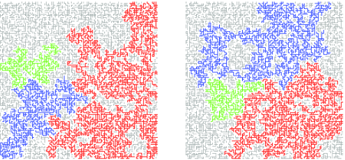
Figure 1:

As is suggested by Figure 1, large clusters of $(\omega_{t})_{t\geq 0}$ “move” (or change) very quickly as the time $t$ goes on. This rapid mixing of the large scale properties of $\omega_{t}$ is the reason for the appearance of “exceptional” infinite clusters along the dynamics. Hence, as we will see in Section 6, the above question addressed in MR1465800 needs an analysis of the noise sensitivity of large clusters. In cite MR2001m60016 , the first results in this direction are shown (they prove that in some sense any large-scale connectivity property is “noise sensitive”). However, their control on the sensitivity of large scale properties (later we will rather say the “frequency” of large-scale properties) was not sharp enough to imply that exceptional times do exist. The question was finally answered in the case of the triangular lattice in SchrammSteif thanks to a better understanding of the sensitivity of percolation. The case of $\mathbb{Z}^{2}$ was carried out in GPS . This conjecture from MR1465800 on the existence of exceptional times will be one of our driving motivations throughout this survey.

Conformal invariance of percolation.

In the nineties, an important conjecture popularized by Langlands, Pouliot and Saint-Aubin in MR1230963 stated that critical percolation should satisfy some (asymptotic) conformal invariance (in the same way as Brownian motion does). Using conformal field theory, Cardy made several important predictions based on this conformal invariance principle (see MR92m82048 ).

Conformal invariance of percolation was probably the main conjecture on planar percolation at that time and people working in this field, including Oded, were working actively on this question until Smirnov solved it on the triangular lattice in MR1851632 (note that a major motivation of the introduction of the $\mathrm{SLE}_{\kappa}$ processes by Oded in MR1776084 was this conjecture).

At the time of MR2001m60016 , conformal invariance of percolation was not yet proved (it still remains open on $\mathbb{Z}^{2}$), and the $\mathrm{SLEs}$ from MR1776084 were “in construction,” so the route toward conformal invariance was still vague. One nice idea from MR2001m60016 in this direction was to randomly perturb the lattice itself and then claim that the crossing probabilities are almost not affected by the random pertubation of the lattice. This setup is easily seen to be equivalent to proving noise sensitivity. What was difficult and remained to be done was to show that one could use such random perturbations to go from one “quad” to another conformally equivalent “quad” (see MR2001m60016 for more details). Note that at the same period, a different direction to attack conformal invariance was developed by Benjamini and Schramm in MR1646475 where they proved a certain kind of conformal invariance for Voronoï percolation.

Tsirelson’s “black noise.”

In MR1606855 , Tsirelson and Vershik constructed sigma-fields which are not “produced” by white noise (they called these sigma-fields “nonlinearizable” at that time). Tsirelson then realized that a good way to characterize a “Brownian filtration” was to test its stability versus perturbations. Systems intrinsically unstable led him to the notion of black noise (see MR2079671 for more details). This instability corresponds exactly to our notion of being “noise sensitive,” and after MR2001m60016 appeared, Tsirelson used the concept of noise sensitivity to describe his theory of black noises. Finally, black noises are related to percolation, since according to Tsirelson himself, percolation would provide the most important example of a (two-dimensional) black noise. In some sense MR2001m60016 shows that if percolation can be seen asymptotically as a noise (i.e., a continuous sigma-field which “factorizes” (see MR2079671 )), then this noise has to be black, that is, all its observables or functionals are noise sensitive. The remaining step (proving that percolation asymptotically factorizes as a noise) was proved recently by Schramm and Smirnov SSblacknoise .

Anomalous fluctuations.

In a different direction, we will see that noise sensitivity is related to the study of random shapes whose fluctuations are much smaller than “Gaussian” fluctuations (this is what we mean by “anomalous fluctuations”). Very roughly speaking, if a random metric space is highly sensitive to noise (in the sense that its geodesics are “noise sensitive”), then it induces a lot of independence within the system itself and the metric properties of the system decorrelate fast (in space or under perturbations). This instability implies in general very small fluctuations for the macroscopic metric properties (like the shape of large balls and so on). In Section 3, we will give an example of a random metric space, first passage percolation, whose fluctuations can be analyzed with the same techniques as the ones used in MR2001m60016 .

1.4 Precise definition of noise sensitivity.

Let us now fix some notations and definitions that will be used throughout the rest of the article, especially the definition of noise sensitivity which was only informal so far.

First of all, henceforth, it will be more convenient to work with the hypercube $\{-1,1\}^{n}$ rather than with $\{0,1\}^{n}$. Let us then call $\Omega_{n}:=\{-1,1\}^{n}$. The advantage of this choice is that the characters of $\{-1,1\}^{n}$ have a more simple form.

In the remainder of the text a Boolean function will denote a function from $\Omega_{n}$ into $\{0,1\}$ (except in Section 5, where when made precise it could also be into $\{-1,1\}$) and as argued above, $\Omega_{n}$ will be endowed with the uniform probability measure ${\mathbb{P}}={\mathbb{P}}^{n}$ on $\Omega_{n}$. Through this survey, we will sometimes extend the study to the larger class of real-valued functions from $\Omega_{n}$ into $\mathbb{R}$. Some of the results will hold for this larger class, but the Boolean hypothesis will be crucial at several different steps.

In the above informal discussion, “noise sensitivity” of a function $f\dvtx\Omega_{n}\to\{0,1\}$ corresponded to $\operatorname{Var}[{\mathbb{E}}[{f(\omega)\mid\omega^{\varepsilon}}]]$ or $\operatorname{Cov}(f(\omega),f(\omega^{\varepsilon}))$ being “small.” To be more specific, noise sensitivity is defined in MR2001m60016 as an asymptotic property.

Definition 1.2 (MR2001m60016 ).

Let $(m_{n})_{n\geq 0}$ be an increasing sequence in $\mathbb{N}$. A sequence of Boolean functions $f_{n}\dvtx\{-1,1\}^{m_{n}}\to\{0,1\}$ is said to be (asymptotically) noise sensitive if for any level of noise $\varepsilon>0$,

$$\operatorname{Cov}(f_{n}(\omega),f_{n}(\omega^{\varepsilon}))={\mathbb{E}}[{f_{n}(\omega)f_{n}(\omega^{\varepsilon})}]-{\mathbb{E}}[{f_{n}}]^{2}\mathop{\longrightarrow}_{n\to\infty}0.$$ (1)

In MR2001m60016 , the asymptotic condition was rather that

$$\operatorname{Var}[{\mathbb{E}}[{f_{n}(\omega)\mid\omega^{\varepsilon}}]]\-\mathop{\longrightarrow}_{n\to\infty}0,$$

but as we mentioned above, the definitions are easily seen to be equivalent (using the Fourier expansions of $f_{n}$).

Remark 1.3.

One can extend in the same fashion this definition to the class of (real-valued) functions $f_{n}\dvtx\Omega_{m_{n}}\to\mathbb{R}$ of bounded variance (bounded variance is needed to guarantee the equivalence of the two above criteria).

Remark 1.4.

Note that if $\operatorname{Var}(f_{n})$ goes to zero as $n\to\infty$, then $(f_{n})$ will automatically satisfy the condition (1), hence our definition of noise sensitivity is meaningful only for nondegenerate asymptotic events.

The opposite notion of noise stability is defined in MR2001m60016 as follows:

Definition 1.5 (MR2001m60016 ).

Let $(m_{n})_{n\geq 0}$ be an increasing sequence in $\mathbb{N}$. A sequence of Boolean functions $f_{n}\dvtx\{-1,1\}^{n}\to\{0,1\}$ is said to be (asymptotically) noise stable if

$$\sup_{n\geq 0}{\mathbb{P}}[{f_{n}(\omega)\neq f_{n}(\omega^{\varepsilon})}]\mathop{\longrightarrow}_{\varepsilon\to 0}0.$$

1.5 Structure of the paper.

In Section 2, we will review some necessary background: Fourier analysis of Boolean functions, the notion of influence and some facts about percolation. Then three Sections 3, 4 and 5, form the core of this survey. They present three different approaches, each of them enabling to localize with more or less accuracy the “frequency domain” of percolation.

The approach presented in Section 3 is based on a technique, hypercontractivity, brought from harmonic analysis. Following MR2001m60016 and MR2016607 we apply this technique to the sensitivity of percolation as well as to the study of shape fluctuations in first passage percolation. In Section 4, we describe an approach developed by Schramm and Steif in SchrammSteif based on the analysis of randomized algorithms. Section 5, following GPS , presents an approach which considers the “frequencies” of percolation as random sets in the plane; the purpose is then to study the law of these “frequencies” and to prove that they behave in some ways like random Cantor sets.

Finally, in Section 6 we present applications of the detailed information provided by the last two approaches (GPS and SchrammSteif ) to the model of dynamical percolation.

The contributions that we have chosen to present reveal personal tastes of the author. Also, the focus here is mainly on the applications in statistical mechanics and particularly percolation. Nevertheless we will try as much as possible, along this survey, to point toward other contributions Oded made close to this theme (such as MR99i60173 , MR2309980 , MR2181623 , DecisionTrees ). See also the very nice survey by Oded MR2334202 .

2 Background.

In this section, we will give some preliminaries on Boolean functions which will be used throughout the rest of the present survey. We will start with an analog of Fourier series for Boolean functions; then we will define the influence of a variable, a notion which will be particularly relevant in the remainder of the text; we will end the preliminaries section with a brief review on percolation since most of Oded’s work in noise sensitivity was motivated by applications in percolation theory.

2.1 Fourier analysis of Boolean functions.

In this survey, recall that we consider our Boolean functions as functions from the hypercube $\Omega_{n}:=\{-1,1\}^{n}$ into $\{0,1\}$, and $\Omega_{n}$ will be endowed with the uniform measure ${\mathbb{P}}={\mathbb{P}}^{n}=(\frac{1}{2}\delta_{-1}+\frac{1}{2}\delta_{1})^{\otimes n}$.

Remark 2.1.

In greater generality, one could consider other natural measures like ${\mathbb{P}}_{p}={\mathbb{P}}^{n}_{p}=((1-p)\delta_{-1}+p\delta_{1})^{\otimes n}$; these measures are relevant, for example, in the study of sharp thresholds (where one increases the “level” $p$). In the remainder of the text, it will be sufficient for us to restrict to the case of the uniform measure ${\mathbb{P}}={\mathbb{P}}_{1/2}$ on $\Omega_{n}$.

In order to apply Fourier analysis, the natural setup is to enlarge our discrete space of Boolean functions and to consider instead the larger space $L^{2}(\{-1,1\}^{n})$ of real-valued functions on $\Omega_{n}$ endowed with the inner product

$$\langle f,g\rangle:\! = \sum_{x_{1},\ldots,x_{n}}2^{-n}f(x_{1},\ldots,x_{n})g(x_{1},\ldots,x_{n})$$

$$= {\mathbb{E}}[{fg}]\qquad\mbox{for all }f,g\in L^{2}(\Omega_{n}),$$

where ${\mathbb{E}}$ denotes the expectation with respect to the uniform measure ${\mathbb{P}}$ on $\Omega_{n}$.

For any subset $S\subset\{1,2\ldots,n\}$, let $\chi_{S}$ be the function on $\{-1,1\}^{n}$ defined for any $x=(x_{1},\ldots,x_{n})$ by

$$\chi_{S}(x):=\prod_{i\in S}x_{i}.$$ (2)

It is straightforward to see that this family of $2^{n}$ functions forms an orthonormal basis of $L^{2}(\{-1,1\}^{n})$. Thus, any function $f$ on $\Omega_{n}$ (and a fortiori any Boolean function $f$) can be decomposed as

$$f=\sum_{S\subset\{1,\ldots,n\}}\hat{f}(S)\chi_{S},$$

where $\hat{f}(S)$ are the Fourier coefficients of $f$. They are sometimes called the Fourier–Walsh coefficients of $f$, and they satisfy

$$\hat{f}(S):=\langle f,\chi_{S}\rangle={\mathbb{E}}[{f\chi_{S}}].$$

Note that $\hat{f}(\varnothing)$ corresponds to the average ${\mathbb{E}}[{f}]$. As in classical Fourier analysis, if $f$ is some Boolean function, its Fourier(–Walsh) coefficients provide information on the “regularity” of $f$.

Of course one may find many other orthonormal bases for $L^{2}(\{-1,1\}^{n})$, but there are many situations for which this particular set of functions $(\chi_{S})_{S\subset\{1,\ldots,n\}}$ arises naturally. First of all there is a well-known theory of Fourier analysis on groups, a theory which is particularly simple and elegant on Abelian groups (thus including our special case of $\{-1,1\}^{n}$, but also $\mathbb{R}/\mathbb{Z}$, $\mathbb{R}$ and so on). For Abelian groups, what turns out to be relevant for doing harmonic analysis is the set $\hat{G}$ of characters of $G$ (i.e., the group homomorphisms from $G$ to $\mathbb{C}^{*}$). In our case of $G=\{-1,1\}^{n}$, the characters are precisely our functions $\chi_{S}$ indexed by $S\subset\{1,\ldots,n\}$ since they satisfy $\chi_{S}(x\cdot y)=\chi_{S}(x)\chi_{S}(y)$.

These functions also arise naturally if one performs simple random walk on the hypercube (equipped with the Hamming graph structure), since they are the eigenfunctions of the heat kernel on $\{-1,1\}^{n}$.

Last but not least, the basis $(\chi_{S})$ turns out to be particularly adapted to our study of noise sensitivity. Indeed if $f\dvtx\Omega_{n}\to\mathbb{R}$ is any real-valued function, then the correlation between $f(\omega)$ and $f(\omega^{\varepsilon})$ is nicely expressed in terms of the Fourier coefficients of $f$ as follows:

$${\mathbb{E}}[{f(\omega)f(\omega^{\varepsilon})}] = {\mathbb{E}}\biggl{[}{\biggl{(}\sum_{S_{1}}\hat{f}(S_{1})\chi_{S_{1}}(\omega)\biggr{)}\biggl{(}\sum_{S_{2}}\hat{f}(S_{2})\chi_{S_{2}}(\omega^{\varepsilon})\biggr{)}}\biggr{]}$$

$$= \sum_{S}\hat{f}(S)^{2}{\mathbb{E}}[{\chi_{S}(\omega)\chi_{S}(\omega^{\varepsilon})}]$$

$$= \sum_{S}\hat{f}(S)^{2}(1-\varepsilon)^{|S|}.$$

Therefore, the “level of sensitivity” of a Boolean function is naturally encoded in its Fourier coefficients. More precisely, for any real-valued function $f\dvtx\Omega_{n}\to\mathbb{R}$, one can consider its energy spectrum $E_{f}$ defined by

$$E_{f}(m):=\sum_{|S|=m}\hat{f}(S)^{2}\qquad\forall m\in\{1,\ldots,n\}.$$

Since $\operatorname{Cov}(f(\omega),f(\omega^{\varepsilon}))=\sum_{m=1}^{n}E_{f}(m)(1-\varepsilon)^{m}$, all the information we need is contained in the energy spectrum of $f$. As argued in the Introduction, a function of “high frequency” will be sensitive to noise while a function of “low frequency” will be stable. This allows us to give an equivalent definition of noise sensitivity (recall Definition 1.2):

Proposition 2.2

A sequence of Boolean functions $f_{n}\dvtx\{-1,1\}^{m_{n}}\to\{0,1\}$ is (asymptotically) noise sensitive if and only if, for any $k\geq 1$

$$\sum_{m=1}^{k}\sum_{|S|=m}\hat{f}_{n}(S)^{2}=\sum_{m=1}^{k}E_{f_{n}}(m)\mathop{\longrightarrow}_{n\to\infty}0.$$

Before introducing the notion of influence, let us give a simple example: Let $\Phi_{n}$ be the majority function on $n$ variables (a function which is of obvious interest in computer science). $\Phi_{n}(x_{1},\ldots,x_{n}):=\operatorname{sign}(\sum x_{i})$, where $n$ is an odd integer here. It is possible in this case to explicitly compute its Fourier coefficients, and when $n$ goes to infinity, one ends up with the following asymptotic formula (see ODonnellThesis for a nice overview and references therein):

$$E_{\Phi_{n}}(m)=\sum_{|S|=m}\widehat{\Phi_{n}}(S)^{2}=\cases{\displaystyle\frac{4}{\pi m2^{m}}\pmatrix{m-1\vspace*{2pt}\cr\dfrac{m-1}{2}}+O(m/n),&\quad if $m$ is odd,\vspace*{5pt}\cr 0,&\quad if $m$ is even.}$$

Figure 2 represents the shape of the energy spectrum of $\Phi_{n}$: its spectrum is concentrated on low frequencies which is typical

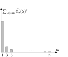
Figure 2: Spectrum of the majority function $\Phi_{n}$.

of stable functions.

Henceforth, most of this paper will be concerned with the description of the Fourier expansion of Boolean functions (and more specifically of their energy spectrum).

2.2 Notion of influence.

If $f\dvtx\Omega_{n}\to\mathbb{R}$ is a (real-valued) function, the influence of a variable $k\in[n]$ is a quantity which measures by how much (on average) the function $f$ depends on the fixed variable $k$. For this purpose, we introduce the functions

$$\nabla_{k}f\dvtx\cases{\Omega_{n}\to\mathbb{R},\cr\omega\mapsto f(\omega)-f(\sigma_{k}\cdot\omega),}\qquad\mbox{for all }k\in[n],$$

where $\sigma_{k}$ acts on $\Omega_{n}$ by flipping the $k$th bit (thus $\nabla_{k}f$ corresponds to a discrete derivative along the $k$th bit).

The influence $\mathbf{I}_{k}(f)$ of the $k$th variable is defined in terms of $\nabla_{k}f$ as follows:

$$\mathbf{I}_{k}(f):=\|\nabla_{k}f\|_{1}=\|f(\omega)-f(\sigma_{k}\cdot\omega)\|_{1}.$$

Remark 2.3.

If $f\dvtx\Omega_{n}\to\{0,1\}$ is a Boolean function corresponding to an event $A\subset\Omega_{n}$ (i.e., $f=1_{A}$), then $\mathbf{I}_{k}(f)=\mathbf{I}_{k}(A)$ is the probability that the $k$th bit is pivotal for $A$ (i.e., $\mathbf{I}_{k}(f)={\mathbb{P}}[{f(\omega)\neq f(\sigma_{k}\cdot\omega)}]$).

Remark 2.4.

If $f\dvtx\Omega_{n}\to\mathbb{R}$ is a monotone function [i.e., $f(\omega_{1})\leq f(\omega_{2})$ when $\omega_{1}\leq\omega_{2}$], then notice that

$$\hat{f}(\{k\}):={\mathbb{E}}\bigl{[}{f\chi_{\{k\}}}\bigr{]}={\mathbb{E}}[{f(x_{1},\ldots,x_{n})x_{k}}]=\tfrac 12\mathbf{I}_{k}(f)$$

by monotonicity of $f$. This gives a first hint that influences are closely related to the Fourier expansion of $f$.

We define the total influence of a (real-valued) function $f$ to be $\mathbf{I}(f):=\sum\mathbf{I}_{k}(f)$. This notion is very relevant in the study of sharp thresholds (see MR671248 , MR1371123 ). Indeed if $f$ is a monotone function, then by the Margulis–Russo formula (see, e.g., GrimmettGraphs )

$$\frac{d}{dt}\bigg{|}_{1/2}{\mathbb{P}}_{p}(f)=\mathbf{I}(f)=\sum_{k}\mathbf{I}_{k}(f).$$

This formula easily extends to all $p\in[0,1]$. In particular, for a monotone event $A$, a “large” total influence implies a “sharp” threshold for $p\mapsto{\mathbb{P}}_{p}(A)$.

As it has been recognized for quite some time already (since Ben Or/Linial), the set of all influences $\mathbf{I}_{k}(f)$, $k\in[n]$ carries important information about the function $f$. Let us then call $\operatorname{\mathbf{Inf}}(f):=(\mathbf{I}_{k}(f))_{k\in[n]}$ the influence vector of $f$. We have already seen that the $L^{1}$ norm of the influence vector encodes properties “sharp threshold”-type for $f$ since by definition $\mathbf{I}(f)=\|{\operatorname{\mathbf{Inf}}}(f)\|_{1}$. The $L^{2}$ norm of this influence vector will turn out to be a key quantity in the study of noise sensitivity of Boolean functions $f\dvtx\Omega_{n}\to\{0,1\}$. We thus define (following the notations of MR2001m60016 )

$$\mathbf{H}(f):=\sum_{k}\mathbf{I}_{k}(f)^{2}=\|{\operatorname{\mathbf{Inf}}}(f)\|_{2}^{2}.$$

For Boolean functions $f$ (i.e., with values in $\{0,1\}$), these notions [$\mathbf{I}(f)$ and $\mathbf{H}(f)$] are intimately related with the above Fourier expansion of $f$. Indeed we will see in the next section that if $f\dvtx\Omega_{n}\to\{0,1\}$, then

$$\mathbf{I}(f)=4\sum_{S}|S|\hat{f}(S)^{2}.$$

If one assumes furthermore that $f$ is monotone, then from Remark 2.4, one has

$$\frac{1}{4}\mathbf{H}(f)=\sum_{k}\hat{f}(\{k\})^{2}=\sum_{|S|=1}\hat{f}(S)^{2}=E_{f}(1),$$ (4)

which corresponds to the “weight” of the level-one Fourier coefficients [this property also holds for real-valued functions, but we will use the quantity $\mathbf{H}(f)$ only in the Boolean case].

We will conclude by the following general philosophy that we will encounter throughout the rest of the survey (especially in Section 3): if a function $f\dvtx\{0,1\}^{n}\to\mathbb{R}$ is such that each of its variables has a “very small” influence (i.e., $\ll\frac{1}{\sqrt{n}}$), then $f$ should have a behavior very different from a “Gaussian” one. We will see an illustration of this rule in the context of anomalous fluctuations (Lemma 3.9). In the Boolean case, these functions (such that all their variables have very small influence) will be noise sensitive (Theorem 3.3), which is not characteristic of Gaussian nor White noise behavior.

2.3 Fast review on percolation.

We will only briefly recall what the model is, as well as some of its properties that will be used throughout the text. For a complete account on percolation see Grimmettnewbook and more specifically in our context the lecture notes 07100856 .

We will be concerned mainly in two-dimensional percolation, and we will focus on two lattices, $\mathbb{Z}^{2}$ and the triangular lattice $\mathbb{T}$ (see Figure 3). All the results stated for $\mathbb{Z}^{2}$ in this text are also valid for percolations on “reasonable” two-dimensional translation invariant graphs for which RSW is known to hold.

Let us describe the model on $\mathbb{Z}^{2}$. Let ${\mathbb{E}}^{2}$ denote the set of edges of the graph $\mathbb{Z}^{2}$. For any $p\in[0,1]$ we define a random subgraph of $\mathbb{Z}^{2}$ as follows: independently for each edge $e\in{\mathbb{E}}^{2}$, we keep this edge with probability $p$ and remove it with probability $1-p$. Equivalently, this corresponds to defining a random configuration $\omega\in\{-1,1\}^{{\mathbb{E}}^{2}}$ where, independently for each edge $e\in{\mathbb{E}}^{2}$, we declare the edge to be open [$\omega(e)=1$] with probability $p$ or closed [$\omega(e)=-1$] with probability $1-p$. The law of the so-defined random subgraph (or configuration) is denoted by ${\mathbb{P}}_{p}$. In percolation theory, one is interested in large-scale connectivity properties of the random configuration $\omega$.

In particular as one raises the level $p$, above a certain critical parameter $p_{c}(\mathbb{Z}^{2})$, an infinite cluster (almost surely) appears. This corresponds to the well-known phase transition of percolation. By a famous theorem of Kesten this transition takes place at $p_{c}(\mathbb{Z}^{2})=\frac{1}{2}$.

Percolation is defined similarly on the triangular grid $\mathbb{T}$, except that on this lattice we will rather consider site-percolation (i.e., here we keep each site with probability $p$). Also for this model, the transition happens at the critical point $p_{c}(\mathbb{T})=\frac{1}{2}$.

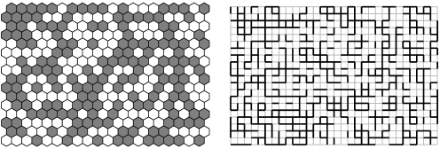
Figure 3: Illustrations by Oded representing two critical percolation configurations, respectively, on $\mathbb{T}$ and on $\mathbb{Z}^{2}$. The sites of the triangular grid are represented by hexagons.

The phase transition can be measured with the density function $\theta_{\mathbb{Z}^{2}}(p):={\mathbb{P}}_{p}(0\stackrel{{\scriptstyle\omega}}{{\longleftrightarrow}}\infty)$ which encodes important properties of the large-scale connectivities of the random configuration $\omega$: it corresponds to the density averaged over the space $\mathbb{Z}^{2}$ of the (almost surely unique) infinite cluster. The shape of the function $\theta_{\mathbb{Z}^{2}}$ is pictured in Figure 4 (notice the infinite derivative at $p_{c}$).

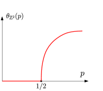
Figure 4: An illustration of the density function on $\mathbb{Z}^{2}$.

Over the last decade, the understanding of the critical regime has undergone remarkable progress, and Oded himself obviously had an enormous impact on these developments. The main ingredients of this productive period were the introduction of the $\mathrm{SLE}$ processes by Oded (see the survey on $\mathrm{SLEs}$ by Steffen Rohde in the present volume) and the proof of conformal invariance on $\mathbb{T}$ by Stanislav Smirnov MR1851632 .

At this point one cannot resist showing another famous (and everywhere used) illustration by Oded representing an exploration path on the triangular lattice (see Figure 5); this red curve which turns right on black hexagons and left on the white ones, asymptotically converges toward $\mathrm{SLE}_{6}$ (as the mesh size goes to 0).

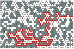
Figure 5: A sample of an exploration path on the triangular lattice.

The proof of conformal invariance combined with the detailed information given by the $\mathrm{SLE}_{6}$ process enabled one to obtain very precise information on the critical and near-critical behavior of $\mathbb{T}$-percolation. For instance, it is known that on the triangular lattice, the density function $\theta_{\mathbb{T}}(p)$ has the following behavior near $p_{c}=1/2$:

$$\theta(p)=(p-1/2)^{5/36+o(1)},$$

when $p\to 1/2+$ (see 07100856 ).

In the rest of the text, we will often rely on two types of percolation events: namely the one-arm and four-arm events. They are defined as follows: for any radius $R>1$, let $A_{R}^{1}$ be the event that the site 0 is connected to distance $R$ by some open path. Also, let $A_{R}^{4}$ be the event that there are four “arms” of alternating color from the site 0 (which can be of either color) to distance $R$ (i.e., there are four connected paths, two open, two closed from 0 to radius $R$ and the closed paths lie between the open paths). See Figure 6 for a realization of each event.

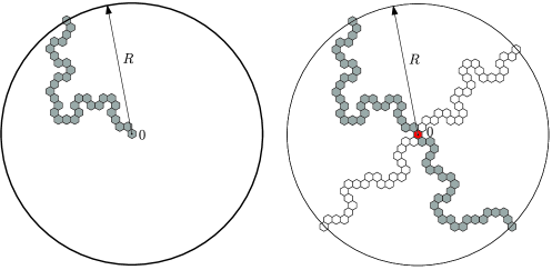
Figure 6: A realization of the one-arm event is pictured on the left; the four-arm event is pictured on the right.

It was proved in MR2002k60204 that the probability of the one-arm event decays like

$${\mathbb{P}}[{A_{R}^{1}}]:=\alpha_{1}(R)=R^{-5/{48}+o(1)}.$$

For the four-arms event, it was proved by Smirnov and Werner in MR1879816 that its probability decays like

$${\mathbb{P}}[{A_{R}^{4}}]:=\alpha_{4}(R)=R^{-5/4+o(1)}.$$

The three exponents we encountered concerning $\theta_{\mathbb{T}}$, $\alpha_{1}$ and $\alpha_{4}$ (i.e., $\frac{5}{36}$, $\frac{5}{48}$ and $\frac{5}{4}$) are known as critical exponents.

The four-arm event will be of particular importance throughout the rest of this survey. Indeed suppose the four arms event holds at some site $x\in\mathbb{T}$ up to some large distance $R$. This means that the site $x$ carries important information about the large scale connectivities within the euclidean ball $B(x,R)$. Changing the status of $x$ will drastically change the “picture” in $B(x,R)$. We call such a point a pivotal point up to distance $R$.

Finally it is often convenient to “divide” these arm-events into different scales. For this purpose, we introduce $\alpha_{4}(r,R)$ (with $r\leq R$) to be the probability that the four-arm event is realized from radius $r$ to radius $R$ [$\alpha_{1}(r,R)$ is defined similarly for the one-arm event]. By independence on disjoint sets, it is clear that if $r_{1}\leq r_{2}\leq r_{3}$ then one has $\alpha_{4}(r_{1},r_{3})\leq\alpha_{4}(r_{1},r_{2})\alpha_{4}(r_{2},r_{3})$. A very useful property known as quasi-multiplicativity claims that up to constants, these two expressions are the same (this makes the division into several scales practical). This property can be stated as follows.

Proposition 2.5 ((Quasi-multiplicativity MR88k60174 ))

For any $r_{1}\leq r_{2}\leq r_{3}$, one has (both for $\mathbb{Z}^{2}$ and $\mathbb{T}$ percolations)

$$\alpha_{4}(r_{1},r_{3})\asymp\alpha_{4}(r_{1},r_{2})\alpha_{4}(r_{2},r_{3}),$$

where the constant involved in $\asymp$ are uniform constants.

See 07100856 , NolinKesten for more details. Note also that the same property holds for the one-arm event (but is much easier to prove: it is an easy consequence of the RSW theorem which is stated in Figure 7).

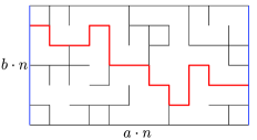
Figure 7: Left to right crossing event in a rectangle and RSW theorem.

Figure 7 represents a configuration for which the left–right crossing of $[a\cdot n$, $b\cdot n]$ is realized; in this case we define $f_{n}(\omega):=1$; otherwise we define $f_{n}(\omega):=0$. There is an extremely useful result known as RSW theorem which states that for any $a,b>0$, asymptotically the probability of crossing the rectangle ${\mathbb{P}}[{f_{n}=1}]$ remains bounded away from 0 and 1.

To end this preliminary section, let us sketch what will be one of the main goals throughout this survey: if $f_{n}$ denotes the left–right crossing event of a large rectangle $[a\cdot n,b\cdot n]$ (see Figure 7), then one can consider these observables as Boolean functions. As such they admit a Fourier expansion. Understanding the sensitivity of percolation will correspond to understanding the energy spectrum of such observables. We will see by the end of this survey that, as $n\to\infty$, the energy spectrum of $f_{n}$ should roughly look as in Figure 8.

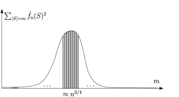
Figure 8: Expected shape of the energy spectrum of percolation crossing events. We will see in Section 5 that most of the spectral mass of $f_{n}$ is indeed localized around $n^{3/4}$. Compare this shape of the spectrum with the above spectrum of the majority function $\Phi_{n}$.

3 The “hypercontractivity” approach.

In this section, we will describe the first noise sensitivity estimates as well as anomalous fluctuations for first passage percolation (FPP).

The notion of influence will be essential throughout this section; recall that we defined $\nabla_{k}f=f-f\circ\sigma_{k}$ and $\mathbf{I}_{k}(f)=\|\nabla_{k}f\|_{1}$. It is fruitful to consider $\nabla_{k}f$ as a function from $\Omega_{n}$ into $\mathbb{R}$. Indeed, its Fourier decomposition is directly related to the Fourier decomposition of $f$ itself in the following way: it is straightforward to check that for any $S\subset[n]$

$$\widehat{\nabla_{k}f}(S)=\cases{2\hat{f}(S),&\quad if $k\in S$,\cr 0,&\quad else.}$$

If one assumes furthermore that $f$ is Boolean (i.e., $f\dvtx\Omega_{n}\to\{0,1\}$), then our discrete derivatives $\nabla_{k}f$ take their values in $\{-1,0,1\}$; this implies in particular that for any $k\in[n]$

$$\mathbf{I}_{k}(f)=\|\nabla_{k}f\|_{1}=\|\nabla_{k}f\|_{2}^{2}.$$

Using Parseval, this enables us to write the total influence of $f$ in terms of its Fourier coefficients as follows:

$$\mathbf{I}(f) = \sum_{k}\mathbf{I}_{k}(f)=\sum_{k}\|\nabla_{k}f\|_{2}^{2}$$

$$= \sum_{k}\|\widehat{\nabla_{k}f}\|_{2}^{2}$$

$$= 4\sum_{S}|S|\hat{f}(S)^{2},$$

since each “frequency” $S\subset[n]$ appears $|S|$ times. Before the appearance of the notion of “noise sensitivity” there have been several works whose focus were to get lower bounds on influences. For example (see MR1371123 ), if one wants to provide general criteria for sharp thresholds, one needs to obtain lower bounds on the total influence $\mathbf{I}(f)$. The strategy to do this in great generality was developed in KKL , where they proved that for any balanced Boolean function $f$ (balanced meaning here ${\mathbb{P}}[{f=1}]=1/2)$, there always exists a variable whose influence is greater than $O(\frac{\log n}{n})$.

Before treating in detail the case of noise sensitivity, let us describe in an informal way what was the ingenious approach from KKL to obtain lower bounds on influences. Let us consider some arbitrary balanced Boolean function $f$. We want to show that at least one of its variables has large influence $\geq c\frac{\log n}{n}$. Suppose all its influences $\mathbf{I}_{k}(f)$ are “small” (this would need to be made quantitative); this means that all the functions $\nabla_{k}f$ have small $L^{1}$ norm. Now if $f$ is Boolean (into $\{0,1\}$), then as we have noticed above, $\nabla_{k}f$ is almost Boolean (its values are in $\{-1,0,1\}$); hence $\|\nabla_{k}f\|_{1}$ being small implies that $\nabla_{k}f$ has a small support. Using the intuition coming from Weyl–Heisenberg uncertainty, $\widehat{\nabla_{k}f}$ should then be quite spread; in particular, most of its spectral mass should be concentrated on high frequencies.

This intuition (which is still vague at this point) somehow says that having small influences pushes the spectrum of $\nabla_{k}f$ toward high frequencies. Now summing up as we did in (3), but only restricting ourselves to fequencies $S$ of size smaller than some large (well-chosen) $1\ll M\ll n$, one obtains

$$\sum_{0<|S|<M}\hat{f}(S)^{2} \leq 4\sum_{0<|S|<M}|S|\hat{f}(S)^{2}$$

$$= \sum_{k}\sum_{0<|S|<M}\widehat{\nabla_{k}f}(S)^{2}$$

$$\mbox{``}\ll\mbox{''} \sum_{k}\|\widehat{\nabla_{k}f}\|_{2}^{2}$$

$$= \mathbf{I}(f),$$

where in the third line, we used the informal statement that $\widehat{\nabla_{k}f}$ should be supported on high frequencies if $f$ has small influences. Now recall that we assumed $f$ to be balanced, hence

$$\sum_{|S|>0}\hat{f}(S)^{2}=1/4.$$

Therefore, in the above equation (3), if we are in the case where a positive fraction of the Fourier mass of $f$ is concentrated below $M$, then (3) says that $\mathbf{I}(f)$ is much larger than one. In particular, at least one of the influences has to be “large.” If, on the other hand, we are in the case where most of the spectral mass of $f$ is supported on frequencies of size higher than $M$, then we also obtain that $\mathbf{I}(f)$ is large by the previous formula

$$\mathbf{I}(f)=4\sum_{S}|S|\hat{f}(S)^{2}.$$

In KKL , this intuition is converted into a proof. The main difficulty here is to formalize, or, rather, to implement, the above argument, that is, to obtain spectral information on functions with values in $\{-1,0,1\}$ knowing that they have small support. This is done KKL using techniques brought from harmonic analysis, namely hypercontractivity.

3.1 About hypercontractivity.

First, let us state what hypercontractivity corresponds to. Let $(K_{t})_{t\geq 0}$ be the heat kernel on $\mathbb{R}^{n}$. Hypercontractivity is a statement which quantifies how functions are regularized under the heat flow. The statement, which goes back to Nelson and Gross, can be simply stated as follows:

Lemma 3.1 ((Hypercontractivity))

If $1<q<2$, there is some $t=t(q)>0$ (which does not depend on the dimension $n$) such that for any $f\in L^{q}(\mathbb{R}^{n})$,

$$\|K_{t}\ast f\|_{2}\leq\|f\|_{q}.$$

The dependence $t=t(q)$ is explicit but will not concern us in the Gaussian case. Hypercontractivity is thus a regularization statement: if one starts with some initial “rough” $L^{q}$ function $f$ outside of $L^{2}$ and waits long enough [$t(q)$] under the heat flow, we end up being in $L^{2}$ with a good control on its $L^{2}$ norm.

This concept has an interesting history that is nicely explained in O’Donnell’s lectures notes (see OdonnellBlog ). It was originally invented by Nelson in MR0210416 when he needed regularization estimates on Free Fields (which are the building blocks of quantum field theory) in order to apply these in “constructive field theories.” It was then generalized by Gross in his elaboration of Logarithmic Sobolev Inequalities MR0420249 , which are an important tool in analysis. Hypercontractivity is intimately related to these Log–Sobolev inequalities (they are somewhat equivalent concepts) and thus has many applications in the theory of semi-groups, mixing of Markov chains and so on.

We now state the result in the case which concerns us, the hypercube. For any $\rho\in[0,1]$, let $T_{\rho}$ be the following “noise operator” on the functions of the hypercube: recall from the preliminary section that if $\omega\in\Omega_{n}$, we denote by $\omega^{\varepsilon}$ an $\varepsilon$-noised configuration of $\omega$. For any $f\dvtx\Omega_{n}\to\mathbb{R}$, we define $T_{\rho}f\dvtx\omega\mapsto{\mathbb{E}}[{f(\omega^{1-\rho})\mid\omega}]$. This noise operator acts in a very simple way on the Fourier coefficients

$$T_{\rho}\dvtx f=\sum_{S}\hat{f}(S)\chi_{S}\mapsto\sum_{S}\rho^{|S|}\hat{f}(S)\chi_{S}.$$

We have the following analog of Lemma 3.1:

Lemma 3.2 ((Bonami–Gross–Beckner))

For any $f\dvtx\Omega_{n}\to\mathbb{R}$,

$$\|T_{\rho}f\|_{2}\leq\|f\|_{1+\rho^{2}}.$$

The analogy with the classical Lemma 3.1 is clear: the Heat flow is replaced here by the random walk on the hypercube.

Before applying hypercontractivity to noise sensitivity, let us sketch how this functional inequality helps to implement the above idea from KKL . If a Boolean function $f$ has small influences, its discrete derivatives $\nabla_{k}f$ have small support. Now these functions have values in $\{-1,0,1\}$; thus for any $1<q<2$ we have that $\|\nabla_{k}f\|_{q}=(\|\nabla_{k}f\|_{2})^{2/q}\ll\|\nabla_{k}f\|_{2}$ (because of the small support of $\nabla_{k}f$). Now applying hypercontractivity (with $q=1+\rho^{2}$), we obtain that $\|T_{\rho}\nabla_{k}f\|_{2}\ll\|\nabla_{k}f\|_{2}$. Written on the Fourier side this means that

$$\sum_{S}\rho^{2|S|}\widehat{\nabla_{k}f}(S)^{2}\ll\sum_{S}\widehat{\nabla_{k}f}(S)^{2},$$

and this happens only if most of the spectral mass of $\nabla_{k}f$ is supported on high frequencies. It remains to make the above heuristics precise in the case which interests us here.

3.2 Applications to noise sensitivity.

Let us now see hypercontractivity in action. As in the Introduction we are interested in the noise sensitivity of a sequence of Boolean functions $f_{n}\dvtx\Omega_{m_{n}}\to\{0,1\}$. A deep theorem from MR2001m60016 can be stated as follows:

Theorem 3.3 (MR2001m60016 )

Let $(f_{n})_{n}$ be a sequence of Boolean functions. If $\mathbf{H}(f_{n})\to 0$, when $n\to\infty$, then $(f_{n})_{n}$ is noise sensitive; that is, for any $\varepsilon>0$, the correlation ${\mathbb{E}}[{f_{n}(\omega)f_{n}(\omega^{\varepsilon})}]-{\mathbb{E}}[{f}]^{2}$ converges to 0.

The theorem is true independently of the speed of convergence of $\mathbf{H}(f_{n})$. Nevertheless, if one assumes that there is some exponent $\delta>0$, such that $\mathbf{H}(f_{n})\leq(m_{n})^{-\delta}$, then the proof is quite simple as was pointed out to us by Jeff Steif, and furthermore one obtains some “logarithmic bounds” on the sensitivity of $f_{n}$. We will restrict ourselves to this stronger assumption since it will be sufficient for our application to Percolation.

Remark 3.4.

If the Boolean functions $(f_{n})_{n}$ are assumed to be monotone, it is interesting to note that as we observed in (4), $\mathbf{H}(f_{n})=\sum_{|S|=1}\hat{f}_{n}(S)^{2}$. So $\mathbf{H}(f_{n})$ corresponds here to the level-1 Fourier weights. Thus in the monotone case, Theorem 3.3 says that if asymptotically there is no weight on the level one coefficients, then there is no weight on any finite level Fourier coefficient (of course the Boolean hypothesis on $f_{n}$ is also essential here). In particular, in the monotone case, the condition $\mathbf{H}(f_{n})\to 0$ is equivalent to noise sensitivity.

Proof of Theorem 3.3 [under the stronger assumption $\mathbf{H}(f_{n})\leq(m_{n})^{-\delta}$ for some $\delta>0$] The spirit of the proof is similar to the one carried out in KKL , but the target is different here. Indeed in KKL , the goal was to obtain good lower bounds on the total influence in great generality; for example, the (easy) sharp threshold encountered by the majority function around $p=1/2$ fits into their framework. Majority is certainly not a sensitive function, so Theorem 3.3 requires more assumption than KKL results. Nevertheless the strategy will be similar: we still use the “spectral decomposition” of $f$ with respect to its “partial derivatives” $\nabla_{k}f$

$$\mathbf{I}(f)=\sum_{k}\|\nabla_{k}f\|_{2}^{2}=\sum_{k}\|\widehat{\nabla_{k}f}\|_{2}^{2}=4\sum_{S}|S|\hat{f}(S)^{2}.$$

But now we want to use the fact that $\mathbf{H}(f)=\sum_{k}\|\nabla_{k}f\|_{2}^{4}$ is very small. If $f$ is Boolean, this implies that the (almost) Boolean $\nabla_{k}f$ have very small support (and this can be made quantitative). Now, again we expect $\widehat{\nabla_{k}f}$ to be spread, but this time, we need more: not only $\nabla_{k}f$ have high frequencies, but in some sense “all their frequencies” are high leaving no mass (after summing up over the $m_{n}$ variables) to the finite level Fourier coefficients. This is implemented using hypercontractivity, following similar lines as in KKL .

Let us then consider a sequence of Boolean functions $f_{n}\dvtx\Omega_{m_{n}}\to\{0,1\}$ satisfying $\mathbf{H}(f_{n})\leq(m_{n})^{-\delta}$ for some exponent $\delta>0$. We want to show that there is some constant $M=M(\delta)$, such that

$$\sum_{0<|S|<M\log(m_{n})}\hat{f}_{n}(S)^{2}\to 0,$$

which gives a quantitative (logarithmic) noise sensitivity statement

$$\sum_{0<|S|<M\log(m_{n})}\hat{f}_{n}(S)^{2}$$

$$\qquad\leq 4\sum_{0<|S|<M\log(m_{n})}|S|\hat{f}_{n}(S)^{2}$$

$$\qquad=\sum_{k}\sum_{0<|S|<M\log(m_{n})}\widehat{\nabla_{k}f}(S)^{2}$$

$$\qquad\leq\sum_{k}\biggl{(}\frac{1}{\rho^{2}}\biggr{)}^{M\log(m_{n})}\|T_{\rho}\nabla_{k}f\|_{2}^{2}$$

$$\qquad\leq\sum_{k}\biggl{(}\frac{1}{\rho^{2}}\biggr{)}^{M\log(m_{n})}\|\nabla_{k}f\|_{1+\rho^{2}}^{2}$$

$$\eqntext{\mbox{(by hypercontractivity)}.}$$ (7)

Now, since $f$ is Boolean, one has $\|\nabla_{k}f\|_{1+\rho^{2}}=\|\nabla_{k}f\|_{2}^{2/(1+\rho^{2})}$, hence

$$\sum_{0<|S|<M\log(m_{n})}\hat{f}_{n}(S)^{2}$$

$$\qquad\leq\rho^{-2M\log(m_{n})}\sum_{k}\|\nabla_{k}f\|_{2}^{4/(1+\rho^{2})}$$

$$\qquad=\rho^{-2M\log(m_{n})}\sum_{k}\mathbf{I}_{k}(f)^{2/(1+\rho^{2})}$$

$$\qquad\leq\rho^{-2M\log(m_{n})}(m_{n})^{\rho^{2}/(1+\rho^{2})}\biggl{(}\sum_{k}\mathbf{I}_{k}(f)^{2}\biggr{)}^{1/({1+\rho^{2}})}\qquad\mbox{(By H\"{o}lder)}$$

$$\qquad=\rho^{-2M\log(m_{n})}(m_{n})^{\rho^{2}/(1+\rho^{2})}\mathbf{H}(f_{n})^{1/({1+\rho^{2}})}$$

$$\qquad\leq\rho^{-2M\log(m_{n})}(m_{n})^{({\rho^{2}-\delta})/({1+\rho^{2}})}.$$

Now by choosing $\rho\in(0,1)$ close enough to 0, and then by choosing $M=M(\delta)$ small enough, we obtain the desired logarithmic noise sensitivity.

Application to percolation. We want to apply the above result to the case of percolation crossings. Let $D$ be some smooth domain of the plane (not necessarily simply connected), and let ${\partial}_{1}$, ${\partial}_{2}$ be two smooth arcs on the boundary ${\partial}D$. For all $n\geq 1$, let $D_{n}\subset\frac{1}{n}\mathbb{Z}^{2}$ be a domain approximating $D$, and call $f_{n}$, the indicator function of a left to right crossing in $D_{n}$ from ${\partial}_{1}^{n}$ to ${\partial}_{2}^{n}$ (see Figure 9 in Section 4). Noise sensitivity of percolation means that the sequence of events $(f_{n})_{n\geq 1}$ is noise sensitive. Using Theorem 3.3, it would be enough (and necessary) to show that $\mathbf{H}(f_{n})\to 0$. But if we want a self-contained proof here, we would prefer to have at our disposal the stronger claim $\mathbf{H}(f_{n})\leq n^{-\delta}$ for some $\delta>0$ (here $m_{n}\asymp n^{2}$).

There are several ways to see why this stronger claim holds. The most natural one is to get good estimates on the probability for an edge $e$ to be pivotal. Indeed, recall that in the monotone case, $\mathbf{H}(f_{n}):=\sum_{\mathrm{edges}\ e\in D_{n}}{\mathbb{P}}[e\mbox{ is}\break\mbox{Pivotal}]^{2}$ (see Section 2.2). This probability, without considering boundary effects, is believed to be of order $n^{-5/4}$, which indeed makes $\mathbf{H}(f_{n})\approx n^{2}\cdot(n^{-5/4})^{2}\approx n^{-1/2}$ decrease to 0 polynomially fast. This behavior is now known in the case of the triangular grid thanks to Schramm’s $\mathrm{SLEs}$ and Smirnov’s proof of conformal invariance (see MR1879816 where the relevant critical exponent is computed).

At the time of MR2001m60016 , of course, critical exponents were not available (and anyway, they still remain unavailable today on $\mathbb{Z}^{2}$), but Kesten had estimates which implied that for some $\varepsilon>0$, ${\mathbb{P}}[{e\mbox{ is Pivotal}}]\leq n^{-1-\varepsilon}$ [which is enough to obtain $\mathbf{H}(f_{n})\leq n^{-\delta}$].

Furthermore, an ingenious alternative way to obtain the polynomial convergence of $\mathbf{H}(f_{n})$ was developed in MR2001m60016 which did not need Kesten’s results. This alternative way, on which we will say a few words in Section 4, in some sense prefigured the randomized algorithm approach that we will describe in the next section.

Some words on the general Theorem 3.3 and its proof. The proof of the general result is a bit more involved than the one we outlined here. The main lemma is as follows:

Lemma 3.5

There exist absolute constants $C_{k}$ for all $k\geq 1$, such that for any monotone Boolean function $f$ one has

$$\sum_{|S|=k}\hat{f}(S)^{2}\leq C_{k}\mathbf{H}(f)(-\log\mathbf{H}(f))^{k-1}.$$

This lemma “mimics” a result from Talagrand MR1401897 . Indeed Proposition 2.2 in MR1401897 can be translated as follows: for any monotone Boolean function $f$, its level-$2$ Fourier weight [i.e., $\sum_{|S|=2}\hat{f}(S)^{2}$] is bounded by $O(1)\mathbf{H}(f)\log(1/\break\mathbf{H}(f))$. It obviously implies Theorem 3.3 in the monotone case; the general case being deduced from it by a monotonization procedure. Hypercontractivity is used in the proof of this lemma.

3.3 Anomalous fluctuations, or chaos.

In this section, we will outline how hypercontractivity was used in MR2016607 in order to prove that shape fluctuations in the model of first passage percolation are sub-Gaussian.

3.3.1 The model of first passage percolation (FPP).

Let us start with the model and then state the theorem proved in MR2016607 . First passage percolation can be seen as a model of a random metric on $\mathbb{Z}^{d}$; it is defined simply as follows: independently for each edge $e\in{\mathbb{E}}^{d}$, fix the length of $e$ to be $1$ with probability $1/2$, $2$ else. In greater generality, the lengths of the edges are i.i.d. nonnegative random variables, but here, following MR2016607 , we will restrict ourselves to the above uniform distribution on $\{1,2\}$ to simplify the exposition (see MR2451057 for an extension to more general laws). In fact, in MR2016607 , they handle the slightly more general case of a uniform distribution on $\{a,b\}$ with $0<a<b$ but we decided here to stick to the case $a=1$ and $b=2$ since it makes the analogy with the previous results on influences simpler.

For any $\omega\in\{1,2\}^{{\mathbb{E}}^{d}}$, this defines a (random) metric, $\mathrm{dist}_{\omega}$, on $\mathbb{Z}^{d}$ satisfying for any $x,y\in\mathbb{Z}^{d}$,

$$\mathrm{dist}_{\omega}(x,y):=\inf_{\gamma\dvtx\mathrm{path}\ \mathrm{from}\ x\ \mathrm{to}\ y}l_{\omega}(\gamma),$$

where $l_{\omega}(\gamma)$ is the length of $\gamma$.

Using sub-additivity, it is known that the renormalized ball $\frac{1}{n}B_{\omega}(0,n)$ converges toward a deterministic shape (which can be in certain cases computed explicitly).

3.3.2 Fluctuations around the limiting shape.

The fluctuations around the asymptotic limiting shape have received tremendous interest over the last 15 years. In the two-dimensional case, using very beautiful combinatorial bijections with random matrices, certain cases of directed last passage percolation (where the law on the edges is taken to be geometric or exponential) have been understood very deeply. For example, it is known MR1737991 that the fluctuations of the ball of radius $n$ (i.e., the points whose last passage time are below $n$) around $n$ times its asymptotic deterministic shape, are of order $n^{1/3}$, and the law of these fluctuations properly renormalized follow the Tracy–Widom distribution (as do the fluctuations of the largest eigenvalue of GUE ensembles).

“Universality” is believed to hold for these models in the sense that the behavior of the fluctuations around the deterministic shape should not depend on the “microscopic” particularities of the model (e.g., the law on the edges). The shape itself does depend of course. In particular in the above model of (nondirected) first passage percolation in dimension $d=2$, fluctuations are widely believed to be also of order $n^{1/3}$ following as well the Tracy–Widom law. Still, the current state of understanding of this model is far from this conjecture.

Kesten first proved that the fluctuations of the ball of radius $n$ were at most $\sqrt{n}$ (which did not exclude yet Gaussian behavior). Benjamini, Kalai and Schramm then strengthened this result by showing that the fluctuations were sub-Gaussian. This does not yet reach the conjectured $n^{1/3}$-fluctuations, but their approach has the great advantage to be very general; in particular their result holds in any dimension $d\geq 2$.

Let us now state their main theorem concerning the fluctuations of the metric $\operatorname{dist}_{\omega}$.

Theorem 3.6 (MR2016607 )

For all $d$, there exists an absolute constant $C=C(d)$ such that in $\mathbb{Z}^{d}$

$$\operatorname{var}(\mathrm{dist}_{\omega}(0,v))\leq C\frac{|v|}{\log|v|}$$

for any point $v\in\mathbb{Z}^{2}$, $|v|\geq 2$.

3.3.3 Link with “noise sensitivity.”

This result about sub-Gaussian fluctuations might seem at first disjoint from our initial study of noise sensitivity, but they turn out to be intimately related. First of all the methods to understand one or the other, as we will see, follow very similar lines. But also, as is very nicely explained in ChatterjeeChaos , the phenomenon of “anomalous fluctuations” is in some sense equivalent to a certain “noise sensitivity” of the geodesics of first-passage-percolation. More precisely, the variance of the first passage time is of order ${\mathbb{E}}[{|\gamma(\omega(0))\cap\gamma(\omega(\tau))|}]$, where $\tau\sim\mathcal{E}(1)$ is an exponential variable. Thus we see that if the metric, or rather the geodesic, is highly perturbed when the configuration is noised; then the distances happen to be very concentrated. Chatterjee calls this phenomenon chaos. Of course, our short description here was informal since in our present setup there might be many different geodesics between two fixed points. The above link between concentration and sensitivity discovered by Chatterjee works very nicely in the context of Maxima of Gaussian processes (which in that case arise a.s. at a single point, or a single “geodesic” in a geometrical context) (see ChatterjeeChaos for more details).

3.3.4 The simpler case of the torus.

Following the approach of MR2016607 , we will first consider the case of the torus. The reason for this is that it is a much simpler case. Indeed, in the torus, for the least-passage time that we will consider, any edge will have up to constant the same influence, while in the case of $\mathrm{dist}_{\omega}(0,v)$, edges near the endpoints $0$ or $v$ have a high influence on the outcome (in some sense there is more symmetry and invariance to play with in the case of the torus).

Let $\mathbb{T}_{m}^{d}$ be the $d$-dimensional torus $(\mathbb{Z}/m\mathbb{Z})^{d}$. As in the above (lattice) model, independently for each edge of $\mathbb{T}_{m}^{d}$, we choose its length to be either $1$ or $2$. We are interested here in the smallest (random) length among closed paths $\gamma$ “turning” around the torus along the first coordinate $\mathbb{Z}/m\mathbb{Z}$ (i.e., these paths $\gamma$, once projected onto the first cycle, have winding number one). In MR2016607 , this is called the shortest circumference. For any configuration $\omega\in\{1,2\}^{E(\mathbb{T}_{m}^{d})}$, call $\operatorname{Circ}_{m}(\omega)$ this shortest circumference.

Theorem 3.7 (MR2001m60016 )

There is a constant $C>0$ (which does not depend on the dimension $d$), such that

$$\operatorname{var}(\operatorname{Circ}_{m}(\omega))\leq C\frac{m}{\log m}.$$

Remark 3.8.

A similar analysis as the one carried out below works in greater generality: if $G=(V,E)$ is some finite connected graph endowed with a random metric $d_{\omega}$ with $\omega\in\{1,2\}^{\otimes E}$, then one can obtain bounds on the fluctuation of the random diameter $D=D_{\omega}$ of $(G,d_{\omega})$. See MR2016607 , Theorem 2, for a precise statement in this more general context.

Sketch of proof of Theorem 3.7 In order to highlight the similarities with the above case of noise sensitivity of percolation, we will not follow exactly MR2016607 ; it will be more “hands-on” with the disadvantage of being less general (we take $a=1$ and $b=2$).

As before, for any edge $e$, let us consider the gradient along the edge $e$, $\nabla_{e}\operatorname{Circ}_{m}$; these gradient functions have values in $\{-1,0,1\}$, since changing the length of $e$ can only have this effect on the circumference. Note here that if the lengths of edges were in $\{a,b\}$ for any fixed choice of $0<a<b$, then it would not always be the case anymore that $\nabla_{e}\operatorname{Circ}_{m}\in\{-(b-a),0,b-a\}$. Even though this is not crucial here, this is why we stick to the case $a=1$ and $b=2$. See MR2001m60016 for a way to overcome this lack of “Boolean behavior.”

Since our gradient functions have values in $\{-1,0,1\}$, we end up being in the same setup as in our previous study; influences are defined in the same way and so on. We sill see that our gradient functions (which are “almost Boolean”) have small support, and hypercontractivity will imply the desired bounds.

Let us work in the general case of a function $f\dvtx\{-1,1\}^{n}\to\mathbb{R}$, such that for any variable $k$, $\nabla_{k}f\in\{-1,0,1\}$. We are interested in $\operatorname{var}(f)$ [and we want to show that if “influences are small” then $\operatorname{var}(f)$ is small]. It is easy to check that the variance can be written

$$\operatorname{var}(f)=\frac{1}{4}\sum_{k}\sum_{\varnothing\neq S\subset[n]}\frac{1}{|S|}\widehat{\nabla_{k}f}(S)^{2}.$$

We see on this expression, that if variables have very small influence, then as previously, the almost Boolean $\nabla_{k}f$ will be of high frequency. Heuristically, this should then imply that

$$\operatorname{var}(f) \ll \sum_{k}\sum_{S\neq\varnothing}\widehat{\nabla_{k}f}(S)^{2}$$

$$= \sum_{k}\mathbf{I}_{k}(f).$$

We prove the following lemma on the link between the fluctuations of a real-valued function $f$ on $\Omega_{n}$ and its influence vector.

Lemma 3.9

Let $f\dvtx\Omega_{n}\to\mathbb{R}$ be a (real-valued) function such that each of its discrete derivative $\nabla_{k}f,k\in[n]$ have their values in $\{-1,0,1\}$. If we assume that the influences of $f$ are small in the following sense: there exists some $\alpha>0$ such that for any $k\in\{1,\ldots,n\}$, $\mathbf{I}_{k}(f)\leq n^{-\alpha}$, then there is some constant $C=C(\alpha)$, such that

$$\operatorname{var}(f)\leq\frac{C}{\log n}\sum_{k}\mathbf{I}_{k}(f).$$

Before proving the lemma, let us see that in our special case of first passage percolation, the assumption on small influences is indeed verified. Since the edges’ length is in $\{1,2\}$, the smallest contour $\operatorname{Circ}_{m}(\omega)$ in $\mathbb{T}_{m}^{d}$ around the first coordinate lies somewhere in $[m,2m]$. Hence, if $\gamma$ is a geodesic (a path in the torus) satisfying $l(\gamma)=\operatorname{Circ}_{m}(\omega)$, then $\gamma$ uses at most $2m$ edges. There might be several different geodesics minimizing the circumference. Let us choose randomly one of these in an “invariant” way and call it $\tilde{\gamma}$. For any edge $e\in E(\mathbb{T}_{m}^{d})$, if by changing the length of $e$, the circumference increases, then $e$ has to be contained in any geodesic $\gamma$, and in particular in $\tilde{\gamma}$. This implies that ${\mathbb{P}}[{\nabla_{e}\operatorname{Circ}_{m}(\omega)>0}]\leq{\mathbb{P}}[{e\in\tilde{\gamma}}]$. By symmetry we obtain that

$${\mathbb{P}}[{\nabla_{e}\operatorname{Circ}_{m}(\omega)\neq 0}]\leq 2{\mathbb{P}}[{e\in\tilde{\gamma}}].$$

As we have seen above, $\nabla_{e}\operatorname{Circ}_{m}\in\{-1,0,1\}$; therefore $\mathbf{I}_{e}(\operatorname{Circ}_{m})\leq O(1)\times{\mathbb{P}}[{e\in\tilde{\gamma}}]$. Now using the symmetries both of the torus $\mathbb{T}_{m}^{d}$ and of our observable $\operatorname{Circ}_{m}$, if $\tilde{\gamma}$ is chosen in an appropriate invariant way (uniformly among all geodesics would work), then it is clear that all the vertical edges (the edges which, once projected on the first cycle, project on a single vertex) have the same probability to lie in $\tilde{\gamma}$; the same goes for horizontal edges. In particular,

$$\sum_{``\mathrm{vertical}\ \mathrm{edges}{{\mbox{''}}}\ e}{\mathbb{P}}[{e\in\tilde{\gamma}}]\leq{\mathbb{E}}[{|\tilde{\gamma}|}]\leq 2m.$$

Since there are $O(1)m^{d}$ vertical edges, the influence of these is bounded by $O(1)m^{1-d}$; the same goes for horizontal edges. All together this gives the desired assumption needed in Lemma 3.9. Applying this lemma, we indeed obtain that

$$\operatorname{var}(\operatorname{Circ}_{m}(\omega))\leq O(1)\frac{m}{\log m},$$

where the constant does not depend on the dimension $d$ (since the dimension helps us here). Proof of the Lemma 3.9 As for noise sensitivity, the proof relies on implementing hypercontractivity in the right way.

$$\operatorname{var}(f) = \frac{1}{4}\sum_{k}\sum_{S\neq\varnothing}\frac{1}{|S|}\widehat{\nabla_{k}f}(S)^{2}$$

$$\leq \frac{1}{4}\sum_{k}\sum_{0<|S|<c\log n}\widehat{\nabla_{k}f}(S)^{2}+\frac{O(1)}{\log n}\sum_{k}\mathbf{I}_{k}(f).$$

Hence it is enough to bound the contribution of small frequencies, $0<|S|<c\log n$, for some constant $c$ which will be chosen later. As previously we have for any $\rho\in(0,1)$ and using hypercontractivity,

$$\qquad\sum_{k}\sum_{0<|S|<c\log n}\widehat{\nabla_{k}f}(S)^{2} \leq \rho^{-2c\log n}\sum_{k}\|T_{\rho}\nabla_{k}f\|_{2}^{2}$$ (9)

$$\leq \rho^{-2c\log n}\sum_{k}\|\nabla_{k}f\|_{1+\rho^{2}}^{2}$$

$$= \rho^{-2c\log n}\sum_{k}\mathbf{I}_{k}(f)^{2/(1+\rho^{2})}$$

$$\leq \rho^{-2c\log n}\Bigl{(}\sup_{k}\mathbf{I}_{k}(f)\Bigr{)}^{({1-\rho^{2}})/({1+\rho^{2}})}\sum_{k}\mathbf{I}_{k}(f)$$

$$\leq \rho^{-2c\log n}n^{-\alpha({1-\rho^{2}})/({1+\rho^{2}})}\sum_{k}\mathbf{I}_{k}(f)$$

$$\eqntext{\mbox{(by our assumption)}.}$$

Now fixing $\rho\in(0,1)$, and then choosing the constant $c$ depending on $\rho$ and $\alpha$, the lemma follows (by optimizating on the choice of $\rho$, one could get better constants).

3.3.5 Some hints for the proof of Theorem 3.6.

The main difficulty here is that the quantity of interest, $f(\omega):=\operatorname{dist}_{\omega}(0,v)$, is not anymore invariant under a large class of graph automorphisms. This lack of symmetry makes the study of influences more difficult. (e.g., as was noticed above, edges near the endpoints 0 or $v$ will have high influence). To gain some more symmetry, the authors in MR2016607 rely on a nice “averaging” procedure. The idea is as follows: instead of looking at the (random) distance form 0 to $v$, they first pick a point $x$ randomly in the mesoscopic box $[-|v|^{1/4},|v|^{1/4}]^{d}$ around the origin and then consider the distance from this point $x$ toward $v+x$. Let $\tilde{f}$ denote this function [$\operatorname{dist}_{\omega}(x,v+x)$]. $\tilde{f}$ uses extra randomness compared to $f$, but it is clear that ${\mathbb{E}}[{f}]={\mathbb{E}}[{\tilde{f}}]$, and it is not hard to see that when $|v|$ is large, $\operatorname{var}(f)\asymp\operatorname{var}(\tilde{f})$. Therefore it is enough to study the fluctuations of the more symmetric $\tilde{f}$. (We already see here that thanks to this averaging procedure, the endpoints 0 and $v$ no longer have a high influence.) In some sense, along geodesics, this procedure “spreads” the influence on the $|v|^{1/4}$-neighborhood of the geodesics. More precisely, if $e$ is some edge, the influence of this edge is bounded by $2{\mathbb{P}}[{e\in x+\gamma}]$, where $\gamma$ is chosen among geodesics from 0 to $v$. Now, as we have seen in the case of the torus, geodesics are essentially one-dimensional [of length less than $O(1)|v|$]; this is still true on the mesoscopic scale: for any box $Q$ of radius $m:=|v|^{1/4}$, $|\gamma\cap Q|\leq O(1)m$. Now by considering the mesoscopic box around $e$, it is like moving a “line” in a box of dimension $d$; the probability for an edge to be hit by that “line” is of order $m^{1-d}$. Therefore the influence of any edge $e$ for the “spread” function $\tilde{f}$ is bounded by $O(1)|v|^{(1-d)/4}\leq O(1)|v|^{-1/4}$. This implies the needed assumption in Lemma 3.9 and hence concludes the sketch of proof of Theorem 3.7. See MR2016607 for a more detailed proof.

Remark 3.10.

In this survey, we relied on Lemma 3.9, since its proof is very similar to the noise sensitivity proof. In MR2016607 , the authors use (and reprove with better constants) an inequality from Talagrand MR1303654 which states that there is some universal constant $C>0$ such that for any $f\dvtx\{0,1\}^{n}\to\mathbb{R}$,

$$\operatorname{var}(f)\leq C\sum_{k}\frac{\|\nabla_{k}f\|_{2}^{2}}{1+\log(\|\nabla_{k}f\|_{2}/\|\nabla_{k}f\|_{1})}.\vspace*{-2pt}$$

Conclusion: Benjamini, Kalai and Schramm MR2001m60016 , MR2016607 developed multiple and very interesting techniques. The results of MR2016607 have since been extended to more general laws MR2451057 , but essentially, their control of the variance in $\Omega(n/\log n)$ is to this day still the best. The paper MR2001m60016 had a profound impact on the field. As we will see, some of the ideas present in MR2001m60016 already announced some ideas of the next section.

4 The randomized algorithm approach.

In this part, we will describe the quantitative estimates on noise sensitivity obtained in SchrammSteif . Their applications to the model of dynamical percolation will be described in the last section of this survey. But before we turn to the remarkable paper SchrammSteif , where Schramm and Steif introduced deep techniques to control Fourier spectrums of general functions, let us first mention and explain that the idea of using randomized algorithms was already present in essence in MR2001m60016 , where they used an algorithm in order to prove that $\mathbf{H}(f)$ converges quickly (polynomially) toward 0.

4.1 First appearance of randomized algorithm ideas.

In MR2001m60016 , as we have seen above, in order to prove that percolation crossings are asymptotically noise sensitive, the authors needed the fact that $\mathbf{H}(f_{n})=\sum_{k}\mathbf{I}_{k}(f_{n})^{2}\to 0$ (see Theorem 3.3); if furthermore this $L^{2}$ quantity converges to zero more quickly than a polynomial of the number of variables, $(m_{n})^{-\delta}$ for some $\delta>0$, then the proof of Theorem 3.3 is relatively simple as we outlined above. This fast convergence to zero of $\mathbf{H}(f_{n})$ was guaranteed by the work of Kesten (in particular his work MR88k60174 on hyperscaling from which follows the fact that the probability for a point to be pivotal until distance $m$ is less than $O(1)m^{-1-\alpha}$ for some $\alpha>0$).

Independently of Kesten’s approach, the authors provided in MR2001m60016 a different way of looking at this problem (an approach more in the spirit of noise sensitivity). They noticed the remarkable property that if a monotone Boolean function $f$ happens to be correlated very little with majority functions (for all subsets of the bits); then $\mathbf{H}(f)$ has to be very small, and hence the function has to be sensitive to noise. They obtained a quantitative version of this statement that we briefly state here.

Let $f\dvtx\{-1,1\}^{n}\to\{0,1\}$ be a Boolean function. We want to use its correlations with majority functions. Let us define these: for all $K\subset[n]$, define the majority function on the subset $K$ by $\mathbf{M}_{K}(x_{1},\ldots,x_{n}):=\operatorname{sign}\sum_{K}x_{i}$ (where $\operatorname{sign}0:=0$ here). The correlation of the Boolean function $f$ with these majority functions is measured by

$$\Lambda(f):={\max_{K\subset[n]}}|{\mathbb{E}}[{f\mathbf{M}_{K}}]|.$$

Being correlated very little with majority functions corresponds to $\Lambda(f)$ being very small. The following quantitative theorem about correlation with majority is proved in MR2001m60016 .

Theorem 4.1

There exists a universal constant $C>0$ such that for any $f\dvtx\Omega_{n}\to\{0,1\}$ monotone

$$\mathbf{H}(f)\leq C\Lambda(f)^{2}\bigl{(}1-\log\Lambda(f)\bigr{)}\log n$$

(the result remains valid if $f$ has values in $[0,1]$ instead).

With this result at their disposal, in order to obtain fast convergence of $\mathbf{H}(f_{n})$ to zero in the context of percolation crossings, the authors of MR2001m60016 investigated the correlations of percolation crossings $f_{n}$ with majority on subsets $K\subset[n]$. They showed that there exist $C,\alpha>0$ universal constants, so that for any subset of the lattice $K$, $|{\mathbb{E}}[{f_{n}\mathbf{M}_{K}}]|\leq Cn^{-\alpha}$. For this purpose, they used a nice appropriate randomized algorithm. We will not detail this algorithm used in MR2001m60016 , since it was considerably strengthened in SchrammSteif . We will now describe the approach of SchrammSteif and then return to “correlation with majority” using the stronger algorithm from SchrammSteif .

4.2 The Schramm/Steif approach.

The authors in SchrammSteif introduced the following beautiful and very general idea: suppose a real-valued function, $f\dvtx\Omega_{n}\to\mathbb{R}$ can be exactly computed with a randomized algorithm $A$, so that every fixed variable is used by the algorithm $A$ only with small probability; then this function $f$ has to be of “high frequency” with quantitative bounds which depend on how unlikely it is for any variable to be used by the algorithm.

4.2.1 Randomized algorithms, revealment and examples.

Let us now define more precisely what types of randomized algorithms are allowed here. Take a function $f\dvtx\{-1,1\}^{n}\to\mathbb{R}$. We are looking for algorithms which compute the output of $f$ by examining some of the bits (or variables) one by one, where the choice of the next bit may depend on the set of bits discovered so far, plus if needed, some additional randomness. We will call an algorithm satisfying this property a Markovian (randomized) algorithm. Following SchrammSteif , if $A$ is a Markovian algorithm computing the function $f$, we will denote by $J\subset[n]$ the (random) set of bits examined by the algorithm.

In order to quantify the property that variables are unlikely to be used by an algorithm $A$, we define the revealment $\bolds{\delta}=\bolds{\delta}_{A}$ of the algorithm $A$ to be the supremum over all variables $i\in[n]$ of the probability that $i$ is examined by $A$. In other words,

$$\bolds{\delta}=\bolds{\delta}_{A}=\sup_{i\in[n]}{\mathbb{P}}[{i\in J}].$$

We can now state one of the main theorems from SchrammSteif (we will sketch its proof in the next subsection).

Theorem 4.2

Let $f\dvtx\{-1,1\}^{n}\to\mathbb{R}$ be a function. Let $A$ be a Markovian randomized algorithm for $f$ having revealment $\bolds{\delta}=\bolds{\delta}_{A}$. Then for every $k=1,2,\ldots.$ The “level k”-Fourier coefficients of $f$ satisfy

$$\sum_{S\subset[n],|S|=k}\hat{f}(S)^{2}\leq\bolds{\delta}_{A}k\|f\|_{2}^{2}.$$

Remark 4.3.

If one is looking for a Markovian algorithm computing the output of the majority function on $n$ bits, then it is clear that the only way to proceed is to examine variables one at a time (the choice of the next variable being irrelevant since they all play the same role). The output will not be known until at least half of the bits are examined; hence the revealment for majority is at least $1/2$.

In the case of percolation crossings, as opposed to the above case of majority, one has to exploit the “richness” of the percolation picture in order to find algorithms which detect crossings while examining very few bits. A natural idea for a left-to-right crossing event in a large rectangle is to use an exploration path. The idea of an exploration path, which was highly influential in the Introduction by Schramm of the $\mathrm{SLE}$ processes, was pictured in Section 2.3 in the case of the triangular lattice.

More precisely, for any $n\geq 1$, let $D_{n}$ be a domain consisting of hexagons of mesh $1/n$ approximating the square $[0,1]^{2}$, or more generally any smooth “quad” $\Omega$ with two prescribed arcs ${\partial}_{1},{\partial}_{2}\subset\Omega$ (see Figure 9). We are interested in the left-to-right crossing event (in the general setting, we look at the crossing event from ${\partial}_{1}$ to ${\partial}_{2}$ in $D_{n}$). Let $f_{n}$ be the corresponding Boolean function and call $\gamma_{n}$ the “exploration path” as in Figure 9 (which starts at the upper left corner $a$). We run this exploration path until it reaches either the bottom side (in which case $f_{n}=0$) or the right-hand side (corresponding to $f_{n}=1$).

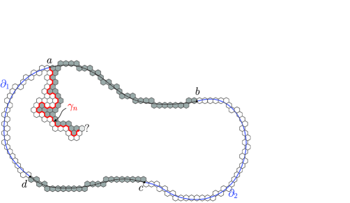
Figure 9: The random interface $\gamma_{n}$ is discovered one site at a time (which makes our algorithm Markovian). The exploration stops when $\gamma_{n}$ reaches either $(bc)$ (in which case $f_{n}=1$) or $(cd)$ ($f_{n}=0$).

This thus provides us with a Markovian algorithm to compute $f_{n}$ where the set $J=J_{n}$ of bits examined by the algorithm is the set of “hexagons” touching $\gamma_{n}$ on either side. The nice property of both the exploration path $\gamma_{n}$ and its $1/n$-neighborhood $J_{n}$, is that they have a scaling limit when the mesh $1/n$ goes to zero, this scaling limit being the well-known $\operatorname{SLE}_{6}$. (This scaling limit of the exploration path was as we mentioned above one of the main motivations of Schramm to introduce these $\operatorname{SLE}$ processes.) This scaling limit is a.s. a random fractal curve in $[0,1]^{2}$ (or $\Omega$) of Hausdorff dimension $7/4$. This means that asymptotically, the exploration path uses a very small amount of all the bits included in this picture. With some more work (see MR1879816 , 07100856 ), we can see that inside the domain (not near the corner or the sides), the probability for a point to be on $\gamma_{n}$ is of order $n^{-1/4+o(1)}$, where $o(1)$ goes to zero as the mesh goes to zero.

One therefore expects the revealment $\bolds{\delta}_{n}$ of this algorithm to be of order $n^{-1/4+o(1)}$. But the corner/boundaries have a nontrivial contribution here: for example, in this setup, the single hexagon on the upper-left corner of the domain (where the interface starts) will be used systematically by the algorithm making the revealment equal to one! There is an easy way to handle this problem: the idea in SchrammSteif is to use some additional randomness and to start the exploration path from a random point $x_{n}$ on the left-hand side of $[0,1]^{2}$. Doing so, this “smoothes” the singularity of the departure along the left boundary. There is a small counterpart to this: with this setup, one interface might not suffice to detect the existence of a left-to-right crossing, and a second interface starting from the same random point $x_{n}$ might be needed (see SchrammSteif for more details). Using arms exponents from MR1879816 and “quasimultiplicativity” of arms events MR88k60174 , SchrammSteif , it can be checked that indeed the revealment of this modified algorithm is $n^{-1/4+o(1)}$.

Theorem 4.4

Let $(f_{n})_{n\geq 1}$ be the left-to-right crossing events in domains $(D_{n})_{n\geq 1}$ approximating the unit square (or more generally a smooth domain $\Omega$). Then there exists a sequence of Markovian algorithms, whose revealments $\bolds{\delta}_{n}$ satisfy that for any $\varepsilon>0$,

$$\bolds{\delta}_{n}\leq Cn^{-1/4+\varepsilon},$$

where $C=C(\varepsilon)$ depends only on $\varepsilon$.

Therefore, applying Theorem 4.2, one obtains.

Corollary 4.5

Let $(f_{n})_{n}$ be the above sequence of crossing events. Let $\mathscr{S}_{f_{n}}$ denote the spectral sample of these Boolean functions. Since $\|f_{n}\|_{2}\leq 1$, we obtain that for any sequence $(L_{n})_{n\geq 1}$,

$${\mathbb{P}}[{0<|\mathscr{S}_{f_{n}}|<L_{n}}]\leq\bolds{\delta}_{n}L_{n}^{2}.$$ (10)

In particular, this implies that for any $\varepsilon>0$, ${\mathbb{P}}[{0<|\mathscr{S}_{f_{n}}|<n^{1/8-\varepsilon}}]\to 0$.

This result gives precise lower bound information about the “spectrum of percolation” (or its “energy spectrum”). It implies a “polynomial sensitivity” of crossing events in the sense that for any level of noise $\varepsilon_{n}\gg n^{-1/8}$, we have that ${\mathbb{E}}[{f_{n}(\omega)f_{n}(\omega^{\varepsilon_{n}})}]-{\mathbb{E}}[{f_{n}}]^{2}\to 0$.

Remark 4.6.

• Note that equation (10) gives a good control on the lower tail of the spectral distribution, and as we will see in the last section, these lower-tail estimates are essential in the study of dynamical percolation.

• Similar results are obtained by the authors in SchrammSteif in the case of the $\mathbb{Z}^{2}$-lattice, except that for this lattice, conformal invariance and convergence toward $\operatorname{SLE}_{6}$ are not known; therefore critical exponents such as $1/4$ are not available; still SchrammSteif obtains polynomial controls (thus strengthening MR2001m60016 ) but with small exponents (their value coming from RSW estimates).

4.2.2 Link with correlation with majority.

Before proving Theorem 4.2, let us briefly return to the original motivation of these types of algorithms. Suppose we have at our disposal the above Markovian Algorithms for the left-to-right crossings $f_{n}$ with small revealments $\bolds{\delta}_{n}=n^{-1/4+o(1)}$; then it follows easily that the events $f_{n}$ are mostly not correlated with majority functions; indeed let $n\geq 1$ and $K\subset D_{n}\approx[0,1]^{2}$ some fixed subset of the bits. By definition of the revealment, we have that ${\mathbb{E}}[{|K\cap J_{n}|}]\leq|K|\bolds{\delta}_{n}$. This means that on average, the algorithm visits very few variables belonging to $K$. Since

$$|{\mathbb{E}}[{f_{n}\mathbf{M}_{K}}]|=|{\mathbb{E}}[{f_{n}{\mathbb{E}}[{\mathbf{M}_{K}\mid J_{n}}]}]|\leq{\mathbb{E}}[{|{\mathbb{E}}[{\mathbf{M}_{K}\mid J_{m}}]|}],$$

and using the fact that on average, $|K\cap J_{m}|$ is small compared to $|K|$, it is easy to deduce that there is some $\alpha>0$ such that

$$\Lambda(f_{n})={\max_{K}}|{\mathbb{E}}[{f_{n}\mathbf{M}_{K}}]|\leq n^{-\alpha}.$$

This, together with Theorem 3.3 and Theorem 4.1 implies a logarithmic noise sensitivity for percolation. In MR2001m60016 , they rely on another algorithm which instead of following interfaces, in some sense “invades” clusters attached to the left-hand side. Since clusters are of fractal dimension $91/48$, intuitively their algorithm, if boundary issues can be properly taken care of, would give a bigger revealment of order $n^{-5/48+o(1)}$ (the notion of revealment only appeared in SchrammSteif ). So the major breakthrough in SchrammSteif is that they simplified tremendously the role played by the algorithm by introducing the notion of revealment and they noticed a more direct link with the Fourier transform. Using their correspondence between algorithm and spectrum, they greatly improved the control on the Fourier spectrum (polynomial v.s. logarithmic). Furthermore, they improved the randomized algorithm.

4.2.3 Proof of Theorem 4.2.

Let $f\dvtx\{-1,1\}^{n}\to\mathbb{R}$ be some real-valued function, and consider $A$, a Markovian algorithm associated to it with revealment $\bolds{\delta}=\bolds{\delta}_{A}$. Let $k\in\{1,\ldots,n\}$; we want to bound from above the size of the level-$k$ Fourier coefficients of $f$ [i.e., $\sum_{|S|=k}\hat{f}(S)^{2}$]. For this purpose, one introduces the function $g=g^{(k)}=\sum_{|S|=k}\hat{f}(S)\chi_{S}$, which is the projection of $f$ onto the subspace of level-$k$ functions. By definition, one has $\sum_{|S|=k}\hat{f}(S)^{2}=\|g\|_{2}^{2}$.

Very roughly speaking, the intuition goes as follows: if the revealment $\bolds{\delta}$ is small, then for low level $k$ there are few “frequencies” in $g^{(k)}$ which will be “seen” by the algorithm. More precisely, for any fixed “frequency” $S$, if $|S|=k$ is small, then with high probability none of the bits in $S$ will be visited by the algorithm. This means that ${\mathbb{E}}[{g^{(k)}\mid J}]$ (recall $J$ denotes the set of bits examined by the algorithm) should be of small $L^{2}$ norm compared to $g^{(k)}$. Now since $f={\mathbb{E}}[{f\mid J}]=\sum_{k}{\mathbb{E}}[{g^{(k)}\mid J}]$, most of the Fourier transform should be supported on high frequencies. There is some difficulty in implementing this intuition, since the conditional expectations ${\mathbb{E}}[{g^{(k)}\mid J}]$ are not orthogonal.

Following SchrammSteif very closely, one way to implement this idea goes as follows:

$${\mathbb{E}}[{g^{2}}]={\mathbb{E}}[{fg}]={\mathbb{E}}[{f{\mathbb{E}}[{g\mid J}]}]\leq\|f\|_{2}\|{\mathbb{E}}[{g\mid J}]\|_{2}.$$ (11)

As hinted above, the goal is to control the $L^{2}$ norm of ${\mathbb{E}}[{g\mid J}]$. In order to achieve this, it will be helpful to interpret ${\mathbb{E}}[{g\mid J}]$ as the expectation of a random function $g_{J}$ whose construction is explained below.

Recall that $J$ is the set of bits examined by the randomized algorithm $A$. Since the randomized algorithm depends on the configuration $\omega\in\{-1,1\}^{n}$ and possibly some additional randomness, one can view $J$ as a random variable on some extended probability space $\tilde{\Omega}$, whose elements can be represented as $\tilde{\omega}=(\omega,\tau)$ ($\tau$ corresponding here to the additional randomness).

For any function $h\dvtx\{-1,1\}^{n}\to\mathbb{R}$, one defines the random function $h_{J}$ which corresponds to the function $h$ where bits in $J$ are fixed to match with what was examined by the algorithm. More exactly, if $J(\tilde{\omega})=J(\omega,\tau)$ is the random set of bits examined, then the random function $h_{J}=h_{J(\tilde{\omega})}$ is the function on $\{-1,1\}^{n}$ defined by $h_{J(\omega,\tau)}(\omega^{\prime}):=h(\omega^{\prime\prime})$, where $\omega^{\prime\prime}=\omega$ on $J(\omega,\tau)$ and $\omega^{\prime\prime}=\omega^{\prime}$ on $\{1,\ldots,n\}\setminus J(\omega,\tau)$. Now, if the algorithm has examined the set of bits $J=J(\tilde{\omega})$, then with the above definition it is clear that the conditional expectation ${\mathbb{E}}[{h\mid J}]$ [which is a measurable function of $J=J(\tilde{\omega})$] corresponds to averaging $h_{J}$ over configurations $\omega^{\prime}$ [in other words we average on the variables outside of $J(\tilde{\omega})$]; this can be written as

$${\mathbb{E}}[{h\mid J}]=\int h_{J}:=\hat{h}_{J}(\varnothing),$$

where the integration $\int$ is taken with respect to the uniform measure on $\omega^{\prime}\in\Omega_{n}$. In particular ${\mathbb{E}}[{h}]={\mathbb{E}}[{\int h_{J}}]={\mathbb{E}}[{\hat{h}_{J}(\varnothing)}]$. Since $(h^{2})_{J}=(h_{J})^{2}$, it follows that

$$\|h\|_{2}^{2}={\mathbb{E}}[{h^{2}}]={\mathbb{E}}\biggl{[}{\int h_{J}^{2}}\biggr{]}={\mathbb{E}}[{\|h_{J}\|_{2}^{2}}].$$ (12)

Recall from (11) that it only remains to control $\|{\mathbb{E}}[{g\mid J}]\|_{2}^{2}={\mathbb{E}}[{\hat{g}_{J}(\varnothing)^{2}}]$. For this purpose, we apply Parseval to the (random) function $g_{J}$: this gives (for any $\tilde{\omega}\in\tilde{\Omega}$),

$$\hat{g}_{J}(\varnothing)^{2}=\|g_{J}\|_{2}^{2}-\sum_{|S|>0}\hat{g}_{J}(S)^{2}.$$

Taking the expectation over $\tilde{\omega}=(\omega,\tau)\in\tilde{\Omega}$, this leads to:

$${\mathbb{E}}[{\hat{g}_{J}(\varnothing)^{2}}] = {\mathbb{E}}[{\|g_{J}\|_{2}^{2}}]-\sum_{|S|>0}{\mathbb{E}}[{\hat{g}_{J}(S)^{2}}]$$

$$= \|g\|_{2}^{2}-\sum_{|S|>0}{\mathbb{E}}[{\hat{g}_{J}(S)^{2}}]\qquad\mbox{[by (\ref{e.hJ})]}$$

$$= \sum_{|S|=k}\hat{g}(S)^{2}-\sum_{|S|>0}{\mathbb{E}}[{\hat{g}_{J}(S)^{2}}]\qquad\cases{\mbox{since $g$ is supported}\cr\mbox{on level-$k$ coefficients}}$$

$$\leq \sum_{|S|=k}{\mathbb{E}}[{\hat{g}(S)^{2}-\hat{g}_{J}(S)^{2}}]\qquad\cases{\mbox{by restricting on}\cr\mbox{level-$k$ coefficients}.}$$

Now, since $g_{J}$ is built randomly from $g$ by fixing the variables in $J=J(\tilde{\omega})$, and since $g$ by definition does not have frequencies larger than $k$, it is clear that

$$\hat{g}_{J}(S)=\cases{\hat{g}(S)=\hat{f}(S),&\quad if $S\cap J(\tilde{\omega})=\varnothing$,\cr 0,&\quad else.}$$

Therefore, we obtain

$$\|{\mathbb{E}}[{g\mid J}]\|_{2}^{2}={\mathbb{E}}[{\hat{g}_{J}(\varnothing)^{2}}]\leq\sum_{|S|=k}\hat{g}(S)^{2}{\mathbb{P}}[{S\cap J\neq\varnothing}]\leq\|g\|_{2}^{2}k\bolds{\delta}.$$

Combining with (11), this proves Theorem 4.2.

4.3 Is there any better algorithm?

One might wonder whether there exist better algorithms which detect left-to-right crossings (better in the sense of smaller revealment). The existence of such algorithms would immediately imply sharper concentration results for the “Fourier spectrum of percolation” than in Corollary 4.5.

This question of the “most effective” algorithm is very natural and has already been addressed in another paper of Oded et al. MR2309980 , where they study random turn hex. Roughly speaking the “best” algorithm might be close to the following: assume $j$ bits (forming the set $S_{j}$) have been explored so far; then choose for the next bit to be examined, the bit having the highest chance to be pivotal for the left–right crossing conditionally on what was previously examined ($S_{j}$). This algorithm stated in this way does not require additional randomness. Hence one would need to randomize it in some way in order to have a chance to obtain a small revealment. It is clear that this algorithm (following pivotal locations) in some sense is “smarter” than the one above, but on the other hand its analysis is highly nontrivial. It is not clear to guess what the revealment for that algorithm would be.

Before turning to the next section, let us observe that even if we had at our disposal the most effective algorithm (in terms of revealment), it would not yet necessarily imply the expected concentration behavior of the spectral measure of $f_{n}$ around its mean (which for an $n\times n$ box on $\mathbb{T}$ turns out to be of order $n^{3/4}$). Indeed, in an $n\times n$ box, the algorithm will stop once it has found a crossing from left to right OR a dual crossing from top to bottom. In either case, the lattice or dual path is at least of length $n$; therefore we always have $|J|=|J_{n}|\geq n$. But if $\bolds{\delta}_{n}$ is the revealment of any algorithm computing $f_{n}$, then by definition of the revealment, one has ${\mathbb{E}}[{|J_{n}|}]\leq O(1)n^{2}\bolds{\delta}_{n}$ [there are $O(1)n^{2}$ variables]; since $|J_{n}|\geq n$, this implies that $\bolds{\delta}_{n}$ is necessarily bigger than $O(1)n^{-1}$. Now by Corollary 4.5, one has that

$$\sum_{0<|S|<n^{\alpha}}\hat{f}_{n}(S)^{2}\leq n^{2\alpha}\bolds{\delta}_{n}.$$

Therefore, the restriction that $\bolds{\delta}_{n}$ has to be bigger than $O(1)n^{-1}$ implies that with the above algorithmic approach, one cannot hope to control the Fourier tail of percolation above $n^{1/2+o(1)}$ (while as we will see in the next section, the spectral measure of $f_{n}$ is concentrated around $n^{3/4}$).

The above discussion raises the natural question of finding good lower bounds on the “revealment of percolation crossings.” It turns out that one can obtain much better lower bounds on the smallest possible revealment than the straightforward one obtained above. In our present case (percolation crossings), the best known lower bound on the revealment follows from the following theorem by O’Donnell and Servedio.

Theorem 4.7 (MR2341918 )

Let $f\dvtx\Omega_{n}\to\{-1,1\}$ be a monotone Boolean function. Any randomized algorithm $A$ which computes $f$ satisfies the following:

$$\bolds{\delta}_{A}\geq\frac{\mathbf{I}(f)^{2}}{n}=\frac{(\sum_{k}\mathbf{I}_{k}(f))^{2}}{n}.$$

In our case, $f_{n}$ depends on $O(n^{2})$ variables, and if we are on the triangular grid $\mathbb{T}$, the total influence is known to be of order $n^{3/4+o(1)}$. Hence the above theorem implies that

$$\bolds{\delta}_{n}\geq n^{-1/2+o(1)}.$$

Note that one could have recovered this lower bound also from the case $k=1$ in Theorem 4.2. Now, using Corollary 4.5, this lower bound shows that one cannot hope to obtain concentration results on $\hat{f}_{n}$ above level $n^{1/4+o(1)}$. Note that this is still far from the expected $n^{3/4+o(1)}$.

In fact, Oded (and his coauthors) obtained several results which can be used to give lower bounds on revealments. Since these results are related (but slightly tangential) to this survey, we list some of them in this last subsection.

4.4 Related works of Oded an randomized algorithms.

The first related result was obtained in DecisionTrees . Their main theorem can be stated as follows:

Theorem 4.8 (DecisionTrees )

For any Boolean function $f\dvtx\Omega_{n}\to\{-1,1\}$ and any Markovian randomized algorithm $A$ computing $f$, one has

$$\operatorname{Var}[f]\leq\sum_{i=1}^{n}\bolds{\delta}_{i}\mathbf{I}_{i}(f),$$

where for each $i\in[n]$, $\bolds{\delta}_{i}$ is the probability that the variable $i$ is examined by $A$. (In particular, with this notation, $\bolds{\delta}_{A}:=\sup_{i}\bolds{\delta}_{i}$.)

This beautiful result can be seen as a strengthening of Poincaré’s inequality which states that $\operatorname{Var}[f]\leq\sum_{i}\mathbf{I}_{i}(f)$. The proof of the latter inequality is straightforward and well known, and in some sense the proof of the above theorem pays attention to what is “lost” when one derives Poincaré’s inequality.

This result has deep applications in complexity theory. It has also clear applications in our context since it provides lower bounds on revealments. For example, together with Theorem 4.7, it implies the second related result of Oded we wish to mention, the following theorem from MR2181623 :

Theorem 4.9 (MR2181623 )

Let $f\dvtx\Omega_{n}\to\{-1,1\}$ be any monotone Boolean function; then any Markovian randomized algorithm $A$ computing $f$ satisfies the following:

$$\bolds{\delta}_{A}\geq\frac{\operatorname{var}[f]^{2/3}}{n^{1/3}}.$$

In MR2181623 (where other results of this kind are proved), it is also shown that this theorem is sharp up to logarithmic terms.

Since the derivation of this estimate is very simple, let us see how it follows from Theorems 4.7 and 4.8.

$$\operatorname{Var}[f] \leq \sum_{i}\bolds{\delta}_{i}\mathbf{I}_{i}(f)\qquad\mbox{(note that monotonicity is not needed here)}$$

$$\leq \bolds{\delta}_{A}\sum_{i}\mathbf{I}_{i}(f)$$

$$\leq \bolds{\delta}_{A}\sqrt{n\bolds{\delta}_{A}}\qquad\mbox{(by Theorem \ref{th.OdS})}$$

$$= \bolds{\delta}_{A}^{3/2}\sqrt{n},$$

which concludes the proof.

Note that for our example of percolation crossings, this implies the following lower bound on the revealment:

$$\bolds{\delta}_{n}\geq Cn^{-2/3}.$$

This lower bound in this case is not quite as good as the one given by Theorem 4.7, but is much better than the easy lower bound of $\Omega(1/n)$.

5 The “geometric” approach.

As we explained in the previous section, the randomized algorithm approach cannot lead to the expected sharp behavior of the spectrum of percolation. In GPS , Pete, Schramm and the author of this paper obtain, using a new approach which will be described in this section, a sharp control of the Fourier spectrum of percolation. This approach implies among other things exact bounds on the sensitivity of percolation (the applications of this approach to dynamical percolation will be explained in the next section).

5.1 Rough description of the approach and “spectral measures.”

The general idea is to study the “geometry” of the frequencies $S$. For any Boolean function $f\dvtx\{-1,1\}^{n}\to\{0,1\}$, with Fourier expansion $f=\sum_{S\subset[n]}\hat{f}(S)\chi_{S}$, one can consider the different frequencies $S\subset[n]$ as “random” subsets of the bits $[n]$; however, they are “Random” according to which measure? Since we are interested in quantities like correlations

$${\mathbb{E}}[{f(\omega)f(\omega^{\varepsilon})}]=\sum_{S\subset[n]}\hat{f}(S)^{2}(1-\varepsilon)^{|S|},$$

it is very natural to introduce the spectral measure $\hat{\mathbb{Q}}=\hat{\mathbb{Q}}_{f}$ on subsets of $[n]$ defined by

$$\hat{\mathbb{Q}}[{S}]:=\hat{f}(S)^{2},\qquad S\subset[n].$$ (13)

By Parseval, the total mass of the so-defined spectral measure is

$$\sum_{S\subset[n]}\hat{f}(S)^{2}=\|f\|_{2}^{2}.$$

One can therefore define a spectral probability measure $\hat{\mathbb{P}}=\hat{\mathbb{P}}_{f}$ on the subsets of $[n]$ by

$$\hat{\mathbb{P}}:=\frac{1}{\|f\|^{2}}\hat{\mathbb{Q}}.$$

The random variable under this probability corresponds to the random frequency and will be denoted by $\mathscr{S}=\mathscr{S}_{f}$ (i.e., $\hat{\mathbb{P}}[{\mathscr{S}=S}]:=\hat{f}(S)^{2}/\|f\|^{2}$). We will call $\mathscr{S}_{f}$ the spectral sample of $f$.

Remark 5.1.

Note that one does not need the Boolean hypothesis here: $\hat{\mathbb{P}}_{f}$ is defined similarly for any real-valued $f\dvtx\Omega_{n}\to\mathbb{R}$.

In the remainder of this section, it will be convenient for simplicity to consider our Boolean functions from $\{-1,1\}^{n}$ into $\{-1,1\}$ (rather than $\{0,1\}$) thus making $\|f\|^{2}=1$ and $\hat{\mathbb{Q}}=\hat{\mathbb{P}}$.

Back to our context of percolation, in the following, for all $n\geq 1$, $f_{n}$ will denote the Boolean function with values in $\{-1,1\}$ corresponding to the left–right crossing in a domain $D_{n}\subset\mathbb{Z}^{2}$ (or $\mathbb{T}$) approximating the square $[0,n]^{2}$ (or more generally $n\cdot\Omega$ where $\Omega\subset\mathbb{C}$ is some smooth quad with prescribed boundary arcs). To these Boolean functions, one associates their spectral samples $\mathscr{S}_{f_{n}}$.

In GPS , we show that most of the spectral mass of $f_{n}$ is concentrated around $n^{2}\alpha_{4}(n)$ (which in the triangular grid $\mathbb{T}$ is known to be of order $n^{3/4}$). More exactly we obtain the following result:

Theorem 5.2 (GPS )

If $f_{n},n\geq 1$ are the above indicator functions (in $\{-1,1\}$) of the left-to-right crossings, then

$$\limsup_{n\to\infty}\sum_{0<|S|<\varepsilon n^{2}\alpha_{4}(n)}\hat{f}_{n}(S)^{2}\mathop{\longrightarrow}_{\varepsilon\to 0}0,$$ (14)

or equivalently in terms of the spectral probability measures

$$\limsup_{n\to\infty}\hat{\mathbb{P}}[{0<|\mathscr{S}_{f_{n}}|<\varepsilon n^{2}\alpha_{4}(n)}]\mathop{\longrightarrow}_{\varepsilon\to 0}0.$$ (15)

This result is optimal in localizing where the spectral mass is, since as we will soon see, it is easy to show that the upper tail satisfies

$$\limsup_{n\to\infty}\hat{\mathbb{P}}\biggl{[}{|\mathscr{S}_{f_{n}}|>\frac{1}{\varepsilon}n^{2}\alpha_{4}(n)}\biggr{]}\mathop{\longrightarrow}_{\varepsilon\to 0}0.$$

Hence as hinted long ago in Figure 8, we indeed obtain that most of the spectral mass is localized around $n^{2}\alpha_{4}(n)$ ($\approx$$n^{3/4}$ on $\mathbb{T}$). It is worth comparing this result with the bound given by the algorithmic approach in the case of $\mathbb{T}$ which lead to a spectral mass localized above $\approx$$n^{1/8}$. We will later give sharp bounds on the behavior of the lower tail [i.e., at what “speed” does it decay to zero below $n^{2}\alpha_{4}(n)$].

Even though we are only interested in the size $|\mathscr{S}_{f_{n}}|$ of the spectral sample, the proof of this result will go through a detailed study of the “geometry” of $\mathscr{S}_{f_{n}}$. The study of this random object for its own sake was suggested by Gil Kalai and was also considered by Boris Tsirelson in his study of black noises. The general belief, for quite some time already, was that asymptotically $\frac{1}{n}\mathscr{S}_{f_{n}}$ should behave like a random Cantor set in $[0,1]^{2}$.

In some particular cases of Boolean functions $f$, the geometry of $\mathscr{S}_{f}$ can be exactly analyzed: for example, in mathPr9903068 , Tsirelson considers coalescing random walks and follows the trajectory under the coalescing flow of some particle. The position of the tagged particle at time $n$ can be represented by a real-valued function $g_{n}$ of the array of bits which define the coalescing flow. Tsirelson shows that the projection of $\mathscr{S}_{g_{n}}$ on the time axis has the same law as the zero-set of a random walk. Asymptotically (at least once projected on the $x$-axis), the spectral sample is indeed looking like a random Cantor set, and the zeros of a random walk have a simple structure which enables one to prove a sharp localization of the spectral mass of $\mathscr{S}_{g_{n}}$ around $n^{1/2}$.

In the case we are interested in, (i.e., $\mathscr{S}_{f_{n}}$), we do not have at our disposal such a simple description of $\mathscr{S}_{f_{n}}$. Until recently, there was some hope that $\mathscr{S}_{f_{n}}$ would asymptotically be very similar to the set of pivotal points of $f_{n}$, $\mathscr{P}_{f_{n}}$, and that one could study the behavior of $|\mathscr{S}_{f_{n}}|$ by focusing on the geometry of $\mathscr{P}_{f_{n}}$. We will see that indeed $\mathscr{S}_{f_{n}}$ and $\mathscr{P}_{f_{n}}$ share many common properties; nevertheless they are conjectured to be asymptotically singular with respect to each other. This is somewhat “unfortunate” since the study of $\mathscr{S}_{f_{n}}$ turns out to be far less tractable than the study of $\mathscr{P}_{f_{n}}$.

Therefore, since the law of $\mathscr{S}_{f_{n}}$ cannot be “exactly” analyzed, the strategy to prove Theorem 5.2 will be to understand some useful properties of the law of $\mathscr{S}_{f_{n}}$ which will then be sufficient to imply the desired concentration results. Imagine one could show that $\frac{1}{n}\mathscr{S}_{f_{n}}$ behaves like a Cantor set with a lot of “independence” built in (something like a supercritical Galton–Watson tree represented in $[0,1]^{2}$ as in Mandelbrot fractal percolation). Then our desired result would easily follow. In some sense, we will show that $\frac{1}{n}\mathscr{S}_{f_{n}}$ indeed behaves like a Cantor set, but we will only obtain a very weak independence statement. (It is a posteriori surprising that such a weak control on the dependencies within $\mathscr{S}_{f_{n}}$ could lead to Theorem 5.2.)

In the next subsections, we will list a few simple observations on $\mathscr{S}_{f_{n}}$, some of them illustrating why our spectral sample $\frac{1}{n}\mathscr{S}_{f_{n}}$ should asymptotically look like a “random Cantor set” of $[0,1]^{2}$.

5.2 First and second moments on the size of the spectral sample.

Let $f\dvtx\{-1,1\}^{n}\to\mathbb{R}$ be any real-valued function. We have the following lemma on the the spectral measure $\hat{\mathbb{Q}}=\hat{\mathbb{Q}}_{f}$ (we state the lemma in greater generality than for functions into $\{-1,1\}$ since we will need it later).

Lemma 5.3

For any subset of the bits $A\subset[n]$, one has

$$\hat{\mathbb{Q}}[{\mathscr{S}_{f}\subset A}]={\mathbb{E}}[{{\mathbb{E}}[{f\mid A}]^{2}}]=\|{\mathbb{E}}[{f\mid A}]\|^{2},$$ (16)

where ${\mathbb{E}}[{f\mid A}]$ is the conditional expectation of $f$ knowing the bits in $A$.

The proof of this lemma is straightforward and follows from the definition of $\hat{\mathbb{Q}}_{f}$

$$\hat{\mathbb{Q}}[{\mathscr{S}_{f}\subset A}]:\! = \sum_{S\subset A}\hat{f}(S)^{2}$$

$$= \biggl{\|}\sum_{S\subset A}\hat{f}(S)\chi_{S}\biggr{\|}^{2}$$

$$= \|{\mathbb{E}}[{f\mid A}]\|^{2}.$$

Now let us return to our particular case of a Boolean function $f\dvtx\{-1,1\}^{n}\to\{-1,1\}$. Recall that its set of pivotal points $\mathscr{P}=\mathscr{P}_{f}(\omega)$ is the random set of variables $k$ for which $f(\omega)\neq f(\sigma_{k}\cdot\omega)$.

Lemma 5.4 ((Observation of Gil Kalai))

Let $f\dvtx\{-1,1\}^{n}\to\{-1,1\}$ be a Boolean function, then

$$\hat{\mathbb{E}}[{|\mathscr{S}_{f}|}]={\mathbb{E}}[{|\mathscr{P}_{f}|}]\quad\mbox{and}\quad\hat{\mathbb{E}}[{|\mathscr{S}_{f}|^{2}}]={\mathbb{E}}[{|\mathscr{P}_{f}|^{2}}].$$ (17)

This lemma is a very useful tool. Its poof is simple, let us sketch how to derive the first moment; by definition one has $\hat{\mathbb{E}}[{|\mathscr{S}_{f}|}]=\sum_{k\in[n]}\hat{\mathbb{P}}[{k\in\mathscr{S}_{f}}]$. Now for $k\in[n]$,

$$\hat{\mathbb{P}}[{k\in\mathscr{S}_{f}}] = 1-\hat{\mathbb{P}}\bigl{[}{\mathscr{S}_{f}\subset[n]\setminus k}\bigr{]}$$

$$= \|f\|^{2}-\bigl{\|}{\mathbb{E}}\bigl{[}{f\mid[n]\setminus k}\bigr{]}\bigr{\|}^{2}$$

$$= \|f-{\mathbb{E}}[{f\mid\{k\}^{c}}]\|^{2}=\|f\cdot 1_{k\in\mathscr{P}_{f}}\|^{2}$$

$$= {\mathbb{P}}[{k\in\mathscr{P}_{f}}].$$

With a similar computation, one can see that for any $k,l\in[n]$, $\hat{\mathbb{P}}[{k,l\in\mathscr{S}_{f}}]={\mathbb{P}}[{k,l\in\mathscr{P}_{f}}]$ thus proving the second moment relation.

Remark 5.5.

We mentioned already that $\frac{1}{n}\mathscr{S}_{f_{n}}$ and $\frac{1}{n}\mathscr{P}_{f_{n}}$ are believed to be asymptotically singular. This lemma shows that in terms of size, they have the same first and second moments, but it is not hard to check that their higher moments differ.

Consequence for the spectral measures of percolation crossings $f_{n}$. It is a standard fact in critical percolation (see GPS ) that ${\mathbb{E}}[{|\mathscr{P}_{f_{n}}|^{2}}]\leq O(1){\mathbb{E}}[{|\mathscr{P}_{f_{n}}|}]^{2}$ (this follows from the quasimultiplicativity property). It then follows from Lemma 5.4 that

$$\hat{\mathbb{E}}[{|\mathscr{S}_{f_{n}}|^{2}}]\leq C\hat{\mathbb{E}}[{|\mathscr{S}{f_{n}}|}]^{2}.$$

Hence, using the Paley–Zygmund inequality, there is a universal constant $c>0$ such that

$$\hat{\mathbb{P}}\bigl{[}{|\mathscr{S}_{f_{n}}|>c\hat{\mathbb{E}}[{|\mathscr{S}_{f_{n}}|}]}\bigr{]}>c.$$

Since $\hat{\mathbb{E}}[{|\mathscr{S}_{f_{n}}|}]={\mathbb{E}}[{|\mathscr{P}_{f_{n}}|}]\asymp n^{2}\alpha_{4}(n)$, only using simple observations, one already obtains that at least a “positive fraction” of the spectral mass is localized around $n^{2}\alpha_{4}(n)$. This property was known for some time already; but in order to be useful, a kind of 0–1 law needs to be proved here. This turns out to be much more difficult and in some sense this was the task of GPS .

Notice also that $\hat{\mathbb{E}}[{|\mathscr{S}_{f_{n}}|}]\asymp n^{2}\alpha_{4}(n)$ easily implies, by Markov’s inequality, the estimate on the upper tail behavior mentioned above, that is,

$$\limsup_{n\to\infty}\hat{\mathbb{P}}\biggl{[}{|\mathscr{S}_{f_{n}}|>\frac{1}{\varepsilon}n^{2}\alpha_{4}(n)}\biggr{]}\mathop{\longrightarrow}_{\varepsilon\to 0}0.$$

5.3 “Scale invariance” properties of $\mathscr{S}_{f_{n}}$.

The goal of this subsection is to identify some easy properties of $\mathscr{S}_{f_{n}}$ that reveal a certain scale invariance behavior. This is a first step toward what we mean by describing the “geometry” of $\mathscr{S}_{f_{n}}$.

If one compares with the first two approaches (i.e., hypercontractivity and algorithmic), both of them gave estimates on the size of $\mathscr{S}_{f_{n}}$ but did not give any information on the typical shape of $\mathscr{S}_{f_{n}}$. With these approaches, one cannot make the distinction between $\mathscr{S}_{f_{n}}$ being typically “localized” (all the points within a Ball of small radius) or on the other hand a spectrum $\mathscr{S}_{f_{n}}$ being “self-similar.” We will see, with simple observations, that at least a positive fraction of the spectral measure $\hat{\mathbb{P}}_{f_{n}}$ is supported on self-similar sets.

Before stating these, let us consider a simple analog: let $n:=2^{k}$ and let us consider a fractal percolation on $[0,n]^{2}$ with parameter $p$. This is defined iteratively in a very simple way, as a Galton–Watson process: we start at scale $n=2^{k}$; assume we are left with a certain set of squares of side-length $2^{l}$, $l\geq 1$. If $Q$ is one of these squares of sidelength $2^{l}$, then divide this square into four dyadic subsquares and keep these independently with probability $p$. Let $M$ denote the random discrete set that remains at the end of the procedure. By definition on has ${\mathbb{E}}[{|M|}]=p^{k}n^{2}=n^{2+\log_{2}p}$. Now, let $1\ll r\ll n$ be some mesoscopic scale; assume $r=2^{l},1<l<k$. If one is interested in the random set $M$ only up to scale $r$ (i.e., we do not keep the detailed information below scale $r$); this corresponds to the set $M_{(r)}$ where we stop the above induction once we reach squares of sidelength $r$ (hence $M\subset M_{(r)}$). By definition one has that ${\mathbb{E}}[{|M_{(r)}|}]=(n/r)^{2+\log_{2}p}$ (where $|M_{(r)}|$ denotes the number of $r$-squares in $M_{(r)}$).

In many ways, $\mathscr{S}_{f_{n}}$ should behave in a similar way as these fractal percolation sets (which are by construction self-similar). In order to test the self-similarity of $\mathscr{S}_{f_{n}}$, let us introduce some mesoscopic scale $1\ll r\ll n$; one would like to study the spectral sample $\mathscr{S}_{f_{n}}$ only at the level of detail of the scale $r$ and then claim that this $r$-“smoothed” picture of $\mathscr{S}_{f_{n}}$ should look like $\mathscr{S}_{f_{n/r}}$.

Let us precisely define an $r$-smoothed picture of $\mathscr{S}_{f_{n}}$. Divide the plane into a lattice of $r\times r$ squares (i.e., $r\mathbb{Z}^{2}$), and for any subset $S$ of the window $[0,n]^{2}$, we define

$$S_{(r)}:=\{\mbox{those $r\times r$ boxes that intersect $S$}\}.$$

We would like to see now that if $\mathscr{S}\sim\hat{\mathbb{P}}_{f_{n}}$, then $\mathscr{S}_{(r)}$ is similar to $\mathscr{S}_{f_{n/r}}$. We have the following estimate on the size of $\mathscr{S}_{(r)}$:

Lemma 5.6

$${\hat{\mathbb{E}}}_{f_{n}}\bigl{[}\bigl{|}\mathscr{S}_{(r)}\bigr{|}\bigr{]}\asymp\frac{n^{2}}{r^{2}}\alpha_{4}(r,n)\asymp\hat{\mathbb{E}}[{|\mathscr{S}_{f_{n/r}}|}]\approx\biggl{(}\frac{n}{r}\biggr{)}^{3/4},$$

where the last approximate equality is known only on $\mathbb{T}$.

The proof is the same as the one for Lemma 5.4, except that instead of summing over points, we sum over squares of radii $r$ in the window $[0,n]^{2}$. There are $(n/r)^{2}$ such squares, and for any such square $Q=Q_{r}$, it remains to compute

$${\hat{\mathbb{P}}}_{f_{n}}\bigl{[}Q\in\mathscr{S}_{(r)}\bigr{]}={\hat{\mathbb{P}}}_{f_{n}}[\mathscr{S}\cap Q\neq\varnothing].$$

As in Lemma 5.4, one gets ${\hat{\mathbb{P}}}_{f_{n}}[\mathscr{S}\cap Q\neq\varnothing]=1-{\hat{\mathbb{P}}}_{f_{n}}[\mathscr{S}\subset Q^{c}]=\|f-{\mathbb{E}}[{f\mid Q^{c}}]\|^{2}$. This expression is obviously bounded from above by the probability that $Q$ is a pivotal square for $f$ (i.e., that without the information in $Q$, one cannot yet predict $f$). This happens only if there is a four-arm event around $Q$. Neglecting the boundary issues, this is of probability $\alpha_{4}(r,n)$. It can be shown that not only ${\hat{\mathbb{P}}}_{f_{n}}[\mathscr{S}\cap Q\neq\varnothing]\leq\alpha_{4}(r,n)$ but in fact ${\hat{\mathbb{P}}}_{f_{n}}[\mathscr{S}\cap Q\neq\varnothing]\asymp\alpha_{4}(r,n)$, thus concluding the (sketch of) proof.

Let us now state two observations about the “local” scale invariance of $\mathscr{S}_{f_{n}}$. First, if we consider one of the squares $Q$ of the above lattice of $r\times r$ squares: how does $\mathscr{S}_{f_{n}}$ look inside $Q$ when one conditions on $Q\cap\mathscr{S}_{f_{n}}\neq\varnothing$? This is answered (in the averaged sense) by the following lemma:

Lemma 5.7

Let $Q$ be an $r\times r$ square in $[0,n]^{2}$, then

$${\hat{\mathbb{E}}}_{f_{n}}[|\mathscr{S}\cap Q|\mid Q\cap\mathscr{S}\neq\varnothing]\asymp r^{2}\alpha_{4}(r)\approx r^{3/4}.$$ (18)

The proof works as follows: there are about $r^{2}$ sites (or edges for $\mathbb{Z}^{2}$) in $Q$, and if $x$ if one of these we have

$${\hat{\mathbb{P}}}_{f_{n}}[x\in\mathscr{S}\mid\mathscr{S}\cap Q\neq\varnothing] = \frac{{\hat{\mathbb{P}}}_{f_{n}}[x\in\mathscr{S}]}{{\hat{\mathbb{P}}}_{f_{n}}[\mathscr{S}\cap Q\neq\varnothing]}=\frac{{\mathbb{P}}[{x\in\mathscr{P}_{f_{n}}}]}{{\hat{\mathbb{P}}}_{f_{n}}[\mathscr{S}\cap Q\neq\varnothing]}$$

$$\asymp \frac{\alpha_{4}(n)}{\alpha_{4}(r,n)},$$

neglecting as usual boundary issues (and using the proof of the previous lemma for estimating ${\hat{\mathbb{P}}}_{f_{n}}[\mathscr{S}\cap Q\neq\varnothing]$). By quasi-multiplicativity, this is indeed of order $\alpha_{4}(r)$.

Now, if one now conditions on the whole $\mathscr{S}_{f_{n}}$ to be contained in one of these mesoscopic box $Q$ (of side-length $r$), then under this strong conditioning, one expects that inside $Q$, $\mathscr{S}_{f_{n}}$ should look like $\mathscr{S}_{f_{r}}$ in an $r\times r$ window. Using the same techniques one can obtain (the conditioning here requires some more work).

Lemma 5.8

Let $Q$ be an $r\times r$-square inside $[0,n]^{2}$, then

$${\hat{\mathbb{E}}}_{f_{n}}[|\mathscr{S}|\mid\varnothing\neq\mathscr{S}\subset Q]\asymp r^{2}\alpha_{4}(r).$$

All of these observations are relatively easy, since they are just averaged estimates instead of almost sure properties. Notice that one can easily extend these lemmas to their second moment analog (but this does not yet lead to almost sure properties).

Before turning to the strategy of the proof of Theorem 5.2, let us state a last result in a different vain, which illustrates the asymptotic Cantor set behavior of $\mathscr{S}_{f_{n}}$.

Theorem 5.9 (GPS )

In the case of the triangular lattice $\mathbb{T}$, as $n\to\infty$, $\frac{1}{n}\mathscr{S}_{f_{n}}$ converges in law toward a random subset $\mathscr{S}$ of $[0,1]^{2}$ which, if not empty, is almost surely a perfect compact set (i.e., without isolated points and in particular infinite).

The proof of this result combines ideas from Tsirelson as well as a “noise”-representation of percolation by Schramm and Smirnov SSblacknoise . The proof of Theorem 5.2 also works in the “continuous” setting and implies that the scaling limit of $\frac{1}{n}\mathscr{S}_{f_{n}}$ is (if not empty) an almost sure compact set of Hausdorff dimension $3/4$.

5.4 Strategy assuming a good control on the dependency structure.

In this subsection, we will give the basic strategy for proving Theorem 5.2 but without being very careful concerning the dependency structure within the random set $\mathscr{S}_{f_{n}}$. In the next subsection, not being able in GPS to obtain a sharp understanding of this dependency structure, we will modify the basic strategy accordingly. Along the explanation of the strategy we will be in good shape to state a more precise theorem (than Theorem 5.2) on the lower tail behavior of $|\mathscr{S}_{f_{n}}|$.

The proof of Theorem 5.2 will heavily rely on the self-similarity of $\mathscr{S}_{f_{n}}$. Before explaining the strategy which will be used for the spectral sample, let us explain the same strategy applied to a much simpler example.

Consider a simple random walk on $\mathbb{Z}$, $(X_{k})$ starting uniformly on $\{-\lfloor{\sqrt{n}}\rfloor,\break\ldots,$ $\lfloor{\sqrt{n}}\rfloor\}$. Let $Z_{n}:=\{j\in[0,n],X_{j}=0\}$ be the zero-set of $(X_{k})$ until time $n$. (We do not start the walk from 0, since as in the case of the spectral sample in general quads $\Omega$, with positive probability one can have $Z_{n}=\varnothing$.) It is clear that ${\mathbb{E}}[{|Z_{n}|}]\asymp n^{1/2}$ as well as ${\mathbb{E}}[{|Z_{n}|^{2}}]\asymp n$. One wishes to prove a statement for $|Z_{n}|$ similar to Theorem 5.2 and possibly with detailed information on the lower tail of the distribution of $|Z_{n}|$ (all of this of course is classical and very well known but this example we believe helps as an analogy).

Let us consider as above a mesoscopic scale $1\ll r\ll n$. If $Z=Z_{n}$ is the zero-set of the random walk, we define as above $Z_{(r)}$ by dividing the line into intervals of length $r$; $Z_{(r)}$ being the set of these intervals that intersect $Z=Z_{n}$. If $J=J_{r}$ is one of these intervals, then it is clear that

$${\mathbb{E}}[{|Z_{n}\cap J|\mid Z_{n}\cap J\neq\varnothing}]\asymp r^{1/2}.$$ (19)

This is the analog of one of the (easy) above observations on $\mathscr{S}_{f_{n}}$. More importantly, the simple structure of the zero-set of the random walk enables one to obtain very good control on the dependency structure of $Z_{n}$ in the following sense: for any interval $J=J_{r}$ of length $r$, conditioned on the whole zero-set $Z_{n}$ outside of $J$, one still has good control on the size of $Z_{n}$ inside $J$. More precisely, there is a universal constant $c>0$ such that

$${\mathbb{P}}\bigl{[}{|Z_{n}\cap J|\geq r^{1/2}\mid J\cap Z_{n}\neq\varnothing,Z_{n}\cap[n]\setminus J}\bigr{]}\geq c.$$ (20)

This type of control is much stronger than the estimate 19 (or its analog 18). What does it say about the distribution of $|Z_{n}|$? Each time $Z_{n}$ intersects an interval $J$ of length $r$, independently of everything outside, it has a positive chance to be of size $r^{1/2}$ inside. Therefore, if one is interested in the lower tail estimate ${\mathbb{P}}[{|Z_{n}|<r^{1/2}}]$, it seems that under the conditioning $\{|Z_{n}|<r^{1/2}\}$, the set $Z_{n}$ will “typically” touch few intervals of length $r$; in other words $|Z_{(r)}|$ will have to be small. Now, how does the set $Z_{(r)}$ look when it is conditioned to be of small size? Intuitively, it is clear that conditioned on $Z_{(r)}$ to be very small, say $|Z_{(r)}|=2$, the two intervals $J_{1}$ and $J_{2}$ intersecting $Z_{n}$ will (with high conditional probability) be very close to each other. Indeed else, one would would have to pay twice the unlikely event to touch the line and leave it right away. So for $k$ “small,” one expects that ${\mathbb{P}}[{|Z_{(r)}|=k}]\approx{\mathbb{P}}[{|Z_{(r)}|=1}]\asymp(r/n)^{1/2}$ [there are $\frac{n}{r}$ $r$-intervals, and each of these has probability $\asymp(r/n)^{3/2}$ to be the only interval crossed by $Z_{n}$, the boundary issues being treated easily]. Summarizing the discussion, ${\mathbb{P}}[{|Z_{n}|<r^{1/2}}]$ should be of order ${\mathbb{P}}[{|Z_{(r)}|\mbox{ is ``small''}}]$ (since the different intervals touched by $Z_{n}$ behave more or less independently), which should be of order ${\mathbb{P}}[{|Z_{(r)}|=1}]$; hence one expects

$${\mathbb{P}}\bigl{[}{|Z_{n}|<\sqrt{r}}\bigr{]}\leq O(1)\sqrt{\frac{r}{n}}.$$ (21)

In order to make these heuristics precise, the strong control on the dependency structure (20) implies

$${\mathbb{P}}\bigl{[}{0<|Z_{n}|<r^{1/2}\mid\bigl{|}Z_{(r)}\bigr{|}=k}\bigr{]}<(1-c)^{k},$$ (22)

from which follows

$${\mathbb{P}}[{0<|Z_{n}|<r^{1/2}}]\leq\sum_{k\geq 1}{\mathbb{P}}\bigl{[}{\bigl{|}Z_{(r)}\bigr{|}=k}\bigr{]}(1-c)^{k}.$$

Thanks to the exponential decay of $(1-c)^{k}$, it is enough to obtain a precise understanding of ${\mathbb{P}}[{|Z_{(r)}|=k}]$ for small values of $k$ and to make sure that this estimate does not explode exponentially fast for largest values of $k$. More precisely we need to show that for any $k\geq 1$,

$${\mathbb{P}}\bigl{[}{\bigl{|}Z_{(r)}\bigr{|}=k}\bigr{]}\leq g(k){\mathbb{P}}\bigl{[}{\bigl{|}Z_{(r)}\bigr{|}=1}\bigr{]}\asymp g(k)\sqrt{\frac{r}{n}},$$ (23)

where $g(k)$ is a sub-exponentially fast growing function (which does not depend on $r$ or $n$). Plugging this estimate into (22) leads to the precise lower tail estimate (21).

The advantage of this strategy is that by introducing the mesoscopic scale $r$, and assuming a good dependency structure at that scale, precise lower tail estimates boil down to rather rough estimates as (23) which need to be sharp only for the very bottom part of the tail-distribution of $|Z_{(r)}|$.

Needless to say, there are simpler ways to prove the lower tail estimate (23) for the zero-set of random walks, but back to our spectral sample $\mathscr{S}_{f_{n}}$, this is the way we will prove Theorem 5.2.

Recall from Lemma 5.7 that if $Q$ is an $r\times r$ square in $[0,n]^{2}$, then

$${\hat{\mathbb{E}}}_{f_{n}}[|\mathscr{S}\cap Q|\mid Q\cap\mathscr{S}\neq\varnothing]\asymp r^{2}\alpha_{4}(r)\approx r^{3/4}.$$ (24)

One can prove a second moment analog of this expression which leads to

$${\hat{\mathbb{P}}}_{f_{n}}[|\mathscr{S}\cap Q|\geq ar^{2}\alpha_{4}(r)\mid Q\cap\mathscr{S}\neq\varnothing]\geq a$$

for some absolute constant $a>0$. Since we believe that $\mathscr{S}_{f_{n}}$ behaves asymptotically like a “nice” random Cantor set, it is natural to expect a nice dependency structure for $\mathscr{S}_{f_{n}}$ similar to (20) for $Z_{n}$. It turns out that such a precise understanding is very hard to achieve (and is presently unknown), but let’s assume for the remainder of this subsection that we have such a nice independence at our disposal. Hence one ends up with

$$\hat{\mathbb{P}}[{0<|\mathscr{S}_{f_{n}}|<ar^{2}\alpha_{4}(r)}]\leq\sum_{k\geq 1}\hat{\mathbb{P}}\bigl{[}{\bigl{|}\mathscr{S}_{(r)}\bigr{|}=k}\bigr{]}(1-c)^{k}.$$ (25)

As for the zero-set of random walk, $\mathscr{S}_{(r)}$ typically likes to be spread; hence, if one conditions on $|\mathscr{S}_{(r)}|$ to be small, it should be, with high conditional probability, very concentrated in space. This hints that for $k$ “small” one should have

$$\hat{\mathbb{P}}\bigl{[}{\bigl{|}\mathscr{S}_{(r)}\bigr{|}=k}\bigr{]}\approx\hat{\mathbb{P}}\bigl{[}{\bigl{|}\mathscr{S}_{(r)}\bigr{|}=1}\bigr{]}\asymp\frac{n^{2}}{r^{2}}\alpha_{4}(r,n)^{2}.$$

This estimate follows from the fact that there are $(n/r)^{2}$ squares $Q$ of side-length $r$, and for each of these, the probability ${\hat{\mathbb{P}}}_{f_{n}}[\varnothing\neq\mathscr{S}\subset Q]$ can be computed using Lemma 5.3. It is up to constants the square of the probability that $Q$ is pivotal for $f_{n}$ [i.e., away from boundaries it is $\alpha_{4}(r,n)^{2}$].

Now to complete the proof (assuming a nice dependency structure), one needs the following control on the probability that $|\mathscr{S}_{(r)}|$ is very small.

Proposition 5.10 ((GPS , Section 4))

There is a sub-exponentially fast growing function $g(k),k\geq 1$, such that for any $1\leq r\leq n$,

$${\hat{\mathbb{P}}}_{f_{n}}\bigl{[}\bigl{|}\mathscr{S}_{(r)}\bigr{|}=k\bigr{]}\leq g(k)\frac{n^{2}}{r^{2}}\alpha_{4}(r,n)^{2}.$$ (26)

The proof of this proposition (which constitutes a nonnegligeable part of GPS ) is of a “combinatorial” flavor. It involves an induction over scales which roughly speaking uses the fact that if $\mathscr{S}_{(r)}$ is both spread and of small size, then one can detect several large empty annuli. The main idea is to “classify” the set of all possible $\mathscr{S}_{(r)},|\mathscr{S}_{(r)}|=k$ into broader families, each family corresponding to a certain empty annuli structure. This classification into classes is easier to handle, since the families are built in such a way that they keep only the meaningful geometric information (i.e., here the large empty annuli) and in some sense “average” over the remaining “microscopic information.” The inductive proof reveals that the families which contribute the most (under $\hat{\mathbb{P}}_{f_{n}}$) are the ones with fewer empty annuli. (This corresponds to the fact that very small spectral sets tend to be localized.)

Remark 5.11.

Notice that since $g(k)\ll\exp(k)$, then summing (34) with $r:=1$ from $k=1$ to $k=\log n$, yields to

$${\hat{\mathbb{P}}}_{f_{n}}[0<|\mathscr{S}|<\log n]\leq\log(n)g(\log n)n^{2}\alpha_{4}(n)^{2}\ll\log n\,n^{2+\varepsilon}\alpha_{4}(n)^{2}$$

for any exponent $\varepsilon>0$. Since $n^{2}\alpha_{4}(n)^{2}\approx n^{-1/2}$ on $\mathbb{T}$ (and on $\mathbb{Z}^{2}$, it is known to be $\leq n^{-\alpha}$, for some $\alpha>0$), Proposition 5.10 by itself reproves the results from MR2001m60016 with better quantitative bounds. This thus gives a proof more combinatorial than analytic (hypercontractivity).

Now Proposition 5.10 applied to the expected (25) (where we assumed a good dependency knowledge) leads to following result on the lower tail behavior of $\mathscr{S}_{f_{n}}$.

Theorem 5.12 (GPS )

Both on the triangular lattice $\mathbb{T}$ and on $\mathbb{Z}^{2}$, one has

$$\hat{\mathbb{P}}[{0<|\mathscr{S}_{f_{n}}|<r^{2}\alpha_{4}(r)}]\asymp\frac{n^{2}}{r^{2}}\alpha_{4}(r,n)^{2},$$

where the constants involved in $\asymp$ are absolute constants.

This theorem is sharp (up to constants), and it obviously implies the weaker Theorem 5.2.

In the case of the triangular lattice, where critical exponents are known, this can be written in a more classical form for lower tail estimates

Proposition 5.13 (GPS )

For every $\lambda\in(0,1]$, one has

$$\limsup_{n\to\infty}\hat{\mathbb{P}}\bigl{[}{0<|\mathscr{S}_{f_{n}}|\leq\lambda\hat{\mathbb{E}}[{|\mathscr{S}_{f_{n}}|}]}\bigr{]}\asymp\lambda^{2/3}.$$

5.5 The weak dependency control we achieved and how to modify the strategy.

In the previous subsection, we gave a rough sketch of the proof of Theorem 5.12 (and thus of Theorem 5.2) assuming a good knowledge on the dependency structure for $\mathscr{S}_{f_{n}}$. Indeed it is natural to believe that if $Q$ is some square of side-length $r$ in $[0,n]^{2}$ and if $W$ is some subset of $[0,n]^{2}$ not too close to $Q$ [e.g., $d(Q,W)\geq r$ is enough], then for any subsets $\varnothing\neq S\subset Q$, the following strong independence statement should hold:

$${\hat{\mathbb{P}}}_{f_{n}}[\mathscr{S}\cap Q=S\mid\mathscr{S}\cap Q\neq\varnothing]\asymp{\hat{\mathbb{P}}}_{f_{n}}[\mathscr{S}\cap Q=S\mid\mathscr{S}\cap Q\neq\varnothing,\mathscr{S}\cap W].$$

It is natural to believe such a statement is true since, for example, it is known to hold for the random set of pivotals points $\mathscr{P}_{f_{n}}$. Since our goal is to understand the size $|\mathscr{S}_{f_{n}}|$, and since we expect the spectral sample $\mathscr{S}$ to be typically of size $r^{2}\alpha_{4}(r)$ in a square $Q$ satisfying $\mathscr{S}\cap Q\neq\varnothing$ (see Lemma 5.7), it would be enough to prove the following slightly weaker statement: there is some constant $c>0$ such that

$${\hat{\mathbb{P}}}_{f_{n}}[|\mathscr{S}\cap Q|\geq r^{2}\alpha_{4}(r)\mid\mathscr{S}\cap Q\neq\varnothing,\mathscr{S}\cap W]\geq c,$$ (27)

which is the exact analog of (20). Unfortunately, such a statement is out of reach at the moment (due to a lack of knowledge and control on the law of $\mathscr{S}_{f_{n}}$), but in GPS one could prove the following weaker independence statement.

Proposition 5.14 (GPS )

There is a universal constant $c>0$, such that for any square $Q$ of side-length $r$ in $[0,n]^{2}$ and any $W\subset[0,n]^{2}$ only satisfying $d(Q,W)\geq r$, one has

$${\hat{\mathbb{P}}}_{f_{n}}[|\mathscr{S}\cap Q|\geq r^{2}\alpha_{4}(r)\mid\mathscr{S}\cap Q\neq\varnothing,\mathscr{S}\cap W=\varnothing]\geq c.$$

This result strengthens the easy estimate from Lemma 5.7 and constitutes another nonnegligible part of GPS (we will not comment on its proof here). It says that as far as we looked for $\mathscr{S}$ in some region $W$ but did not find anything there, one can still control the size of the spectrum $\mathscr{S}$ in any disjoint square $Q$ (knowing $\mathscr{S}\cap Q\neq\varnothing$).

This control on the dependency structure is much weaker than the expected (27), but it turns out that one can modify the strategy explained in the above subsection in order to deal with this lack of independence. Let us briefly summarize what is the idea behind the modified approach.

Let $1\leq r\leq n$, we want to estimate the lower-tail quantity ${\mathbb{P}}[0<|\mathscr{S}_{f_{n}}|<r^{2}\alpha_{4}(r)]$. As in the definition of $\mathscr{S}_{(r)}$, we divide the window $[0,n]^{2}$ into a lattice of $r\times r$ squares. Now, the naive idea is to “scan” the window $[0,n]^{2}$ with $r$-squares $Q$ scanned one at a time [there are $\asymp(n/r)^{2}$ such squares to scan]. We hope to show that with high probability, if $\mathscr{S}\neq\varnothing$, then at some point we will find some “good” square $Q$, with $|\mathscr{S}\cap Q|>r^{2}\alpha_{4}(r)$. The problem being that, if by the time one encounters a good square, we discovered some points but only few of them in the region $W$ that was scanned so far, then due to our weak dependency control (one keeps a good control only as far as $\mathscr{S}\cap W=\varnothing$), we could not push the scanning procedure any longer.

One way to handle this problem is to scan the window in a dilute manner; that is, at any time, the region $W$ we discovered so far should be some well-chosen “sparse” set. It is not hard to figure out what should be the right “intensity” of this set: assume we have discovered the region $W$ so far and that we did not find any spectrum there (i.e., $\mathscr{S}\cap W=\varnothing$). We want to continue the exploration (or scanning) inside some unexplored square $Q$ such that $d(Q,W)\geq r$. Assume furthermore that we know $\mathscr{S}\cap Q\neq\varnothing$. Then, we are exactly under a conditional law on $|\mathscr{S}\cap Q|$ that we are able to handle using our Proposition 5.14. At that point we might scan the whole square $Q$ and by Proposition 5.14, we have a positive probability to succeed [i.e., to find more than $r^{2}\alpha_{4}(r)$ points in the spectral sample]; but in case we only find few points (say $\log r$ points), then, as mentioned above, we will not be able to continue the procedure. Thus, a natural idea is to explore each site (or edge) $x\in Q$ only with probability $p_{r}:=(r^{2}\alpha_{4}(r))^{-1}$ (independently of the other sites of the square and independently of $\mathscr{S}$). As such one only scans a random subset $\mathcal{Z}$ of $Q$. The advantage of this particular choice is that in the situation where $\varnothing\neq\mathscr{S}\cap Q$ is of small cardinality [compared to $r^{2}\alpha_{4}(r)$], then there is a small chance that $\mathcal{Z}\cap\mathscr{S}\neq\varnothing$, and we will be able to continue the scanning procedure in a some new square $Q^{\prime}$ (with $W^{\prime}=W\cup\mathcal{Z}$). On the other hand, if one discovers $\mathscr{S}\cap\mathcal{Z}\neq\varnothing$, then with high probability one can guess that $|\mathscr{S}\cap Q|$ is of order $r^{2}\alpha_{4}(r)$, which is what we are looking for.

There are two difficulties one has to face with this modified strategy:

• The first technicality is that in the above description, we needed to choose new squares $Q$ satisfying $d(Q,W)\geq r$, as such we might not be able to scan the whole window $[0,n]^{2}$, and we might miss where the spectrum actually lies. There is an easy way out here: if $Q$ is some new square in the scanning procedure only satisfying $Q\cap W=\varnothing$, then one still has a good control on the size of the spectral sample under the above conditioning but now restricted to the concentric square $\bar{Q}\subset Q$ of side-length $r/2$. More precisely we have

  $${\hat{\mathbb{P}}}_{f_{n}}[|\mathscr{S}\cap\bar{Q}|\geq r^{2}\alpha_{4}(r)\mid\mathscr{S}\cap Q\neq\varnothing,\mathscr{S}\cap W=\varnothing]\geq c.$$

  Hence, we can now explore all the squares $Q$ of the $r\times r$ subgrid of $[0,n]^{2}$ one at a time and look for the spectrum only within some dilute sets $\mathcal{Z}$ inside their concentric square $\bar{Q}$.

• The second difficulty is harder to handle. It has to do with the fact that if one applies the above “naive” strategy, that is, scanning the squares one by one, then one needs to keep track of the conditional probabilities ${\hat{\mathbb{P}}}_{f_{n}}[\mathscr{S}\cap Q\neq\varnothing\mid\mathscr{S}\cap W=\varnothing]$ as the explored set $W$ is growing along the procedure (indeed in Proposition 5.14, we need to condition on $\mathscr{S}\cap Q\neq\varnothing$). These conditional probabilities turn out to be hard to control and because of this, exploring squares one at a time is not doable. Instead, in GPS , we rely on a more abstract or “averaged” scanning procedure where all squares $Q$ are considered in some sense simultaneously (see GPS , “A large deviation lemma,” Section 6).

To summarize, the proof of Theorem 5.12 (which implies Theorem 5.2), relies on three main steps: [(3)]

Obtaining a sharp control on the very beginning of the lower tail of the spectrum $\mathscr{S}_{(r)}$ for all mesoscopic scales $1\leq r\leq n$: this is given by Proposition 5.10 (this step gives an independent proof of Theorem 3.3).

Proving a sufficient control on the dependency structure within $\mathscr{S}_{f_{n}}$: Proposition 5.14.

Adapting the “naive” strategy of scanning mesoscopic squares $Q$ of size $r$ “one at a time” into an averaged procedure which avoids keeping track of conditional probabilities like ${\hat{\mathbb{P}}}_{f_{n}}[\mathscr{S}\cap Q\neq\varnothing\mid\mathscr{S}\cap W=\varnothing]$ (Section 6 in GPS ).

Explaining in detail all these steps would take us too far afield in this survey, but we hope that this explanation as well as the analogy with the much simpler case of the zeros of random walks gives some intuition on how the proof works.

6 Applications to dynamical percolation.

We already mentioned applications to first-passage percolation in the hypercontractivity section. Let us now present a very natural model where percolation undergoes a time-evolution, the model of dynamical percolation described below. The study of the “dynamical” behavior of percolation as opposed to its “static” behavior turns out to be very rich: interesting phenomena arise especially at the point where the phase transition takes place. We will see that in some sense, dynamical planar percolation at criticality is a very unstable (or chaotic) process. In order to understand this instability, sensitivity of percolation (and so its Fourier analysis) will play a key role.

6.1 The model of dynamical percolation.

As mentioned earlier in the Introduction of this survey, dynamical percolation was introduced in MR1465800 as a natural dynamic illustrating thermal agitation (similar to Glauber dynamics for the Ising model).

The dynamic introduced in MR1465800 (also invented independently by Itai Benjamini) is essentially the unique dynamic which preserves the i.i.d. law of percolation and which is Markovian.

Due to the i.i.d. structure of the percolation model, the dynamic is very simple: on $\mathbb{Z}^{d}$, at parameter $p\in[0,1]$, each edge $e\in{\mathbb{E}}^{d}$ is updated at rate one independently of the other edges. This means that at rate one, independently of everything else, one keeps the edge with probability $p$, and removes it with probability $1-p$. See MR1465800 , SchrammSteif and especially SurveySteif for background on this model.

In MR1465800 , it is shown that no surprises arise outside of the critical point $p_{c}(\mathbb{Z}^{d})$ in dimension $d\geq 2$. If $(\omega^{p}_{t})_{t\geq 0}$ denotes a trajectory of percolation configurations of parameter $p$ on $\mathbb{Z}^{d}$ evolving as described above, they prove that if $p>p_{c}$, then almost surely, there is an infinite cluster in ALL configurations $\omega^{p}_{t}$, $t\geq 0$ (as well, in the subcritical regime $p<p_{c}$, a.s. clusters remain finite along the dynamic).

What happens at the critical point $p_{c}(\mathbb{Z}^{d})$ requires more care: in MR1465800 , Häggström, Peres and Steif prove that if the dimension is high enough ($d\geq 19$), then as in the subcritical regime, the clusters of $\omega_{t}^{p_{c}}$ remain finite as the time $t$ goes on. Their proof relies essentially on the “mean-field” behavior of percolation rigorously obtained by Hara and Slade MR1043524 in dimension $d\geq 19$ (conjectured to hold for $d>6$ and $d=6$ with “logarithmic” corrections).

In lower dimensions, the phase transition is somehow more “abrupt.” This can be seen by the fact that the density of the infinite cluster represented by $p\mapsto\theta(p)$ has an infinite derivative at the critical point (see MR893131 in $d=2$). Because of this phenomenon, one cannot easily rule out the sudden appearance of infinite clusters along the dynamic; consequently the study of dynamical percolation needs a more detailed study. We will restrict ourselves to the case of dimension $d=2$, since in dimension $d=3$ say, very little is known (even the static behavior of $3d$-percolation at the critical point is unknown, which makes its dynamical study at this point hopeless).

In the planar case $d=2$, where there is a very rich literature on the critical behavior, it was asked back in MR1465800 whether at the critical point (say on $\mathbb{Z}^{2}$ at $p_{c}=1/2$), such exceptional infinite clusters appear along the dynamic or not. More exactly, is it the case that there exists almost surely a (random) subset $\varnothing\neq\mathcal{E}\subset\mathbb{R}$ of exceptional times, such that for any $t\in\mathcal{E}$, there is an infinite cluster in $\omega_{t}^{p_{c}}$? We will see in the present section that there indeed exists such exceptional times. This illustrates the above mentioned unstable character of dynamical percolation at criticality. Note that from the continuity of the phase transition in $d=2$, it easily follows that the exceptional set $\mathcal{E}$ is almost surely of Lebesgue measure zero.

This appearance of exceptional infinite clusters along the dynamic will be guaranteed by the fact that large-scale connectivity properties should decorrelate very fast. Roughly speaking, if the large-scale geometry of the configurations $\omega_{t}^{p_{c}}$ “changes” very quickly as time goes on, then it will have better chances to “catch” infinite clusters. As we argued earlier, the initial study of noise sensitivity in MR2001m60016 was partially motivated by this problem since the rapid decorrelation needed to prove the existence of exceptional times corresponds exactly to their notion of noise sensitivity. The results obtained in MR2001m60016 already illustrated the fact that at large scales, connectivity properties of $(\omega_{t})_{t\geq 0}$ evolve very quickly. Nonetheless, their “logarithmic” control of noise sensitivity was not sufficient to imply the appearance of infinite clusters. The first proof of the above conjecture (about the existence of exceptional times) in the context of a two-dimensional lattice was achieved by Schramm and Steif in SchrammSteif for the triangular lattice $\mathbb{T}$. Their proof relies on their algorithmic approach of the “Fourier spectrum” of percolation explained in Section 4. Before explaining in more detail the results from SchrammSteif and GPS , let us present the strategy to prove the existence of exceptional times as well as a variant model of dynamical percolation in $d=2$ introduced by Benjamini and Schramm where the decorrelation structure is somehow easier to handle (does not require any Fourier analysis).

6.2 Second moment analysis and the “exceptional planes of percolation.”

Suppose we are considering some model of percolation at criticality, for example, $\mathbb{Z}^{2}$ or the triangular lattice $\mathbb{T}$ at $p_{c}=1/2$, but it could also be Boolean percolation (a Poisson point process of balls in the plane) at its critical intensity. Let’s consider a trajectory of percolation configurations $(\omega_{t})_{t\geq 0}$ for the model under consideration evolving as above (in the case of the Boolean model, one could think of many natural dynamics, for example, each ball moving independently according to a Brownian motion). One would like to prove the existence of exceptional times $t$ for which there is an infinite cluster in $\omega_{t}$. It turns out to be more convenient to show the existence of exceptional times where the origin itself is connected to infinity via some open path; furthermore it is enough to show that with positive probability there is some time $t\in[0,1]$ where $0\stackrel{{\scriptstyle\omega_{t}}}{{\longleftrightarrow}}\infty$.

For any large radius $R\gg 1$, let us then introduce $Q_{R}$ to be the set of times where the origin $0$ is connected to distance $R$

$$Q_{R}:=\bigl{\{}t\in[0,1]\dvtx 0\stackrel{{\scriptstyle\omega_{t}}}{{\longleftrightarrow}}R\bigr{\}}.$$

Proving the existence of exceptional times boils down to proving that with positive probability $\bigcap_{R>0}Q_{R}\neq\varnothing$. Even though the sets $Q_{R}$ are not closed, with some additional technicality (see SchrammSteif ), it is enough to prove that $\inf_{R>1}{\mathbb{P}}[{Q_{R}\neq\varnothing}]>0$.

In order to achieve this, we introduce the random variable $X_{R}$ corresponding to the amount of time where 0 is connected to distance $R$

$$X_{R}:=\int_{0}^{1}1_{0\stackrel{{\scriptstyle\omega_{t}}}{{\longleftrightarrow}}R}\,dt.$$

Our goal is therefore to prove that there is some universal constant $c>0$, so that ${\mathbb{P}}[{X_{R}>0}]>c$ for any radius $R$. As usual, this is achieved by the second moment method,

$${\mathbb{P}}[{Q_{R}\neq\varnothing}]={\mathbb{P}}[{X_{R}>0}]\geq\frac{{\mathbb{E}}[{X_{R}}]^{2}}{{\mathbb{E}}[{X_{R}^{2}}]},$$

and it remains to prove the existence of some constant $C>0$ such that for all $R>1$, ${\mathbb{E}}[{X_{R}^{2}}]<C{\mathbb{E}}[{X_{R}}]^{2}$. Now, notice that the second moment can be written

$${\mathbb{E}}[{X_{R}^{2}}] = \mathop{\int\!\!\int_{0\leq s\leq 1}}_{\hskip 12.0pt0\leq t\leq 1}{\mathbb{P}}\bigl{[}{0\stackrel{{\scriptstyle\omega_{s}}}{{\longleftrightarrow}}R,0\stackrel{{\scriptstyle\omega_{t}}}{{\longleftrightarrow}}R}\bigr{]}\,ds\,dt$$

$$\leq 2\int_{0}^{1}{\mathbb{P}}\bigl{[}{0\stackrel{{\scriptstyle\omega_{0}}}{{\longleftrightarrow}}R,0\stackrel{{\scriptstyle\omega_{t}}}{{\longleftrightarrow}}R}\bigr{]}\,dt.$$

One can read from this expression that a fast decorrelation over time of the event $0\stackrel{{\scriptstyle\omega}}{{\longleftrightarrow}}R$ will imply the existence of exceptional times. The study of the correlation structure of these events usually goes through Fourier analysis unless there is a more direct way to get a hand on these (we will give such an example of dynamical percolation below). Fourier analysis helps as follows: if $f_{R}$ denotes the indicator function of the event $\{0\stackrel{{\scriptstyle\omega}}{{\longleftrightarrow}}R\}$ then, as a Boolean function (of the bits inside the disk of radius $R$ into $\{0,1\}$), it has a Fourier–Walsh expansion. Now, as was explained in Section 2.1, the desired correlations are simply expressed in terms of the Fourier coefficients of $f_{R}$

$${\mathbb{P}}\bigl{[}{0\stackrel{{\scriptstyle\omega_{0}}}{{\longleftrightarrow}}R,0\stackrel{{\scriptstyle\omega_{t}}}{{\longleftrightarrow}}R}\bigr{]}$$

$$\qquad={\mathbb{E}}[{f_{R}(\omega_{0})f_{R}(\omega_{t})}]$$

$$\qquad={\mathbb{E}}\biggl{[}{\biggl{(}\sum_{S\subset B(0,R)}\hat{f_{R}}(S)\chi_{S}(\omega_{0})\biggr{)}\biggl{(}\sum_{S\subset B(0,R)}\hat{f_{R}}(S)\chi_{S}(\omega_{t})\biggr{)}}\biggr{]}$$

$$\qquad={\mathbb{E}}[{f_{R}}]^{2}+\sum_{\varnothing\not\subset S\subset B(0,R)}\hat{f_{R}}(S)^{2}\exp(-t|S|).$$

We see in this expression, that for small times $t$, the frequencies contributing in the correlation between $\{0\stackrel{{\scriptstyle\omega_{0}}}{{\longleftrightarrow}}R\}$ and $\{0\stackrel{{\scriptstyle\omega_{t}}}{{\longleftrightarrow}}R\}$ are of “small” size $|S|\lesssim 1/t$. In particular, in order to detect the existence of exceptional times, one needs to achieve good control on the lower tail of the Fourier spectrum of $f_{R}$.

We will give some more details on this setup in the coming subsection, but before going more deeply into the Fourier side, let us briefly present the first planar percolation model for which this phenomenon of exceptional infinite clusters was proved: exceptional planes of percolation MR99i60173 .

The model can be described as follows: sample balls of radius $r>0$ in $\mathbb{R}^{4}$ according to a Poisson point process with Lebesgue intensity 1 on $\mathbb{R}^{4}$. Let $\mathcal{U}_{r}$ denote the union of these balls. Now, for each plane $P\subset\mathbb{R}^{4}$, let $\omega_{P}^{r}=\omega_{P}$ be the percolation configuration corresponding to the set $\mathcal{U}_{r}\cap P$. For a fixed plane $P$, $\omega_{P}^{r}$ follows the law of a Boolean percolation model with random i.i.d. radii (in $[0,r]$).

This provides us with a natural planar dynamical percolation where the dynamic is here parametrized by planes $P\subset\mathbb{R}^{4}$ instead of time. It isknown MR1409145 that there is a critical parameter $r_{c}>0$ so that the corresponding planar model is critical (with a.s. no infinite cluster at the critical radius $r_{c}$). This means that at criticality, for “almost all” planes $P\subset\mathbb{R}^{4}$, there is no infinite cluster in $\omega_{P}$. Whence the natural question: are there are exceptional planes of percolation or not?

Theorem 6.1 ((Benjamini and Schramm MR99i60173 ))

At the critical radius $r_{c}$, there exist exceptional planes $P\in\mathbb{R}^{4}$ for which $\omega_{P}:=\mathcal{U}_{r_{c}}\cap P$ has an infinite cluster.

The proof of this result follows the above setup. To prove the existence of such exceptional planes, it will be enough to restrict ourselves to the subclass of planes $P$ which include the origin, and we will ask that the origin itself is connected to infinity within $\omega_{P}$. If $P_{0}$ is some plane of reference, by the second moment method, the key quantity to estimate is the correlation ${\mathbb{P}}[{0\stackrel{{\scriptstyle\omega_{P_{0}}}}{{\longleftrightarrow}}R,0\stackrel{{\scriptstyle\omega_{P}}}{{\longleftrightarrow}}R}]$, this correlation being then integrated uniformly over planes $P$ containing the origin.

The big advantage of this model is that if $P\neq P_{0}$, since the radius $r_{c}$ of the balls in $\mathbb{R}^{4}$ is finite, percolation configurations $\omega_{P}$ and $\omega_{P_{0}}$ will “interact” together only within a finite radius $R_{P_{0},P}$ which depends on the angle $\theta_{P_{0},P}$ formed by the two planes (the closer they are, the further away they interact). We can therefore bound the correlation as follows (using similar notations as in Section 2.3):

$${\mathbb{P}}\bigl{[}{0\stackrel{{\scriptstyle\omega_{P_{0}}}}{{\longleftrightarrow}}R,0\stackrel{{\scriptstyle\omega_{P}}}{{\longleftrightarrow}}R}\bigr{]} \leq {\mathbb{P}}\bigl{[}{0\stackrel{{\scriptstyle\omega_{P_{0}}}}{{\longleftrightarrow}}R_{P_{0},P},R_{P_{0},P}\stackrel{{\scriptstyle\omega_{P_{0}}}}{{\longleftrightarrow}}R,R_{P_{0},P}\stackrel{{\scriptstyle\omega_{P}}}{{\longleftrightarrow}}R}\bigr{]}$$

$$\leq \alpha_{1}(R_{P_{0},P})\alpha_{1}(R_{P_{0},P},R)^{2}$$

by independence and since configurations do not interact after $R_{P_{0},P}$. Now, if we had at our disposal a RSW theorem similar as what is known for $\mathbb{Z}^{2}$ percolation, this would imply a quasimultiplicativity result on the one-arm event

$$\alpha_{1}(r_{1},r_{3})\asymp\alpha_{1}(r_{1},r_{2})\alpha_{1}(r_{2},r_{3})$$

for all $r_{1}\leq r_{2}\leq r_{3}$. It would then follow that the correlation is bounded by $O(1)\alpha_{1}(R_{P_{0},P})^{-1}\alpha_{1}(R)^{2}$ (see MR99i60173 where they relied on a more complicated argument since RSW was not available).

In the second moment argument, we need to bound the second moment by the squared of the first one [here $\alpha_{1}(R)^{2}$]. Hence it remains to show that $\int_{P}\alpha_{1}(R_{P_{0},P})^{-1}\,d\lambda(P)<\infty$. This can be done using the expression of $R_{P_{0},P}$ in terms of the angle $\theta_{P_{0},P}$ as well as some control on the decay of $\alpha_{1}(u)$ as $u\to\infty$. See MR99i60173 where the computation is carried out.

6.3 Dynamical percolation, later contributions.

In this subsection, we present the results from SchrammSteif and GPS on dynamical percolation.

6.3.1 Consequences of the algorithmic approach SchrammSteif .

As we described in Section 4, Schramm and Steif introduced a powerful technique in SchrammSteif to control the Fourier coefficients of general Boolean functions $f\dvtx\{-1,1\}^{n}\to\{0,1\}$. We have already seen in Corollary 4.5 that their approach enabled one to obtain a polynomial control on the sensitivity of percolation crossings, thus strengthening previous results from MR2001m60016 . But more importantly, using their technique (mainly Theorem 4.2) they obtained deep results on dynamical percolation on the triangular grid $\mathbb{T}$. Their main result can be summarized in the following theorem (see SchrammSteif for their other contributions).

Theorem 6.2 ((Schramm and Steif SchrammSteif ))

For dynamical percolation on the triangular lattice $\mathbb{T}$ at the critical point $p_{c}=1/2$, one has:

• Almost surely, there exist exceptional times $t\in[0,\infty]$ such that $\omega_{t}$ has an infinite cluster.

• Furthermore, if $\mathcal{E}\subset[0,\infty]$ denotes the (random) set of these exceptional times, then the Hausdorff dimension of $\mathcal{E}$ is an almost sure constant in $[1/6,31/36]$.

They conjectured that the dimension of these exceptional times is a.s. $31/36$. Let us now explain how they obtained such a result.

As we outlined above, in order to prove the existence of exceptional times, one needs to prove fast decorrelation of $f_{R}(\omega):=1_{\{0\stackrel{{\scriptstyle\omega}}{{\longleftrightarrow}}R\}}$. Recall that the correlation between the configuration at time 0, $\omega_{0}$ and the configuration at time $t$, $\omega_{t}$ can be written

$${\mathbb{P}}\bigl{[}{0\stackrel{{\scriptstyle\omega_{0}}}{{\longleftrightarrow}}R,0\stackrel{{\scriptstyle\omega_{t}}}{{\longleftrightarrow}}R}\bigr{]} = {\mathbb{E}}[{f_{R}(\omega_{0})f_{R}(\omega_{t})}]$$

$$= {\mathbb{E}}[{f_{R}}]^{2}+\sum_{\varnothing\not\subset S\subset B(0,R)}\hat{f_{R}}(S)^{2}\exp(-t|S|)$$

$$\lesssim {\mathbb{E}}[{f_{R}}]^{2}+O(1)\sum_{k=1}^{1/t}\sum_{|S|=k}\hat{f}_{R}(S)^{2}.$$

The correlation for small times $t$ is thus controlled by the lower tail of the Fourier spectrum of $f_{R}$. The great advantage of the breakthrough approach in SchrammSteif is that their technique is particularly well suited to the study of the lower tail of $\hat{f}_{R}$. Indeed Theorem 4.2 says that if one can find a Markovian algorithm computing $f_{R}$ with small revealment $\bolds{\delta}$, then for any $l\geq 1$, one has

$$\sum_{k=1}^{l}\sum_{|S|=k}\hat{f}_{R}(S)^{2}\leq l^{2}\bolds{\delta}\|f_{R}\|_{2}^{2}=l^{2}\bolds{\delta}\alpha_{1}(R),$$

since by definition of $f_{R}$, $\|f_{R}\|_{2}^{2}={\mathbb{P}}[{0\stackrel{{\scriptstyle\omega}}{{\longleftrightarrow}}R}]=\alpha_{1}(R)$ (which in the triangular lattice is of order $R^{-5/48}$). What remains to be done is to find an algorithm minimizing the revealment as much as possible. But there is a difficulty here, similar to the one encountered in the proof of the sub-Gaussian fluctuations of FPP in $\mathbb{Z}^{2}$: any algorithm computing $f_{R}$ will have to examine sites around the origin $0$ making its revealment close to one. This is not only a technical difficulty; the deeper reason comes from the following interpretation of the correlation ${\mathbb{P}}[{0\stackrel{{\scriptstyle\omega_{0}}}{{\longleftrightarrow}}R,0\stackrel{{\scriptstyle\omega_{t}}}{{\longleftrightarrow}}R}]$: this correlation can be seen as ${\mathbb{P}}[{0\stackrel{{\scriptstyle\omega_{0}}}{{\longleftrightarrow}}R}]{\mathbb{P}}[{0\stackrel{{\scriptstyle\omega_{t}}}{{\longleftrightarrow}}R\mid 0\stackrel{{\scriptstyle\omega_{0}}}{{\longleftrightarrow}}R}]$. Now, assume $R$ is very large and $t$ very small; if one conditions on the event $\{0\stackrel{{\scriptstyle\omega_{0}}}{{\longleftrightarrow}}R\}$, since few sites are updated, the open path in $\omega_{0}$ from $0$ to distance $R$ will still be preserved in $\omega_{t}$ at least up to some distance $L(t)$ while further away, large scale connections start being “noise sensitive.” In some sense the geometry associated to the event $\{0\stackrel{{\scriptstyle\omega}}{{\longleftrightarrow}}R\}$ is “frozen” on a certain scale between time $0$ and time $t$. Therefore, it is natural to divide our correlation analysis into two scales: the ball of radius $r=r(t)$ and the annulus from $r(t)$ to $R$ [we might need to take $r(t)\gg L(t)$ since the control on the Fourier tail given by the algorithmic approach is not sharp]. Obviously the “frozen radius” $r=r(t)$ increases as $t\to 0$. As in the exceptional planes case, let us then bound our correlation by

$${\mathbb{P}}\bigl{[}{0\stackrel{{\scriptstyle\omega_{0}}}{{\longleftrightarrow}}R,0\stackrel{{\scriptstyle\omega_{t}}}{{\longleftrightarrow}}R}\bigr{]} \leq {\mathbb{P}}\bigl{[}{0\stackrel{{\scriptstyle\omega_{0}}}{{\longleftrightarrow}}r}\bigr{]}{\mathbb{P}}\bigl{[}{r\stackrel{{\scriptstyle\omega_{0}}}{{\longleftrightarrow}}R,r\stackrel{{\scriptstyle\omega_{t}}}{{\longleftrightarrow}}R}\bigr{]}$$

$$\leq \alpha_{1}(r){\mathbb{E}}[{f_{r,R}(\omega_{0})f_{r,R}(\omega_{t})}],$$

where $f_{r,R}$ is the indicator function of the event $r\stackrel{{\scriptstyle\omega}}{{\longleftrightarrow}}R$. Now, as above

$${\mathbb{E}}[{f_{r,R}(\omega_{0})f_{r,R}(\omega_{t})}] \lesssim {\mathbb{E}}[{f_{r,R}}]^{2}+O(1)\sum_{k=1}^{1/t}\sum_{|S|=k}\hat{f}_{r,R}(S)^{2}$$

$$\lesssim \alpha_{1}(r,R)^{2}+O(1)t^{-2}\bolds{\delta}_{f_{r,R}}\alpha_{1}(r,R).$$

The Boolean function $f_{r,R}$ somehow avoids the singularity at the origin, and it is possible to find algorithms for this function with small revealments. It is an interesting exercise to adapt the exploration algorithm which was used above in the left–right crossing case to our current radial case. We will sketch at the end of this subsection, why using a natural exploration-type algorithm, one can obtain a revealment for $f_{r,R}$ of order $\bolds{\delta}\asymp\alpha_{2}(r)\alpha_{1}(r,R)$. Assuming this, one ends up with

$${\mathbb{P}}\bigl{[}{0\stackrel{{\scriptstyle\omega_{0}}}{{\longleftrightarrow}}R,0\stackrel{{\scriptstyle\omega_{t}}}{{\longleftrightarrow}}R}\bigr{]} \lesssim \alpha_{1}(r)\bigl{(}\alpha_{1}(r,R)^{2}+t^{-2}\alpha_{2}(r)\alpha_{1}(r,R)^{2}\bigr{)}$$

$$\lesssim \biggl{(}\alpha_{1}(r)^{-1}+t^{-2}\frac{\alpha_{2}(r)}{\alpha_{1}(r)}\biggr{)}\alpha_{1}(R)^{2},$$

using the quasi-multiplicativity property 2.5. Now using the knowledge of the critical exponents on $\mathbb{T}$ without being rigorous (these exponents are known only up to logarithmic corrections), one gets

$${\mathbb{P}}\bigl{[}{0\stackrel{{\scriptstyle\omega_{0}}}{{\longleftrightarrow}}R,0\stackrel{{\scriptstyle\omega_{t}}}{{\longleftrightarrow}}R}\bigr{]}\lesssim(1+t^{-2}r^{-1/4})r^{5/48}\alpha_{1}(R)^{2}.$$

Optimizing in $r=r(t)$, one chooses $r(t):=t^{-8}$ which implies the following bound on the correlation:

$${\mathbb{P}}\bigl{[}{0\stackrel{{\scriptstyle\omega_{0}}}{{\longleftrightarrow}}R,0\stackrel{{\scriptstyle\omega_{t}}}{{\longleftrightarrow}}R}\bigr{]}\lesssim t^{-5/6}\alpha_{1}(R)^{2}.$$ (31)

Now, since $\int_{0}^{1}t^{-5/6}\,dt<\infty$, by integrating the above correlation over the unit interval, one has from (6.2) that ${\mathbb{E}}[{X_{R}^{2}}]\leq C{\mathbb{E}}[{X_{R}}]^{2}$ for some universal $C>0$ (since, by definition of $X_{R}$, ${\mathbb{E}}[{X_{R}}]=\alpha_{1}(R)$). This thus proves the existence of exceptional times.

If one had obtained a much weaker control on the correlation than that in (31), for example, a bound of $t^{-1}\log(t)^{-2}\alpha_{1}(R)^{2}$, this would have still implied the existence of exceptional times: one can thus exploit more the good estimate provided by (31). This estimate in fact easily implies the second part of Theorem 6.2, that is, that almost surely the Hausdorff dimension of the set of exceptional times is greater than $1/6$. (The upper bound of $31/36$ is rather easy to obtain; it is a first moment analysis and follows from the behavior of the density function $\theta$ near $p_{c}=1/2$ (see SchrammSteif and SurveySteif ).) The proof of the lower bound on the Hausdorff dimension which is based on the estimate (31), is classical and essentially consists into defining a (random) Frostman measure on the set $\mathcal{E}$ of exceptional times; one concludes by bounding its expected $\alpha$-energies for all $\alpha<1/6$.

See SchrammSteif for rigorous proofs (taking care of the logarithmic corrections etc.).

Let us conclude this subsection by briefly explaining why one can achieve a revealment of order $\alpha_{2}(r)\alpha_{1}(r,R)$ for the Boolean function $f_{r,R}(\omega):=1_{\{r\stackrel{{\scriptstyle\omega}}{{\longleftrightarrow}}R\}}$. We use an algorithm that mimics the one we used in the “chordal” case except the present setup is “radial.” As in the chordal case, we randomize the starting point of our exploration process: let’s start from a site taken uniformly on the “circle” of radius $R$. Then, let’s explore the picture with an exploration path $\gamma$ directed toward the origin; this means that as in the chordal case, when the interface encounters an open (resp., closed) site, it turns say on the right (resp., left), the only difference being that when the exploration path closes a loop around the origin, it continues its exploration inside the connected component of the origin (see 07100856 for more details on the radial exploration path). It is known that this discrete curve converges toward radial $\mathrm{SLE}_{6}$ on $\mathbb{T}$, when the mesh goes to zero. It turns out that the so-defined exploration path gives all the information we need. Indeed, if the exploration path closes a clockwise loop around the origin, this means that there is a closed circuit around the origin making $f_{r,R}$ equal to zero. On the other hand, if the exploration path does not close any clockwise loop until it reaches radius $r$, it means that $f_{r,R}=1$. Hence, we run the exploration path until either it closes a clockwise loop or it reaches radius $r$. Now, what is the revealment for this algorithm? Neglecting boundary issues (points near radius $r$ or $R$), if $x$ is a point at distance $u$ from 0, with $2r<u<R/2$, in order for $x$ to be examined by the algorithm, it is needed that the exploration path did not close any clockwise loop before radius $u$; hence there is an open path from $u$ to $R$, and this already costs a factor $\alpha_{1}(u,R)$. Now at the level of the scale $u$, what is the probability that $x$ lies on the interface? The interface is asymptotically of dimension $7/4$, so in the annulus $A(u/2,2u)$, about $u^{7/4+o(1)}$ points lie on $\gamma$ and, the probability that the point $x$ is in $\gamma$ is of order $u^{-1/4}$. In fact it is exactly up to constant $\alpha_{2}(u)$. Hence, the probability ${\mathbb{P}}[{x\in J}]$, for $|x|=u$ is of order $\alpha_{2}(u)\alpha_{1}(u,R)$. Now recall that the revealment is the supremum over all sites of this probability; it is easy to see that the smaller the scale ($r$), the higher this probability is; therefore neglecting boundary issues, one obtains that $\bolds{\delta}\approx\alpha_{2}(r)\alpha_{1}(r,R)$.

6.3.2 Consequences of the Geometric approach GPS .

We now present the applications to dynamical percolation of the sharp estimates on the Fourier spectrum obtained in GPS . Since the results in GPS are sharp on the triangular lattice $\mathbb{T}$ as well as on $\mathbb{Z}^{2}$, the first notable consequence is the following result:

Theorem 6.3 (GPS )

If $(\omega_{t})_{t\geq 0}$ denotes some trajectory of dynamical percolation on the square grid $\mathbb{Z}^{2}$ at $p_{c}=1/2$, then almost surely, there exist exceptional times $t\in[0,\infty)$, such that $\omega_{t}$ has an infinite cluster.

Furthermore there is some $\alpha>0$, such that if $\mathcal{E}\subset[0,\infty)$ denotes the random set of these exceptional times, then almost surely, the Hausdorff dimension of $\mathcal{E}$ is greater than $\alpha$.

Remark 6.4.

The paper SchrammSteif came quite close to proving that exceptional times exist for dynamical critical bond percolation on $\mathbb{Z}^{2}$, but there is still a missing gap if one wants to use randomized algorithm techniques in this case.

On the triangular lattice $\mathbb{T}$, since the critical exponents are known, the sharp control on $\hat{f}_{R}$ in GPS and especially on its lower tail enables one to obtain detailed information on the structure of the (random) set of exceptional times $\mathcal{E}$. One can prove, for instance.

Theorem 6.5 (GPS )

If $\mathcal{E}\subset[0,\infty)$ denotes the (random) set of exceptional times of dynamical percolation on $\mathbb{T}$, then almost surely the Hausdorff dimension of $\mathcal{E}$ equals $\frac{31}{36}$.

This theorem strengthens Theorem 6.2 from SchrammSteif . Finally, one obtains the following interesting phenomenon:

Theorem 6.6 (GPS )

Almost surely on $\mathbb{T}$, there exist exceptional times “of the second kind” $t\in[0,\infty)$, for which an infinite (open) cluster coexists in $\omega_{t}$ with an infinite dual (closed) cluster.

Furthermore, if $\mathcal{E}^{(2)}$ denotes the set of these exceptional times; then almost surely, the Hausdorff dimension of $\mathcal{E}^{(2)}$ is greater than $1/9$.

We conjectured in GPS that $\mathcal{E}^{(2)}$ should be almost surely of dimension $2/3$; but unfortunately, the methods in GPS do not apply well to nonmonotone functions, in particular in this case, to the indicator function of a two-arm event.

Let us now focus on Theorem 6.5. As in in the previous subsection, in order to have detailed information on the dimension of the exceptional set $\mathcal{E}$, one needs to obtain a sharp control on the correlations ${\mathbb{P}}[{0\stackrel{{\scriptstyle\omega_{0}}}{{\longleftrightarrow}}R,0\stackrel{{\scriptstyle\omega_{t}}}{{\longleftrightarrow}}R}]$. More exactly, the almost sure dimension $31/36$ would follow from the following estimate:

$${\mathbb{P}}\bigl{[}{0\stackrel{{\scriptstyle\omega_{0}}}{{\longleftrightarrow}}R,0\stackrel{{\scriptstyle\omega_{t}}}{{\longleftrightarrow}}R}\bigr{]}\lesssim t^{-5/36}\alpha_{1}(R)^{2},$$ (32)

which gives a more precise control on the correlations than the one given by (31) obtained in SchrammSteif (which implied a lower bound on the dimension of $\mathcal{E}$ equal to $1/6$). As previously, proving such an estimate will be achieved through a sharp understanding of the Fourier spectrum of $f_{R}(\omega):=1_{0\stackrel{{\scriptstyle\omega}}{{\longleftrightarrow}}R}$ (but this time, in order to get a sharp control, we will rely on the “geometric approach” explained in Section 5). Indeed, recall from (6.3.1) that

$${\mathbb{P}}\bigl{[}{0\stackrel{{\scriptstyle\omega_{0}}}{{\longleftrightarrow}}R,0\stackrel{{\scriptstyle\omega_{t}}}{{\longleftrightarrow}}R}\bigr{]}\lesssim\hat{\mathbb{Q}}[{0<|\mathscr{S}_{f_{R}}|<1/t}].$$ (33)

Before considering the precise behavior of the lower tail of $\hat{\mathbb{Q}}_{f_{R}}$, let us detail a heuristic argument which explains why one should expect the above control on the correlations (estimate 32). Recall $\omega_{t}$ can be seen as a noised configuration of $\omega_{0}$. What we learned from Section 5 is that in the left–right case, once the noise $\varepsilon$ is high enough so that “many pivotal points” are touched, the system starts being noise sensitive. This means that the left-to-right crossing event under consideration for $\omega^{\varepsilon}$ starts being independent of the whole configuration $\omega$. On the other hand (and this side is much easier), if the noise is such that pivotal points are (with high probability) not flipped, then the system is stable. Applied to our radial setting, if $R$ is some large radius and $r$ some intermediate scale then, conditioned on the event $\{0\stackrel{{\scriptstyle\omega}}{{\longleftrightarrow}}R\}$, it is easy to check that on average, there are about $r^{3/4}$ pivotal points at scale $r$ [say, in the annulus $A(r,2r)$]. Hence, if the level of noise $t$ is such that $tr^{3/4}\ll 1$, then the radial event is “stable” below scale $r$. On the other hand if $tr^{3/4}\gg 1$, then many pivotal points will be touched and the radial event should be sensitive above scale $r$. As such, there is some limiting scale $L(t)$ separating a frozen phase (where radial crossings are stable) from a sensitive phase. The above argument gives $L(t)\approx t^{-4/3}$; this limiting scale is often called the characteristic length: below this scale, one does not feel the effects of the dynamic from $\omega_{0}$ to $\omega_{t}$, while above this scale, connectivity properties start being uncorrelated between $\omega_{0}$ and $\omega_{t}$.

Remark 6.7.

Note that in our context of radial events, one has to be careful with the notion of being noise sensitive here. Indeed our sequence of Boolean functions $(f_{R})_{R>1}$ satisfy $\operatorname{Var}(f_{R})\to 0$; therefore, the sequence trivially satisfies our initial definition of being noise sensitive (Definition 1.2). For such a sequence of Boolean functions corresponding to events of probability going to zero, what we mean by being noise sensitive here is rather that the correlations satisfy ${\mathbb{E}}[{f(\omega)f(\omega^{\varepsilon})}]\leq O(1){\mathbb{E}}[{f}]^{2}$. This changes the intuition by quite a lot: for example, previously, for a sequence of functions with $L^{2}$-norm one, analyzing the sensitivity was equivalent to localizing where most of the Fourier mass was; while if $\|f_{R}\|_{2}$ goes to zero, and if one wishes to understand for which levels of noise $\varepsilon_{R}>0$, one has ${\mathbb{E}}[{f_{R}(\omega)f_{R}(\omega^{\varepsilon_{R}})}]\leq O(1){\mathbb{E}}[{f_{R}}]^{2}$, then it is the size of the lower tail of $\hat{f}_{R}$ which is now relevant.

To summarize and conclude our heuristical argument, as in the above subsection, one can bound our correlations as follows:

$${\mathbb{P}}\bigl{[}{0\stackrel{{\scriptstyle\omega_{0}}}{{\longleftrightarrow}}R,0\stackrel{{\scriptstyle\omega_{t}}}{{\longleftrightarrow}}R}\bigr{]}\leq{\mathbb{P}}\bigl{[}{0\stackrel{{\scriptstyle\omega_{0}}}{{\longleftrightarrow}}L(t)}\bigr{]}{\mathbb{P}}\bigl{[}{L(t)\stackrel{{\scriptstyle\omega_{0}}}{{\longleftrightarrow}}R,L(t)\stackrel{{\scriptstyle\omega_{t}}}{{\longleftrightarrow}}R}\bigr{]}.$$

Not much is lost in this bound since connections are stable below the correlation length $L(t)$. Now, above the correlation length, the system starts being noise sensitive, hence one expects

$${\mathbb{P}}\bigl{[}{L(t)\stackrel{{\scriptstyle\omega_{0}}}{{\longleftrightarrow}}R,L(t)\stackrel{{\scriptstyle\omega_{t}}}{{\longleftrightarrow}}R}\bigr{]} \leq O(1){\mathbb{P}}\bigl{[}{L(t)\stackrel{{\scriptstyle\omega}}{{\longleftrightarrow}}R}\bigr{]}^{2}$$

$$= O(1)\alpha_{1}(L(t),R)^{2}.$$

Using quasi-multiplicativity and the values of the critical exponents, one ends up with

$${\mathbb{P}}\bigl{[}{0\stackrel{{\scriptstyle\omega_{0}}}{{\longleftrightarrow}}R,0\stackrel{{\scriptstyle\omega_{t}}}{{\longleftrightarrow}}R}\bigr{]} \leq O(1)\alpha_{1}(L(t))^{-1}\alpha_{1}(R)^{2}$$

$$\lesssim t^{-5/36}\alpha_{1}(R)^{2}$$

as desired.

We wish to briefly explain how to adapt the geometric approach of Section 5 to our present radial setting. Recall that the goal is to prove an analog of Theorem 5.12 for the radial crossing event $f_{R}(\omega)=1_{0\stackrel{{\scriptstyle\omega}}{{\longleftrightarrow}}R}$. Before stating such an analogous statement (which would seem at first artificial), we need to understand some properties of $\mathscr{S}_{f_{R}}$.

First of all, similarly to Section 5, it is easy to check that $\hat{\mathbb{P}}[{|\mathscr{S}_{f_{R}}|}]\asymp R^{2}\alpha_{4}(R)$ (recall that $\hat{\mathbb{P}}_{f_{R}}$ is the renormalized spectral measure $\frac{1}{\|f_{R}\|^{2}}\hat{\mathbb{Q}}_{f_{R}}=\frac{1}{\alpha_{1}(R)}\hat{\mathbb{Q}}_{f_{R}}$). The second moment is also easy to compute. One can conclude from these estimates that with positive probability (under $\hat{\mathbb{P}}_{f_{R}}$), $|\mathscr{S}_{f_{R}}|$ is of order $R^{2}\alpha_{4}(R)$ ($\approx$$R^{3/4}$ on $\mathbb{T}$).

Now, following the strategy explained in Section 5, we divide the ball of radius $R$ into a grid of mesoscopic squares of radii $r$ (with $1<r<R$). It is easy to check that for any such $r$-square $Q$, one has

$${\hat{\mathbb{P}}}_{f_{R}}[|\mathscr{S}\cap Q|\mid\mathscr{S}\cap Q\neq\varnothing]\asymp r^{2}\alpha_{4}(r).$$

Furthermore, and this part is very similar as in the chordal case, one can obtain a “weak” control on the dependencies within $\mathscr{S}_{f_{R}}$; namely that for any $r$-square $Q$ and any subset $W$ such that $Q\cap W=\varnothing$, one has

$${\hat{\mathbb{P}}}_{f_{R}}[|\mathscr{S}\cap\bar{Q}|\geq r^{2}\alpha_{4}(r)\mid\mathscr{S}\cap Q\neq\varnothing,\mathscr{S}\cap W=\varnothing]\geq c,$$

where $\bar{Q}$ is the concentric square in $Q$ of side-length $r/2$ and $c>0$ is some absolute constant.

As in Section 5, if $S\subset[-R,R]^{2}$, we denote by $S_{(r)}$ the set of those $r\times r$ squares which intersect $S$. Thanks to the above weak independence statement, it remains (see Section 5) to study the lower tail of the number of mesoscopic squares touched by the spectral sample, that is, the lower tail of $|\mathscr{S}_{(r)}|$. (Only the very bottom-part of this distribution needs to be understood in a sharp way.) Hence, one has to understand how $\mathscr{S}_{(r)}$ typically looks when it is conditioned to be of very small size [say of size less than $\log R/r$, i.e., much smaller than the average size of $\mathscr{S}_{(r)}$ which is of order $(R/r)^{3/4}$]. The intuition differs here from the chordal case (analyzed in Section 5); indeed recall that in the chordal case, if $|\mathscr{S}_{(r)}|$ was conditioned to be of small size, then it was typically “concentrated in space” somewhere “randomly” in the square. In our radial setting, if $|\mathscr{S}_{(r)}|$ is conditioned to be of small size, it also tends to be localized, but instead of being localized somewhere randomly through the disk of radius $R$, it is localized around the origin. The reason of this localization around the origin comes from the following estimate: if $Q_{0}$ denotes the $r$-square surrounding the origin

$$\hat{\mathbb{P}}\bigl{[}{Q_{0}\notin\mathscr{S}_{(r)}}\bigr{]} \leq \hat{\mathbb{P}}\biggl{[}{\mathscr{S}_{f_{R}}\subset B\biggl{(}0,\frac{r}{2}\biggr{)}^{c}}\biggr{]}$$

$$= \frac{1}{\alpha_{1}(R)}\hat{\mathbb{Q}}\biggl{[}{\mathscr{S}_{f_{R}}\subset B\biggl{(}0,\frac{r}{2}\biggr{)}^{c}}\biggr{]}$$

$$= \frac{1}{\alpha_{1}(R)}{\mathbb{E}}\bigl{[}{{\mathbb{E}}[{f_{R}\mid B(0,R)\setminus B(0,r)}]^{2}}\bigr{]}\qquad\mbox{(by Lemma \ref{l.A})}$$

$$\leq \frac{O(1)}{\alpha_{1}(R)}\alpha_{1}(r,R)\alpha_{1}(r)^{2}\leq O(1)\alpha_{1}(r).$$

(In the last line, we used the fact that ${\mathbb{E}}[{f_{R}\mid B(0,R)\setminus B(0,r)}]\leq\alpha_{1}(r)1_{r\leftrightarrow R}$.) Since $\alpha_{1}(r)$ goes to 0 as $r\to\infty$, this means that for a mesoscopic scale $r$ such that $1\ll r\ll R$, $\mathscr{S}_{(r)}$ “does not like” to avoid the origin. In some sense, this shows that the origin is an attractive point for $\mathscr{S}_{f_{R}}$.

Still, this does not yet imply that the origin will be attractive also for $\mathscr{S}_{(r)}$ conditioned to be of small size. If one assumes that, as in the chordal case, $\mathscr{S}_{(r)}$ tends to be localized when it is conditioned to be of small size (i.e., that for $k$ small, $\hat{\mathbb{P}}[{|\mathscr{S}_{(r)}|=k}]\approx\hat{\mathbb{P}}[{|\mathscr{S}_{(r)}|=1}]$), then it not hard to see that it has to be localized around the origin: indeed, one can estimate by hand that once conditioned on $|\mathscr{S}_{(r)}|=1$, $\mathscr{S}_{(r)}$ will be (with high conditional probability) close to the origin. To summarize, assuming that $\mathscr{S}_{(r)}$ tends to “clusterize” when it is conditioned to be of small size, one has for $k$ “small”

$$\hat{\mathbb{Q}}\bigl{[}{\bigl{|}\mathscr{S}_{(r)}\bigr{|}=k}\bigr{]} \approx \hat{\mathbb{Q}}\bigl{[}{\bigl{|}\mathscr{S}_{(r)}\bigr{|}=1}\bigr{]}\asymp\hat{\mathbb{Q}}\bigl{[}{\mathscr{S}_{(r)}=Q_{0}}\bigr{]}$$

$$\asymp \hat{\mathbb{Q}}[{\varnothing\neq\mathscr{S}_{f_{R}}\subset B(0,r)}]$$

$$\asymp {\mathbb{E}}[{{\mathbb{E}}[{f_{R}\mid B(0,r)}]^{2}}]-\hat{\mathbb{Q}}[{\mathscr{S}_{f_{R}}=\varnothing}]$$

$$\asymp O(1)\alpha_{1}(r)\alpha_{1}(r,R)^{2}-\alpha_{1}(R)^{2}$$

$$\asymp \frac{1}{\alpha_{1}(r)}\alpha_{1}(R)^{2}\qquad\mbox{(using quasi-multiplicativity)}.$$

Using an inductive proof (similar to the one used in the chordal case, but where the origin plays a special role), one can prove that it is indeed the case that $\mathscr{S}_{(r)}$ tends to be localized when it is conditioned to be of small size. More quantitatively, the inductive proof leads to the following estimate on the lower tail of $|\mathscr{S}_{(r)}|$:

Proposition 6.8 ((GPS , Section 4))

There is a sub-exponentially fast growing function $g(k),k\geq 1$, such that for any $1\leq r\leq n$

$${\hat{\mathbb{Q}}}_{f_{R}}\bigl{[}\bigl{|}\mathscr{S}_{(r)}\bigr{|}=k\bigr{]}\leq g(k)\frac{1}{\alpha_{1}(r)}\alpha_{1}(R)^{2}.$$ (34)

Using the same technology as in Section 5 (i.e., the weak independence control, the above proposition on the lower tail of the mesoscopic sizes and a large deviation lemma which helps implementing the “scanning procedure”), one obtains that $\hat{\mathbb{Q}}[{0<|\mathscr{S}_{f_{R}}|<r^{2}\alpha_{4}(r)}]\asymp{\hat{\mathbb{Q}}}_{f_{R}}[|\mathscr{S}_{(r)}|=1]\asymp\frac{1}{\alpha_{1}(r)}\alpha_{1}(R)^{2}$, which is exactly a sharp lower-tail estimate on $\hat{f}_{R}$. More exactly one has the following theorem (analog of Theorem 5.12 in the chordal case):

Theorem 6.9 (GPS )

Both on the triangular lattice $\mathbb{T}$ and on $\mathbb{Z}^{2}$, if $f_{R}$ denotes the radial event up to radius $R$, one has

$$\hat{\mathbb{Q}}[{|\mathscr{S}_{f_{R}}|<r^{2}\alpha_{4}(r)}]\asymp\frac{1}{\alpha_{1}(r)}\alpha_{1}(R)^{2},$$

where the constants involved in $\asymp$ are absolute constants.

On the triangular lattice $\mathbb{T}$, using the knowledge of the critical exponents, this can be read as follows:

$$\hat{\mathbb{Q}}[{|\mathscr{S}_{f_{R}}|<r^{3/4}}]\approx r^{5/48}\alpha_{1}(R)^{2}$$

or equivalently for any $u\lesssim R^{3/4}$,

$$\hat{\mathbb{Q}}[{|\mathscr{S}_{f_{R}}|<u}]\approx u^{5/36}\alpha_{1}(R)^{2}.$$

Recall our goal was to obtain a sharp bound on the correlation between $f_{R}(\omega_{0})$ and $f_{R}(\omega_{t})$. From our control on the lower tail of $\hat{f}_{R}$ and equation (33) one obtains

$${\mathbb{P}}\bigl{[}{0\stackrel{{\scriptstyle\omega_{0}}}{{\longleftrightarrow}}R,0\stackrel{{\scriptstyle\omega_{t}}}{{\longleftrightarrow}}R}\bigr{]} \lesssim \hat{\mathbb{Q}}[{0<|\mathscr{S}_{f_{R}}|<1/t}]$$

$$\lesssim t^{-5/{36}}\alpha_{1}(R)^{2},$$

which, as desired, implies that the exceptional set $\mathcal{E}$ is indeed a.s. of dimension $\frac{31}{36}$ (as claimed above, the upper bound is much easier using the knowledge on the density function $\theta_{\mathbb{T}}$).

References

- (1) {bincollection}[vtex] \bauthor\bsnmBen-Or, \bfnmM.\binitsM. and \bauthor\bsnmLinial, \bfnmN.\binitsN. (\byear1987). \btitleCollective coin flipping. In \bbooktitleRandomness and Computation (\beditorS. Micali, ed.). \bpublisherAcademic Press, \baddressNew York. \endbibitem
- (2) {barticle}[vtex] \bauthor\bsnmBenaïm, \bfnmMichel\binitsM. and \bauthor\bsnmRossignol, \bfnmRaphaël\binitsR. (\byear2008). \btitleExponential concentration for first passage percolation through modified Poincaré inequalities. \bjournalAnn. Inst. H. Poincaré Probab. Statist. \bvolume44 \bpages544–573. \biddoi=10.1214/07-AIHP124, mr=2451057 \endbibitem
- (3) {barticle}[vtex] \bauthor\bsnmBenjamini, \bfnmItai\binitsI., \bauthor\bsnmKalai, \bfnmGil\binitsG. and \bauthor\bsnmSchramm, \bfnmOded\binitsO. (\byear1999). \btitleNoise sensitivity of Boolean functions and applications to percolation. \bjournalPubl. Math. Inst. Hautes Études Sci. \bvolume90 \bpages5–43. \bidmr=1813223 \endbibitem
- (4) {barticle}[mr] \bauthor\bsnmBenjamini, \bfnmItai\binitsI., \bauthor\bsnmKalai, \bfnmGil\binitsG. and \bauthor\bsnmSchramm, \bfnmOded\binitsO. (\byear2003). \btitleFirst passage percolation has sublinear distance variance. \bjournalAnn. Probab. \bvolume31 \bpages1970–1978. \biddoi=10.1214/aop/1068646373, mr=2016607 \endbibitem
- (5) {barticle}[mr] \bauthor\bsnmBenjamini, \bfnmItai\binitsI. and \bauthor\bsnmSchramm, \bfnmOded\binitsO. (\byear1998). \btitleConformal invariance of Voronoi percolation. \bjournalComm. Math. Phys. \bvolume197 \bpages75–107. \biddoi=10.1007/s002200050443, mr=1646475 \endbibitem
- (6) {barticle}[mr] \bauthor\bsnmBenjamini, \bfnmItai\binitsI. and \bauthor\bsnmSchramm, \bfnmOded\binitsO. (\byear1998). \btitleExceptional planes of percolation. \bjournalProbab. Theory Related Fields \bvolume111 \bpages551–564. \biddoi=10.1007/s004400050177, mr=1641830 \endbibitem
- (7) {bincollection}[mr] \bauthor\bsnmBenjamini, \bfnmItai\binitsI., \bauthor\bsnmSchramm, \bfnmOded\binitsO. and \bauthor\bsnmWilson, \bfnmDavid B.\binitsD. B. (\byear2005). \btitleBalanced Boolean functions that can be evaluated so that every input bit is unlikely to be read. In \bbooktitleSTOC’05: Proceedings of the 37th Annual ACM Symposium on Theory of Computing \bpages244–250. \bpublisherACM, \baddressNew York. \biddoi=10.1145/1060590.1060627, mr=2181623 \endbibitem
- (8) {barticle}[mr] \bauthor\bsnmBourgain, \bfnmJean\binitsJ., \bauthor\bsnmKahn, \bfnmJeff\binitsJ., \bauthor\bsnmKalai, \bfnmGil\binitsG., \bauthor\bsnmKatznelson, \bfnmYitzhak\binitsY. and \bauthor\bsnmLinial, \bfnmNathan\binitsN. (\byear1992). \btitleThe influence of variables in product spaces. \bjournalIsrael J. Math. \bvolume77 \bpages55–64. \biddoi=10.1007/BF02808010, mr=1194785 \endbibitem
- (9) {barticle}[mr] \bauthor\bsnmCardy, \bfnmJohn L.\binitsJ. L. (\byear1992). \btitleCritical percolation in finite geometries. \bjournalJ. Phys. A \bvolume25 \bpagesL201–L206. \bidmr=1151081 \endbibitem
- (10) {bmisc}[vtex] \bauthor\bsnmChatterjee, \bfnmSourav\binitsS. (\byear2008). \bhowpublishedChaos, concentration, and multiple valleys. Preprint.\endbibitem
- (11) {barticle}[mr] \bauthor\bsnmFriedgut, \bfnmEhud\binitsE. and \bauthor\bsnmKalai, \bfnmGil\binitsG. (\byear1996). \btitleEvery monotone graph property has a sharp threshold. \bjournalProc. Amer. Math. Soc. \bvolume124 \bpages2993–3002. \biddoi=10.1090/S0002-9939-96-03732-X, mr=1371123 \endbibitem
- (12) {barticle}[mr] \bauthor\bsnmGarban, \bfnmChristophe\binitsC., \bauthor\bsnmPete, \bfnmGábor\binitsG. and \bauthor\bsnmSchramm, \bfnmOded\binitsO. (\byear2010). \btitleThe Fourier spectrum of critical percolation. \bjournalActa Math. \bvolume205 \bpages19–104. \biddoi=10.1007/s11511-010-0051-x, issn=0001-5962, mr=2736153 \bptokimsref \endbibitem
- (13) {bbook}[mr] \bauthor\bsnmGrimmett, \bfnmGeoffrey\binitsG. (\byear1999). \btitlePercolation, \bedition2nd ed. \bseriesGrundlehren der Mathematischen Wissenschaften [Fundamental Principles of Mathematical Sciences] \bvolume321. \bpublisherSpringer, \baddressBerlin. \bidmr=1707339 \endbibitem
- (14) {bbook}[vtex] \bauthor\bsnmGrimmett, \bfnmGeoffrey\binitsG. (\byear2008). \btitleProbability on Graphs. \bpublisherCambridge Univ. Press, \baddressCambridge. \endbibitem
- (15) {barticle}[mr] \bauthor\bsnmGross, \bfnmLeonard\binitsL. (\byear1975). \btitleLogarithmic Sobolev inequalities. \bjournalAmer. J. Math. \bvolume97 \bpages1061–1083. \bidmr=0420249 \endbibitem
- (16) {barticle}[mr] \bauthor\bsnmHäggström, \bfnmOlle\binitsO., \bauthor\bsnmPeres, \bfnmYuval\binitsY. and \bauthor\bsnmSteif, \bfnmJeffrey E.\binitsJ. E. (\byear1997). \btitleDynamical percolation. \bjournalAnn. Inst. H. Poincaré Probab. Statist. \bvolume33 \bpages497–528. \biddoi=10.1016/S0246-0203(97)80103-3, mr=1465800 \endbibitem
- (17) {barticle}[mr] \bauthor\bsnmHara, \bfnmTakashi\binitsT. and \bauthor\bsnmSlade, \bfnmGordon\binitsG. (\byear1990). \btitleMean-field critical behaviour for percolation in high dimensions. \bjournalComm. Math. Phys. \bvolume128 \bpages333–391. \bidmr=1043524 \endbibitem
- (18) {barticle}[mr] \bauthor\bsnmJohansson, \bfnmKurt\binitsK. (\byear2000). \btitleShape fluctuations and random matrices. \bjournalComm. Math. Phys. \bvolume209 \bpages437–476. \biddoi=10.1007/s002200050027, mr=1737991 \endbibitem
- (19) {bincollection}[vtex] \bauthor\bsnmKahn, \bfnmJeff\binitsJ., \bauthor\bsnmKalai, \bfnmGil\binitsG. and \bauthor\bsnmLinial, \bfnmNathan\binitsN. (\byear1988). \btitleThe influence of variables on Boolean functions. In \bbooktitle29th Annual Symposium on Foundations of Computer Science \bpages68–80. \bpublisherIEEE Computer Society, \baddressWashington, DC. \endbibitem
- (20) {bincollection}[mr] \bauthor\bsnmKalai, \bfnmGil\binitsG. and \bauthor\bsnmSafra, \bfnmShmuel\binitsS. (\byear2006). \btitleThreshold phenomena and influence: Perspectives from mathematics, computer science, and economics. In \bbooktitleComputational Complexity and Statistical Physics \bpages25–60. \bpublisherOxford Univ. Press, \baddressNew York. \bidmr=2208732 \endbibitem
- (21) {barticle}[mr] \bauthor\bsnmKesten, \bfnmHarry\binitsH. (\byear1987). \btitleScaling relations for D-percolation. \bjournalComm. Math. Phys. \bvolume109 \bpages109–156. \bidmr=0879034 \endbibitem
- (22) {barticle}[vtex] \bauthor\bsnmKesten, \bfnmHarry\binitsH. and \bauthor\bsnmZhang, \bfnmYu\binitsY. (\byear1987). \btitleStrict inequalities for some critical exponents in two-dimensional percolation. \bjournalJ. Stat. Phys. \bvolume46 \bpages1031–1055. \bidmr=0893131 \endbibitem
- (23) {barticle}[mr] \bauthor\bsnmLanglands, \bfnmRobert\binitsR., \bauthor\bsnmPouliot, \bfnmPhilippe\binitsP. and \bauthor\bsnmSaint-Aubin, \bfnmYvan\binitsY. (\byear1994). \btitleConformal invariance in two-dimensional percolation. \bjournalBull. Amer. Math. Soc. (N.S.) \bvolume30 \bpages1–61. \biddoi=10.1090/S0273-0979-1994-00456-2, mr=1230963 \endbibitem
- (24) {barticle}[vtex] \bauthor\bsnmLawler, \bfnmGregory F.\binitsG. F., \bauthor\bsnmSchramm, \bfnmOded\binitsO. and \bauthor\bsnmWerner, \bfnmWendelin\binitsW. (\byear2002). \btitleOne-arm exponent for critical 2D percolation. \bjournalElectron. J. Probab. \bvolume7 \bpages13 pp. (electronic). \bidmr=1887622 \endbibitem
- (25) {barticle}[mr] \bauthor\bsnmMargulis, \bfnmG. A.\binitsG. A. (\byear1974). \btitleProbabilistic characteristics of graphs with large connectivity. \bjournalProblemy Peredači Informacii \bvolume10 \bpages101–108. \bidmr=0472604 \endbibitem
- (26) {bbook}[mr] \bauthor\bsnmMeester, \bfnmRonald\binitsR. and \bauthor\bsnmRoy, \bfnmRahul\binitsR. (\byear1996). \btitleContinuum Percolation. \bseriesCambridge Tracts in Mathematics \bvolume119. \bpublisherCambridge Univ. Press, \baddressCambridge. \bidmr=1409145 \endbibitem
- (27) {barticle}[mr] \bauthor\bsnmMossel, \bfnmElchanan\binitsE., \bauthor\bsnmO’Donnell, \bfnmRyan\binitsR. and \bauthor\bsnmOleszkiewicz, \bfnmKrzysztof\binitsK. (\byear2010). \btitleNoise stability of functions with low influences: Invariance and optimality. \bjournalAnn. of Math. (2) \bvolume171 \bpages295–341. \biddoi=10.4007/annals.2010.171.295, mr=2630040 \bptnotecheck year \endbibitem
- (28) {bincollection}[vtex] \bauthor\bsnmNelson, \bfnmEdward\binitsE. (\byear1966). \btitleA quartic interaction in two dimensions. In \bbooktitleMathematical Theory of Elementary Particles (Proc. Conf., Dedham, Mass., 1965) \bpages69–73. \bpublisherMIT Press, \baddressCambridge, MA. \bidmr=0210416 \endbibitem
- (29) {barticle}[vtex] \bauthor\bsnmNolin, \bfnmPierre\binitsP. (\byear2008). \btitleNear-critical percolation in two dimensions. \bjournalElectron. J. Probab. \bvolume13 \bpages1562–1623. \bidmr=2438816 \bptnotecheck year \endbibitem
- (30) {bmisc}[vtex] \bauthor\bsnmO’Donnell, \bfnmRyan\binitsR. \bhowpublishedHistory of the hypercontractivity theorem. Available at http://boolean-analysis.blogspot.com/. \endbibitem
- (31) {bmisc}[vtex] \bauthor\bsnmO’Donnell, \bfnmRyan William\binitsR. W. (\byear2003). \bhowpublishedComputational applications of noise sensitivity. Ph.D. thesis, MIT. \endbibitem
- (32) {bincollection}[vtex] \bauthor\bsnmO’Donnell, \bfnmRyan\binitsR., \bauthor\bsnmSaks, \bfnmMichael\binitsM., \bauthor\bsnmSchramm, \bfnmOded\binitsO. and \bauthor\bsnmServedio, \bfnmRocco A.\binitsR. A. (\byear2005). \btitleEvery decision tree has an influential variable. In \bbooktitle46th Annual IEEE Symposium on Foundations of Computer Science (FOCS’05) \bpages31–39. \bpublisherIEEE Computer Society, \baddressLos Alamitos, CA. \endbibitem
- (33) {barticle}[mr] \bauthor\bsnmO’Donnell, \bfnmRyan\binitsR. and \bauthor\bsnmServedio, \bfnmRocco A.\binitsR. A. (\byear2007). \btitleLearning monotone decision trees in polynomial time. \bjournalSIAM J. Comput. \bvolume37 \bpages827–844 (electronic). \biddoi=10.1137/060669309, mr=2341918 \endbibitem
- (34) {barticle}[mr] \bauthor\bsnmPeres, \bfnmYuval\binitsY., \bauthor\bsnmSchramm, \bfnmOded\binitsO., \bauthor\bsnmSheffield, \bfnmScott\binitsS. and \bauthor\bsnmWilson, \bfnmDavid B.\binitsD. B. (\byear2007). \btitleRandom-turn hex and other selection games. \bjournalAmer. Math. Monthly \bvolume114 \bpages373–387. \bidmr=2309980 \endbibitem
- (35) {barticle}[mr] \bauthor\bsnmRusso, \bfnmLucio\binitsL. (\byear1978). \btitleA note on percolation. \bjournalZ. Wahrsch. Verw. Gebiete \bvolume43 \bpages39–48. \bidmr=0488383 \endbibitem
- (36) {barticle}[mr] \bauthor\bsnmRusso, \bfnmLucio\binitsL. (\byear1982). \btitleAn approximate zero-one law. \bjournalZ. Wahrsch. Verw. Gebiete \bvolume61 \bpages129–139. \biddoi=10.1007/BF00537230, mr=0671248 \endbibitem
- (37) {barticle}[mr] \bauthor\bsnmSchramm, \bfnmOded\binitsO. (\byear2000). \btitleScaling limits of loop-erased random walks and uniform spanning trees. \bjournalIsrael J. Math. \bvolume118 \bpages221–288. \biddoi=10.1007/BF02803524, mr=1776084 \endbibitem
- (38) {bincollection}[mr] \bauthor\bsnmSchramm, \bfnmOded\binitsO. (\byear2007). \btitleConformally invariant scaling limits: An overview and a collection of problems. In \bbooktitleInternational Congress of Mathematicians \bvolumeI \bpages513–543. \bpublisherEur. Math. Soc., Zürich. \biddoi=10.4171/022-1/20, mr=2334202 \endbibitem
- (39) {barticle}[vtex] \bauthor\bsnmSchramm, \bfnmOded\binitsO. and \bauthor\bsnmSmirnov, \bfnmStanislav\binitsS. (\byear2011). \btitleOn the scaling limits of planar percolation. \bjournalAnn. Probab. \bvolume39 \bpages1768–1814. \endbibitem
- (40) {barticle}[mr] \bauthor\bsnmSchramm, \bfnmOded\binitsO. and \bauthor\bsnmSteif, \bfnmJeffrey E.\binitsJ. E. (\byear2010). \btitleQuantitative noise sensitivity and exceptional times for percolation. \bjournalAnn. of Math. (2) \bvolume171 \bpages619–672. \biddoi=10.4007/annals.2010.171.619, mr=2630053 \endbibitem
- (41) {barticle}[mr] \bauthor\bsnmSmirnov, \bfnmStanislav\binitsS. (\byear2001). \btitleCritical percolation in the plane: Conformal invariance, Cardy’s formula, scaling limits. \bjournalC. R. Acad. Sci. Paris Sér. I Math. \bvolume333 \bpages239–244. \biddoi=10.1016/S0764-4442(01)01991-7, mr=1851632 \endbibitem
- (42) {barticle}[mr] \bauthor\bsnmSmirnov, \bfnmStanislav\binitsS. and \bauthor\bsnmWerner, \bfnmWendelin\binitsW. (\byear2001). \btitleCritical exponents for two-dimensional percolation. \bjournalMath. Res. Lett. \bvolume8 \bpages729–744. \bidmr=1879816 \endbibitem
- (43) {bincollection}[vtex] \bauthor\bsnmSteif, \bfnmJeffrey\binitsJ. (\byear2009). \btitleA survey of dynamical percolation. In \bbooktitleFractal Geometry and Stochastics \bvolumeIV \bpages145–174. \bpublisherBirkhäuser, \baddressBerlin. \endbibitem
- (44) {barticle}[mr] \bauthor\bsnmTalagrand, \bfnmMichel\binitsM. (\byear1994). \btitleOn Russo’s approximate zero-one law. \bjournalAnn. Probab. \bvolume22 \bpages1576–1587. \bidmr=1303654 \endbibitem
- (45) {barticle}[mr] \bauthor\bsnmTalagrand, \bfnmMichel\binitsM. (\byear1995). \btitleConcentration of measure and isoperimetric inequalities in product spaces. \bjournalInst. Hautes Études Sci. Publ. Math. \bvolume81 \bpages73–205. \bidmr=1361756 \endbibitem
- (46) {barticle}[mr] \bauthor\bsnmTalagrand, \bfnmMichel\binitsM. (\byear1996). \btitleHow much are increasing sets positively correlated? \bjournalCombinatorica \bvolume16 \bpages243–258. \biddoi=10.1007/BF01844850, mr=1401897 \endbibitem
- (47) {bmisc}[vtex] \bauthor\bsnmTsirelson, \bfnmBoris\binitsB. (\byear1999). \bhowpublishedFourier–Walsh coefficients for a coalescing flow (discrete time). \endbibitem
- (48) {bincollection}[mr] \bauthor\bsnmTsirelson, \bfnmBoris\binitsB. (\byear2004). \btitleScaling limit, noise, stability. In \bbooktitleLectures on Probability Theory and Statistics. \bseriesLecture Notes in Math. \bvolume1840 \bpages1–106. \bpublisherSpringer, \baddressBerlin. \bidmr=2079671 \endbibitem
- (49) {barticle}[mr] \bauthor\bsnmTsirelson, \bfnmB. S.\binitsB. S. and \bauthor\bsnmVershik, \bfnmA. M.\binitsA. M. (\byear1998). \btitleExamples of nonlinear continuous tensor products of measure spaces and non-Fock factorizations. \bjournalRev. Math. Phys. \bvolume10 \bpages81–145. \biddoi=10.1142/S0129055X98000045, mr=1606855 \endbibitem
- (50) {bmisc}[auto:SpringerTagBib—2010-11-18—09:18:59] \bauthor\bsnmWerner, \bfnmWendelin\binitsW. (\byear2007). \bhowpublishedLectures on two-dimensional critical percolation. IAS Park City Graduate Summer School. \endbibitem