Mesogranular structure in a hydrodynamical simulation

Abstract

Aims. We analyse mesogranular flow patterns in a three-dimensional hydrodynamical simulation of solar surface convection in order to determine its characteristics.

Methods. We calculate divergence maps from horizontal velocities obtained with the Local Correlation Tracking (LCT) method. Mesogranules are identified as patches of positive velocity divergence. We track the mesogranules to obtain their size and lifetime distributions. We vary the analysis parameters to verify if the pattern has characteristic scales.

Results. The characteristics of the resulting flow patterns depend on the averaging time and length used in the analysis.

Conclusions. We conclude that the mesogranular patterns do not exhibit intrinsic length and time scales.

1 Introduction

Flow patterns on scales between granulation and supergranulation, are found in both observations and hydrodynamical simulations. They appear in divergence maps of horizontal flows inferred by local correlation tracking (LCT) of solar granules and magnetic flux concentrations (November et al. 1981, Simon et al. 1991, Roudier et al. 1998, Ploner et al. 1999, Cardena et al. 2003, Cattaneo et al. 2001). In our previous work (Matloch et al. 2009) we studied simplified one- and two-dimensional granulation models in order to investigate the origin of such mesogranular flow patterns. We showed that patterns very similar to those observed emerge in such models and that they can be attributed to the local interactions between granules together with the spatial and temporal averaging used to analyse the data. In this paper, we investigate mesogranular patterns in a hydrodynamical simulation of solar surface convection. We apply the same definitions and analysis methods as were used for the two-dimensional model to allow a direct comparison of the results. If mesogranular flow patterns result from a self-arrangement of granules, as suggested by our previous models, the pattern should be present in the numerical simulation as well.

In Section 2 we briefly describe the simulation setup. Section 3 contains a comparison of the LCT velocities with the actual plasma velocities. In Section 4 we present the analysis methods and results, while Section 5 contains the conclusions.

2 Simulation

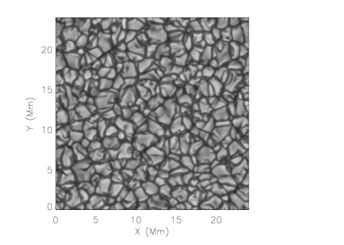
The MURaM code (Vögler 2003, Vögler et al. 2005) treats the equations of compressible (magneto-) hydrodynamics, incorporating radiative transfer and partial ionization effects in local thermal equilibrium. The simulation run analysed here has a domain size of $24\times 24\times 2.3$ $\mathrm{Mm}^{3}$, with periodic horizontal boundary conditions. The $\tau=1$ level is located roughly $600$ km below the top of the simulation box. The grid resolution is $20.8$ km in the horizontal and $14$ km in vertical direction. The magnetic field is set to zero. The bottom boundary is open and allows for mass flow. The top boundary is closed, with vanishing horizontal viscous stress. The total length of the simulation run is $11$ hours. Figure 1 shows a brightness snapshot from the simulation.

Figure 1: Bolometric brightness distribution from the simulation. Plasma flows upward in the bright cell interiors (granules) and back into the interior in the darker intergranular lanes.

Figure 2: Top left: LCT horizontal velocity divergence field (grey-scale, bright: positive, dark: negative) and the velocity arrows, temporally averaged over $60$ minutes. The longest arrows correspond to velocities of $\sim 540$ $\mathrm{ms^{-}1}$. Top right : the same LCT horizontal velocity divergence field, overplotted with the contours of the corresponding divergence of the actual flow velocity averaged spatially over the LCT window size. Solid lines indicate positive divergence, dashed negative divergence. Bottom left: corresponding velocity divergence patches (mesogranules) lying above the $0.5\Lambda$ threshold (see explanation in Sect. 4). Bottom right: the same but for the $0.7\Lambda$ threshold.

3 Local Correlation Tracking

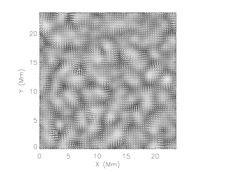
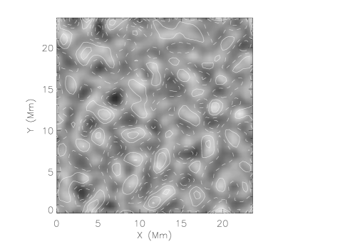
In observations and simulations mesogranules are often identified with areas of positive horizontal velocity divergence (Roudier et al. 1998, Cattaneo et al. 2001, Leitzinger et al. 2005). In observations the horizontal velocity field is obtained with a LCT algorithm, which tracks intensity patterns on the surface. Figure 2 (top left panel) shows the divergence of horizontal velocity obtained from the simulation with the LCT method, averaged over $60$ min, along with the corresponding velocity arrows. We use the LCT algorithm described by Welsh et al. (2004), with the tracking window being a Gaussian with FWHM of $1$ Mm. Using data from the MURaM simulation, we find that the LCT velocities are roughly between $0.5-0.7$ in magnitude as compared to the actual plasma velocities around continuum optical depth unity (see also Rieutord et al. 2001, Georgobiani et al. 2007). The top right panel of Fig. 2 shows the LCT velocity divergence field overplotted with contours of the divergence of the actual velocity from the simulation, averaged spatially over the LCT window size. Both velocity fields are temporally averaged over $60$ minutes and have a cross correlation coefficient $0.75$. The mean correlation value between the divergences of the LCT and actual plasma velocities for the whole dataset equals $0.73$.

Figure 3: Top: correlation between the LCT velocities and the horizontal plasma velocities coming from different depths of the simulation box. Bottom: Correlation between the LCT velocity divergence and vertical plasma velocities coming from different depths of the simulation box. The solid line represents the correlation coefficient as a function of depth for the $47$-min average of the data. The dashed line shows the correlation coefficients calculated individually for each of the $81$ velocity snapshots within the $47$ minutes, and then averaged.

Figure 4: Mesogranule lifetime (top) and size histograms (middle), together with a scatter plot of area versus lifetime (bottom). The threshold level and averaging time are $0.5\Lambda$ and $t_{a}=60$ min., respectively. Dotted lines represent power-law fits with exponents $-1.2$ for the lifetime and $-2.4$ for the area, respectively.

Considering horizontal velocity vector fields, we investigate the correlation between the LCT velocities and the plasma velocities coming from different heights of the simulation box. Upper panel of Fig. 3 shows the correlation coefficient as a function of depth. The zero height level is chosen at the spatial average of the level of optical depth unity. The actual plasma velocities have been spatially averaged over the LCT tracking window size. The solid line corresponds to a correlation coefficient of a $47$-minute average of both velocity fields, while the dotted-dashed line shows an average of the correlation coefficients calculated individually for each of the $81$ velocity snapshots within the $47$ minutes. Clearly, time-averaging increases the correlation between the two velocity fields, indicating that the LCT velocities are a reliable representation of the plasma velocities, in particular at timescales longer than granule lifetime scale. We find the highest correlation coefficients for the plasma velocities coming from roughly $100$ km below the surface. Similar results were found by Rieutord et al. (2001) using a simulation with a much coarser horizontal resolution of $95$ km.

The correlation decreases rapidly with depth in the top panel of Figure 3. This does not, however, indicate that the LCT velocities do not reflect deeper convective structures. To investigate this we look at the correlation between the LCT velocity divergence and the actual vertical plasma velocities as a function of depth. The results are shown in the bottom panel of Figure 3. The vertical velocities here were spatially smoothed using a filter of the same size as the LCT tracking window. These results indicate that the LCT algorithm is detecting the organization of convective structures which extend at least as deep as the simulation (ie to deeper than $-1.7$ Mm below the surface). While the horizontal velocities show less organization in the deeper layers (they are mainly resulting from mass conservation in the strongly stratified system), the vertical velocities are strongly affected by the pattern of downflows, which stays roughly the same from the surface to the bottom of the simulation box.

4 Mesogranular flow patterns

4.1 Definition

We define mesogranules in the simulation as patches of positive horizontal velocity divergence, analogous to the definition used in the case of solar observations and also in the two-dimensional cellular model of Matloch et al. (2009). The analysis procedure is identical for both the cellular model and the numerical simulation. The intensity images from the simulation have a cadence of $30$ sec. The first step is to apply the LCT algorithm to extract the horizontal velocity field from the displacement of granules. Then we average the resulting velocity fields over a given averaging time, $t_{a}$, and calculate the velocity divergence. Next, mesogranules are identified as patches for which the divergence exceeds a predefined threshold value. The level is set in the following way: for each $t_{a}$-averaged map, the rms value of the velocity divergence is determined, and then the time average of the rms, $\Lambda$, over the whole dataset is calculated. In addition, all patches smaller than $0.7$ of the average granule area are disregarded, to be consistent with the two-dimensional cellular model.

Individual mesogranules are tracked in time and both their lifetime and the lifetime-averaged area are determined. The tracking algorithm works as follows: first, the mesogranules are labelled in each mesogranule image. Next, for each pair of subsequent mesogranule images, the algorithm finds the mesogranules that show the maximum overlap in both images. Unless a splitting has occurred, such cells are taken to be the same mesogranule. The above scheme works well because the cadence of the divergence images is sufficiently high ($30$ sec) so that the mesogranules do not significantly shift their position between subsequent images. The panels at the bottom of Fig. 2 show an example of the velocity divergence patches (mesogranules) lying above the $0.5\Lambda$ threshold (left panel), and $0.7\Lambda$ threshold (right panel) for the averaging time $t_{a}=60$ min.

Figure 5: Dependence of the mean mesogranule lifetime on the averaging time (top) and of mean mesogranule area on the spatial smoothing window size (bottom).

4.2 Properties

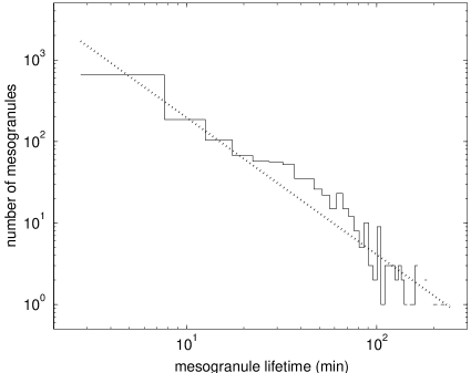
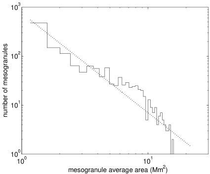
Figure 4 shows the mesogranule statistics obtained for a threshold level of $0.5\Lambda$ and an averaging time $t_{a}=60$ min. Both histograms are well approximated by power laws, with exponents $-1.2$ for lifetime and $-2.4$ for the area, similar to the result obtained from the two-dimensional cellular model, where exponents $-1.3$ and $-3.4$ were found, respectively. (see Fig. 17 in Matloch et al. 2009). The power-law behaviour of the distributions suggests that no characteristic scales are associated with the pattern.

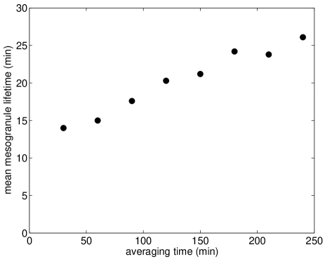
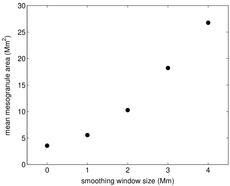
We investigate how the mean mesogranule properties depend on the analysis parameters: the averaging time $t_{a}$, the spatial smoothing window size and the divergence threshold level. The LCT procedure introduces spatial smoothing due to the LCT tracking window, which has to be of the size of the tracers (here granules). Hence, the flow field obtained by LCT is effectively filtered from all contributions below a spatial scale of roughly $2.5$ Mm (Rieutord et al. 2001, 2010). We take the actual plasma velocities, and apply spatial smoothing windows of different sizes, as well as different averaging times, in order to study how it influences the resulting mesogranular pattern. Figure 5 shows the dependence of the mean mesogranule lifetime on the averaging time, $t_{a}$ (upper panel), and the dependence of the mean mesogranule area on the smoothing window size (lower panel). The lifetime increases roughly linearly with the averaging time, while the area increases as a square of the spatial smoothing window size. We also find that the mean mesogranule area does not depend on the averaging time. These results are similar to those from the cellular model (see Fig. 18 in Matloch et al. 2009), and imply that the mesogranular pattern has no characteristic scale.

So far we have seen that the velocity divergence field and the corresponding mesogranular pattern produced in the numerical simulation are similar to that resulting from the cellular model (Matloch et al. 2009). To further investigate the structure of the divergence fields in both models, we plot in Fig. 6 the dependence of the average mesogranule size (obtained for a fixed averaging time $t_{a}=1$ hour) on the threshold value, $\Lambda$, for mesogranule definition. The values of the mesogranule area have been normalized so that the area equals $1$ for a threshold of $0.1\Lambda$ for both models.

Figure 6: Dependance of the mean mesogranule area on the threshold value for the cellular model (solid line) and the numerical simulation (dashed-dotted line), obtained for an averaging time of $60$ min. The values of the mesogranule area have been normalized so that the area equals $1$ for a threshold of $0.1\Lambda$ for both models.

The behaviour of the curves in Fig. 6 is similar: they can be approximated with a power law with exponents $-1.5$ and $-1.1$ for the cellular model and numerical simulation, respectively. This supports the conclusion that the structure of the velocity divergence field on scales larger than granulation produced by the cellular model is very similar to that in the MURaM simulation.

5 Conclusions

We found mesogranular structures in a shallow (bottom $\sim 1.7$ Mm below $\tau=1$ level) hydrodynamical simulation of solar surface convection. The mesogranules were found to have no intrinsic temporal or spatial scales and showed a power-law distribution of sizes and lifetimes. The mean values depended on the averaging times and the size of the spatial smoothing window used in the analysis. The LCT velocity was found to be correlated with real convective motions: horizontal velocities near the surface and vertical velocities across a broad height range.

The properties of mesogranular flow patterns emerging in the numerical simulation correspond very well to those in the cellular model (Matloch et al. 2009) when the same analysis methods are used in both models. The distributions of mesogranule areas and lifetimes, as well as the dependence of the mean values of the mesogranule area and lifetime on the analysis parameters, follow the same laws. This suggests that the mesogranular flows do not represent a distinct convective scale.

References

- Cardena et al. (2003) Domínguez Cardeña, I. 2003, A&A, 412, L65
- Cattaneo et al. (2001) Cattaneo, F., Lenz, D., & Weiss, N. 2001, ApJ, 563, L91
- Georgobiani et al. (2007) Georgobiani, D., Zhao, J., Kosovichev, A. G., Benson, D., Stein, R. F., & Nordlund, Å. 2007, ApJ, 657, 1157
- Leitzinger et al. (2005) Leitzinger, M., Brandt, P. N., Hanslmeier, A., Pötzi, W., & Hirzberger, J. 2005, A&A, 444, 245
- Matloch et al. (2009) Matloch, L., Cameron, R.,Schmitt, D., & Schüssler, M. 2009, A&A, 504, 1041M
- Nordlund (2005) Nordlund, . 1985, Solar Phys., 100, 209
- Nordlund et al. (2009) Nordlund, , Stein, R. F., & Asplund, M. 2009, Liv. Rev. in Sol. Phys., 6, 2
- November et al. (1981) November, L. J., Toomre, J., Gebbie, K. B., & Simon, G. W. 1981, ApJ, 245, L123
- Ploner et al. (1999) Ploner, S. R. O., Solanki, S. K., & Gadun, A. S. 1999, A&A, 352, 679
- Ploner et al. (2000) Ploner, S. R. O., Solanki, S. K., & Gadun, A. S. 2000, A&A, 356, 1050
- Rieutord et al. (2001) Rieutord, M., Roudier, T., Ludwig, H.-G., Nordlund, Å., & Stein, R. 2001, A&A, 377, L14
- Rieutord et al. (2010) Rieutord, M., Roudier, T., Rincon, F., Malherbe, J. M., Meunier, N., Berger, T., Frank, Z., 2010, A&A, 512A, 4R
- Roudier et al. (1998) Roudier, Th., Malherbe, J. M., Vigneau, J., & Pfeiffer, B. 1998, A&A, 330, 1136
- Roudier et al. (2003) Roudier, Th., Lignières, F., Rieutord, M., Brandt, P. N., & Malherbe, J. M. 2003, A&A, 409, 299
- Simon et al. (1991) Simon, G. W., Title, A. M., & Weiss, N. O. 1991, ApJ, 375, 775
- Stein et al. (1998) Stein , R. F., & Nordlund, Å. 1998, ApJ, 499, 914
- Vögler (2003) Vögler, A., 2003, PhD Thesis, Univ. Göttingen, http://webdoc.sub.gwdg,de/diss/2004/voegler/
- Vögler et al. (2005) Vögler, A., Shelyag, S., Schüssler, M., Cattaneo, F., Emonet, T., & Linde,T. 2005, A&A, 429, 335
- Welsh et al. (2004) Welsh, B. T., Fisher, G. H., & Abbett, W. P., 2004, ApJ, 610, 1148